Posts Tagged Machine Learning
Unlocking the Potential of Generative AI for Synthetic Data Generation
Posted by Gary A. Stafford in AI/ML, Cloud, Enterprise Software Development, Machine Learning, Python, Software Development, Technology Consulting on April 18, 2023
Explore the capabilities and applications of generative AI to create realistic synthetic data for software development, analytics, and machine learning

Introduction
Generative AI refers to a class of artificial intelligence algorithms capable of generating new data similar to a given dataset. These algorithms learn the underlying patterns and relationships in the data and use this knowledge to create new data consistent with the original dataset. Generative AI is a rapidly evolving field that has the potential to revolutionize the way we generate and use data.
Generative AI can generate synthetic data based on patterns and relationships learned from actual data. This ability to generate synthetic data has numerous applications, from creating realistic virtual environments for training and simulation to generating new data for machine learning models. In this article, we will explore the capabilities of generative AI and its potential to generate synthetic data, both directly and indirectly, for software development, data analytics, and machine learning.
Common Forms of Synthetic Data
According to AltexSoft, in their article Synthetic Data for Machine Learning: its Nature, Types, and Ways of Generation, common forms of synthetic data include:
- Tabular data: This type of synthetic data is often used to generate datasets that resemble real-world data in terms of structure and statistical properties.
- Time series data: This type of synthetic data generates datasets that resemble real-world time series data. It is commonly used when real-world time series data is unavailable or too expensive.
- Image and video data: This synthetic data is used to generate realistic images and videos for training machine learning models or simulations.
- Text data: This synthetic data generates realistic text for natural language processing tasks or for generating training data for machine learning models.
- Sound data: This synthetic data generates realistic sound for training machine learning models or simulations.
Synthetic Tabular Data Types
Synthetic tabular data refers to artificially generated datasets that resemble real-world tabular data in terms of structure and statistical properties. Tabular data is organized into rows and columns, like tables or spreadsheets. Some specific types of synthetic tabular data include:
- Financial data: Synthetic datasets that resemble real-world financial data such as bank transactions, stock prices, or credit card information.
- Customer data: Synthetic datasets that resemble real-world customer data, such as purchase history, demographic information, or customer behavior.
- Medical data: Synthetic datasets that resemble real-world medical data, such as patient records, medical test results, or treatment history.
- Sensor data: Synthetic datasets that resemble real-world sensor data such as temperature readings, humidity levels, or air quality measurements.
- Sales data: Synthetic datasets that resemble real-world sales data, such as sales transactions, product information, or customer behavior.
- Inventory data: Synthetic datasets that resemble real-world inventory data, such as stock levels, product information, or supplier information.
- Marketing data: Synthetic datasets that resemble real-world marketing data, such as campaign performance, customer behavior, or market trends.
- Human resources data: Synthetic datasets that resemble real-world human resources data, such as employee records, performance evaluations, or salary information.
Challenges with Creating Synthetic Data
According to sources including Towards Data Science, enov8, and J.P. Morgan, there are several challenges in creating synthetic data, including:
- Technical difficulty: Properly modeling complex real-world behaviors such as synthetic data is challenging, given available technologies.
- Biased behavior: The flexible nature of synthetic data makes it prone to potentially biased results.
- Privacy concerns: Care must be taken to ensure synthetic data does not reveal sensitive information.
- Quality of the data model: If the quality of the data model is not high, wrong conclusions can be reached.
- Time and effort: Synthetic data generation requires time and effort.
Difficult Patterns and Behaviors to Model
Many patterns and behaviors can be challenging to model in synthetic data, for example:
- Rare events: If certain events rarely occur in the real world, generating synthetic data that accurately reflects their distribution can be difficult.
- Complex relationships: Synthetic data generators may struggle to capture complex relationships between variables, such as non-linear interactions, feedback loops, or conditional dependencies.
- Contextual variability: Contextual factors, such as time, location, or individual differences, can have a significant impact on the distribution of data. Modeling this variability accurately can be challenging.
- Outliers and anomalies: Synthetic data generators may be unable to generate outliers or anomalies that are realistic and representative of the real world.
- Dynamic data: If the data is dynamic and changes over time, it can be challenging to generate synthetic data that captures these changes accurately.
- Unobserved variables: Sometimes, variables may be necessary for understanding the data distribution but are not directly observable. These variables can be challenging to model in synthetic data.
- Data bias: If the real-world data is biased in some way, such as over-representation of certain groups or under-representation of others, it can be challenging to generate synthetic data that is unbiased and representative of the population.
- Time-dependent patterns: If the data exhibits time-dependent patterns, such as seasonality or trends, it can be challenging to generate synthetic data that accurately reflects them.
- Spatial patterns: If the data has a spatial component, such as location data or images, it can be challenging to generate synthetic data that captures the spatial patterns realistically.
- Data sparsity: If the data is sparse or incomplete, it can be difficult to generate synthetic data that accurately reflects the distribution of the entire dataset.
- Human behavior: If the data involves human behavior, such as in social science or behavioral economics, it can be challenging to model the complex and nuanced behaviors of individuals and groups.
- Sensitive or confidential information: In some cases, the data may contain sensitive or confidential information that cannot be shared, making it challenging to generate synthetic data that preserves privacy while accurately reflecting the underlying distribution.
Overall, many patterns can be challenging to model accurately in synthetic data. It often requires careful consideration of the specific data characteristics and the synthetic data generation techniques’ limitations.
Easily Modeled Patterns and Behaviors
There are many simple and well-understood patterns that can be easily modeled in synthetic data, for example:
- Randomness: If the data is purely random, it can be easily generated using a random number generator or other simple techniques.
- Gaussian distribution: If the data follows a Gaussian or normal distribution, it can be generated using a Gaussian random number generator.
- Uniform distribution: If the data follows a uniform distribution, it can be easily generated using a uniform random number generator.
- Linear relationships: If the data follows a linear relationship between variables, it can be modeled using simple linear regression techniques.
- Categorical variables: If the data consists of categorical variables, such as gender or occupation, it can be generated using a categorical distribution.
- Text data: If the data consists of text, it can be generated using natural language processing techniques, such as language models or text generation algorithms.
- Time series: If the data consists of time series data, such as stock prices or weather data, it can be generated using time series models, such as Autoregressive integrated moving average (ARIMA) or Long short-term memory (LSTM).
- Seasonality: If the data exhibits seasonal patterns, such as higher sales data during holiday periods, it can be generated using seasonal time series models.
- Proportions and percentages: If the data consists of proportions or percentages, such as product sales distribution across different regions, it can be generated using beta or Dirichlet distributions.
- Multivariate normal distribution: If the data follows a multivariate normal distribution, it can be generated using a multivariate Gaussian random number generator.
- Networks: If the data consists of network or graph data, such as social networks or transportation networks, it can be generated using network models, such as Erdos-Renyi or Barabasi-Albert models.
- Binary data: If the data consists of binary data, such as whether a customer churned, it can be generated using a Bernoulli distribution.
- Geospatial data: If it involves geospatial data, such as the location of points of interest, it can be easily using geospatial models, such as point processes or spatial point patterns.
- Customer behaviors: If the data involves customer behaviors, such as browsing or purchase histories, it can be generated using customer journey models, such as Markov models.
In general, simple and well-understood patterns can be easily modeled using synthetic data techniques. In contrast, more complex and nuanced patterns may require more sophisticated modeling techniques and a deeper understanding of the underlying data characteristics.
Creating Synthetic Data with Generative AI
We can use many popular generative AI-powered tools to create synthetic data for testing applications, constructing analytics pipelines, and building machine learning models. Tools include OpenAI ChatGPT, Microsoft’s all-new Bing Chat, ChatSonic, Tabnine, GitHub Copilot, and Amazon CodeWhisperer. For more information on these tools, check out my recent blog post:
Accelerating Development with Generative AI-Powered Coding Tools
Explore six popular generative AI-powered tools, including ChatGPT, Copilot, CodeWhisperer, Tabnine, Bing, and…garystafford.medium.com
Let’s start with a simple example of generating synthetic sales data. Suppose we have created a new sales forecasting application for coffee shops that we need to test using synthetic data. We might start by prompting a generative AI tool like OpenAI’s ChatGPT for some data:
Create a CSV file with 25 random sales records for a coffee shop.
Each record should include the following fields:
  - id (incrementing integer starting at 1)
  - date (random date between 1/1/2022 and 12/31/2022)
  - time (random time between 6:00am and 9:00pm in 1-minute increments)
  - product_id (incrementing integer starting at 1)
  - product
  - calories
  - price in USD
  - type (drink or food)
  - quantity (random integer between 1 and 3)
  - amount (price * quantity)
  - payment type (cash, credit, debit, or gift card)
The content and structure of a prompt can vary, and this can strongly influence ChatGPT’s response. Based on the above prompt, the results were accurate but not very useful for testing our application in this format. ChatGPT cannot create a physical CSV file. Furthermore, ChatGPT’s response length is limited; only about twenty records were returned. According to ChatGPT, in general, ChatGPT can generate responses of up to 2,048 tokens, the maximum output length allowed by the GPT-3 model.

Instead of outputting the actual synthetic data, we could ask ChatGPT to write a program that can, in turn, generate the synthetic data. This option is certainly more scalable. Let’s prompt ChatGPT to write a Python program to generate synthetic sales data with the same characteristics as before:
Create a Python3 program to generate 100 sales of common items
sold in a coffee shop. The data should be written to a CSV file
and include a header row. Each record should include the following fields:
  - id (incrementing integer starting at 1)
  - date (random date between 1/1/2022 and 12/31/2022)
  - time (random time between 6:00am and 9:00pm in 1-minute increments)
  - product_id (incrementing integer starting at 1)
  - product
  - calories
  - price in USD
  - type (drink or food)
  - quantity (random integer between 1 and 3)
  - amount (price * quantity)
  - payment type (cash, credit, debit, or gift card)
Using a single concise prompt, ChatGPT generated a complete Python program, including code comments, to generate synthetic sales data. Unfortunately, given ChatGPT’s response size limitation, the coffee shop menu was limited to just six items. Reprompting for more items would result in the truncation of the output and, thus, the program, making it unrunnable. Instead, we could use an additional prompt to generate a longer Python list of menu items and combine the two pieces of code in our IDE. Regardless, we will still need to copy and paste the code into our IDE to review, debug, test, and run.

ChatGPT’s Python program, copied and pasted into VS Code, ran without modifications, and wrote 100 synthetic sales records to a CSV file!

Using IDE-based Generative AI Tools
Although generating synthetic data directly or snippets of code in chat-based generative AI tools are helpful for limited use cases, writing code in IDE gives us several advantages:
- Code does not need to be copied and pasted from external sources into an IDE
- Consecutive lines of code, method, and block code completion overcome the single response size limits of chat-based tools like OpenAI ChatGPT
- Code can be reused and adapted to evolving use cases over time
- Python interpreter and debugger or equivalent for other languages
- Automatic code formatting, linting, and code style enforcement
- Unit, integration, and functional testing
- Static code analysis (SCA)
- Vulnerability scanning
- IntelliSense for code completion
- Source code management (SCM) / version control
Let’s use the same techniques we used with ChatGPT, but from within an IDE to generate three types of synthetic data. We will choose Microsoft’s VS Code with GitHub Copilot and Python as our programming language.

Source Code
All the code examples shown in this post can be found on GitHub.
Example #1: Coffee Shop Sales Data
First, we will start by outlining the program’s objective using code comments on the top of our Python file. This detailed context helps us to clearly express our goal and enables Copilot to generate an accurate response.
# Write a program that creates synthetic sales data for a coffee shop.
# The program should accept a command line argument that specifies the number of records to generate.
# The program should write the sales data to a file called 'coffee_shop_sales_data.csv'.
# The program should contain the following functions:
#   - main() function that calls the other functions
#   - function that returns one random product from a list of dictionaries
#   - function that returns a dictionary containing one sales record
#   - function that writes the sales records to a file
Following the import statements also generated with the assistance of Copilot, we will write the first function to return a random product from a list of 25 products. Again, we will use code comments as a prompt to generate the code. Copilot was able to generate 100% of the function’s code from the comments.
# Write a function to create list of dictionaries.
# The list of dictionaries should contain 15 drink items and 10 food items sold in a coffee shop.
# Include the product id, product name, calories, price, and type (Food or Drink).
# Capilize the first letter of each product name.
# Return a random item from the list of dictionaries.
Below is an example of Copilot’s ability to generate complete lines of code. Ultimately, it generated 100% of the function including choosing the items sold in a coffee shop, with a reasonable price and caloric count. Copilot is not limited to just understanding code.

Next, we will write a function to return a random sales record.
# Write a function to return a random sales record.
# The record should be a dictionary with the following fields:
#   - id (an incrementing integer starting at 1)
#   - date (a random date between 1/1/2022 and 12/31/2022)
#   - time (a random time between 6:00am and 9:00pm in 1 minute increments)
#   - product_id, product, calories, price, and type (from the get_product function)
#   - quantity (a random integer between 1 and 3)
#   - amount (price * quantity)
#   - payment type (Cash, Credit, Debit, Gift Card, Apple Pay, Google Pay, or Venmo)
Again, Copilot generated 100% of the function’s code as a single block based on the code comments.

Lastly, we will create a function to write the sales data into a CSV file using Copilot’s help.
# Write a function to write the sales records to a CSV file called 'coffee_shop_sales.csv'.
# Use an input parameter to specify the number of records to write.
# The CSV file must have a header row and be comma delimited.
# All string values must be enclosed in double quotes.
Again below, we see an example of Copilot’s ability to generate an entire Python function. I needed to correct a few problems with the generated code. First, there was a lack of quotes for string values, which I added to the function (quotechar='"', quoting=csv.QUOTE_NONNUMERIC). Also, the function was missing a key line of code, sale = get_sales_record(), which would have caused the code to fail. Remember, just because the code was generated does not mean it is correct.

Here is the complete program that creates synthetic sales data for a coffee shop with Copilot assistance:
Copilot generated an astounding 80–85% of the program’s final code. The initial program took 10–15 minutes to write using code comments. I then added a few new features, including the ability to pass in the record count on the command line and the hash-based transaction id, which took another 5 minutes. Finally, I used GitHub Code Brushes to optimize the code and generate the Python docstrings, and Black Formatter and Flake8 extensions to format and lint, all of which took less than 5 minutes. With testing and debugging, the total time was about 25–30 minutes.
The most significant difference with Copilot was that I never had to leave the IDE to look up code references or find existing sales datasets or even a coffee shop menu to duplicate. The code, as well as the list of products, price, calories, and product type, were all generated by Copilot.
To make this example more realistic, you could use Copilot’s assistance to write algorithms capable of reflecting daily, weekly, and seasonal variations in product choice and sales volumes. This might include simulating increased sales during the busy morning rush hour or a preference for iced drinks in the summer months versus hot drinks during the winter months.
Here is an example of the synthetic sales data output by the example application:
Example #2: Residential Address Data
We could use these same techniques to generate a list of residential addresses. To start, we can prompt Copilot for the values in a list of common street names and street types in the United States:
# Write a function that creates a list of common street names
# in the United States, in alphabetical order.
# List should be in alphabetical order. Each name should be unique.
# Return a random street name.
def get_street_name():
    street_names = [
        "Ash", "Bend", "Bluff", "Branch", "Bridge", "Broadway", "Brook", "Burg",
        "Bury", "Canyon", "Cape", "Cedar", "Cove", "Creek", "Crest", "Crossing",
        "Dale", "Dam", "Divide", "Downs", "Elm", "Estates", "Falls", "Fifth",
        "First", "Fork", "Fourth", "Glen", "Green", "Grove", "Harbor", "Heights",
        "Hickory", "Hill", "Hollow", "Island", "Isle", "Knoll", "Lake", "Landing",
        ...
    ]

    return random.choice(street_names)


# Write a function that creates a list of common street types
# in the United States, in alphabetical order.
# List should be in alphabetical order. Each name should be unique.
# Return a random street type.
def get_street_type():
    street_types = [
        "Alley", "Avenue", "Bend", "Bluff", "Boulevard", "Branch", "Bridge", "Brook",
        "Burg", "Circle", "Commons", "Court", "Drive", "Highway", "Lane", "Parkway",
        "Place", "Road", "Square", "Street", "Terrace", "Trail", "Way"
    ]

    return random.choice(street_types)
Next, we can create a function that returns a property type based on a categorical distribution of common residential property types with the prompt:
# Write a function to return a random property type.
# Accept a random value between 0 and 1 as an input parameter.
# The function must return one of the following values based on the %:
# 63% Single-family, 26% Multi-family, 4% Condo,
# 3% Townhouse, 2% Mobile home, 1% Farm, 1% Other.
Again, Copilot generated 100% of the function’s code as a single block based on the code comments.

Additionally, we could have Copilot help us generate a list of the 50 largest cities in the United States with state, zip code, and population, with the prompt:
# Write a function to returns the 50 largest cities in the United States.
# List should be sorted in descending order by population.
# Include the city, state abbreviation, zip code, and population.
# Return a list of dictionaries.
Once again, Copilot generated 100% of the function’s code using a combination of single lines and code blocks based on the code comments.

When randomly choosing a city, we can use a categorical distribution of populations of all the cities to control the distribution of cities in the final synthetic dataset. For example, there will be more addresses in larger cities like New York City or Los Angeles than in smaller cities like Buffalo or Virginia Beach, with the prompt:
# Write a function that calculates the total population of the list of cities.
# Add a 'pcnt_of_total_population' and 'pcnt_running_total' columns to list.
# Returns a sorted list of cities by population.
Here is the complete program that creates synthetic US-based address data with Copilot assistance:
To make this example more realistic, you could use Copilot’s assistance to write algorithms capable of accurately reflecting assessed property values based on the type of residence and the zip code.
Here is an example of the synthetic US-based residential address data output by the example application:
Example #3: Demographic Data
We could use the same techniques again to generate synthetic demographic data. With the assistance of Copilot, we can write functions that randomly return typical feminine or masculine first names (forenames) and common last names (surnames) found in the United States, for this use case.
# Write a function that generates a list of common feminine first names in the United States.
# List should be in alphabetical order.
# Each name should be unique.
# Return random first name.
def get_first_name_feminine():
    first_name_feminine = [
        "Alice", "Amanda", "Amy", "Angela", "Ann", "Anna", "Barbara", "Betty",
        "Brenda", "Carol", "Carolyn", "Catherine", "Christine", "Cynthia", "Deborah", "Debra",
        "Diane", "Donna", "Doris", "Dorothy", "Elizabeth", "Frances", "Gloria", "Heather",
        "Helen", "Janet", "Jennifer", "Jessica", "Joyce", "Julie", "Karen", "Kathleen", "Kimberly",
    ]

    return random.choice(first_name_feminine)
With the assistance of Copilot, we can also write functions that return demographic information, such as age, gender, race, marital status, religion, and political affiliation. Similar to the previous sales data example, we can influence the final synthetic dataset based on categorical distributions of different demographic categories, for instance, with the prompt:
# Write a function that returns a person's martial status.
# Accept a random value between 0 and 1 as an input parameter.
# The function must return one of the following values based on the %:
# 50% Married, 33% Single, 17% Unknown.
def get_martial_status(rnd_value):
    if rnd_value < 0.50:
        return "Married"
    elif rnd_value < 0.83:
        return "Single"
    else:
        return "Unknown"
By altering the categorical distributions, we can quickly alter the resulting synthetic dataset to reflect differing demographic characteristics: an older or younger population, the predominance of a single race, religious affiliation, or marital status, or the ratio of males to females.
Next, we can use a Gaussian distribution (aka normal distribution) to return the year of birth in a bell-shaped curve, given a mean year and a standard deviation, using Python’s random.normalvariate function.
# Write a function that generates a normal distribution of date of births.
# with a mean year of 1975 and a standard deviation of 10.
# Return random date of birth as a string in the format YYYY-MM-DD
def get_dob():
    day_of_year = random.randint(1, 365)
    year_of_birth = int(random.normalvariate(1975, 10))
    dob = date(int(year_of_birth), 1, 1) + timedelta(day_of_year - 1)
    dob = dob.strftime("%Y-%m-%d")
    return dob
Here is the complete program that creates synthetic demographic data with Copilot’s assistance:
To make this example more realistic, you could use Copilot’s assistance to write algorithms capable of more accurately representing the nuanced associations and correlations between age, gender, race, marital status, religion, and political affiliation.
Here is an example of the synthetic demographic data output by the example application:
Generative AI Tools for Unit Testing
In addition to writing code and documentation, a common use of generative AI code assistants like Copilot is unit tests. For example, we can create unit tests for each function in our coffee shop sales data code generator, using the same method of prompting with code comments.

Conclusion
In this post, we learned how Generative AI could assist us in creating synthetic data for software development, analytics, and machine learning. The examples herein generated data using simple techniques. Using advanced modeling techniques, we could generate increasingly complex, realistic synthetic data.
To learn about other ways Generative AI can be used to assist in writing code, please read my previous article, Ten Ways to Leverage Generative AI for Development on AWS.
🔔 To keep up with future content, follow Gary Stafford on LinkedIn.
This blog represents my viewpoints and not those of my employer, Amazon Web Services (AWS). All product names, logos, and brands are the property of their respective owners.
Navigating the World of Generative AI: A Guide to Essential Terminology
Posted by Gary A. Stafford in AI/ML, Machine Learning, Technology Consulting on April 9, 2023
Learn the essential terms and concepts you need to know to navigate the rapidly evolving world of generative AI

Generative AI is a fascinating and rapidly evolving field that has the potential to transform the way we interact with technology. However, with so much buzz and hype surrounding this topic, making sense of it all can be challenging. In this article, we’ll cut through the noise and gain a clear understanding of the essential terminology you need to know to navigate the world of generative AI.
According to a variety of sources, including McKinsey & Company and Vox Media, the critical difference between generative AI and other emerging technologies is that millions of people can — and already are — using it to create new content, such as text, photos, video, code, and 3D renderings, from data it is trained on. Recent breakthroughs in the field have the potential to drastically change the way we approach content creation. This has led to widespread excitement and some understandable apprehension about the potential for generative AI to impact virtually every aspect of society and disrupt industries, including media and entertainment, healthcare and life sciences, education, advertising, legal services, and finance.
Even if your current role is not in technology, it is highly likely that generative AI will have a direct impact on both your personal and professional life.
Gary Stafford
Even if your current role is not in technology, it is highly likely that generative AI will have a direct impact on both your personal and professional life. Familiarizing yourself with basic terminology related to generative AI can help you better comprehend the discussions on social media and in the news.
Terminology
Let’s explore the following terminology (in alphabetical order):
- Artificial General Intelligence (AGI)
- Artificial Intelligence (AI)
- ChatGPT
- DALL·E
- Deep Learning (DL)
- Generative AI
- Generative Pre-trained Transformer (GPT)
- Intelligence Amplification (IA)
- Large Language Model (LLM)
- Machine Learning (ML)
- Neural Network
- OpenAI
- Prompt Engineering
- Reinforcement Learning with Human Feedback (RLHF).
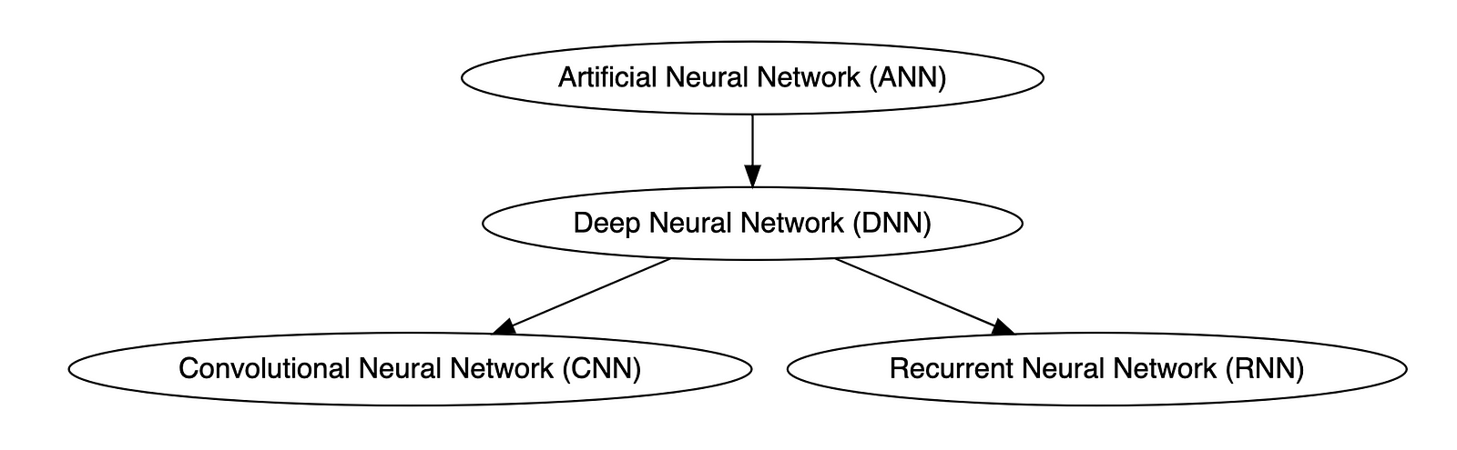
Below is a knowledge graph, created with OpenAI ChatGPT, showing the approximate relationships between the post’s terms.

Artificial General Intelligence (AGI)
According to the all-new Bing Chat, based on ChatGPT, artificial general intelligence (AGI) is the ability of an intelligent agent to understand or learn any intellectual task that human beings or other animals can. It is a primary goal of some artificial intelligence research and a common topic in science fiction and Futurism. According to Forbes, which also prompted ChatGPT, Artificial General Intelligence (AGI) refers to a theoretical type of artificial intelligence that possesses human-like cognitive abilities, such as the ability to learn, reason, solve problems, and communicate in natural language.
Eliezer Yudkowsky is an American researcher, writer, and philosopher on the topic of AI. The podcast Eliezer Yudkowsky: Dangers of AI and the End of Human Civilization, by prominent MIT Research Scientist Lex Fridman, explores various aspects of artificial general intelligence against the backdrop of the recent release of OpenAI’s GPT-4.
Artificial Intelligence (AI)
According to the Brookings Institute, AI is generally thought to refer to machines that respond to stimulation consistent with traditional responses from humans, given the human capacity for contemplation, judgment, and intention. Similarly, according to the U.S. Department of State, the term artificial intelligence refers to a machine-based system that can, for a given set of human-defined objectives, make predictions, recommendations, or decisions influencing real or virtual environments.

ChatGPT
ChatGPT, according to ChatGPT, is a large language model developed by OpenAI. I was trained on a massive dataset of human-written text using a deep neural network (DNN) architecture called GPT (Generative Pre-trained Transformer). Its purpose is to generate human-like responses to questions and prompts, engage in conversations, and perform various language-related tasks. It is a virtual assistant capable of understanding and generating natural language.
DALL·E
According to Wikipedia, DALL·E is a deep learning model developed by OpenAI to generate digital images from natural language descriptions, called prompts. DALL·E is a portmanteau of the names of the animated robot Pixar character WALL-E and the Spanish surrealist artist Salvador Dalí. According to OpenAI, DALL·E is an AI system that can create realistic images and art from a description in natural language. OpenAI introduced DALL·E in January 2021. One year later, in April 2022, they announced their newest system, DALL·E 2, which generates more realistic and accurate images with 4x greater resolution. DALL·E 2 can create original, realistic images and art from a text description. It can combine concepts, attributes, and styles.
Deep Learning (DL)
According to IBM, deep learning is a subset of machine learning (ML), which is essentially a neural network with three or more layers. These neural networks attempt to simulate the behavior of the human brain — albeit far from matching its ability — allowing it to “learn” from large amounts of data. While a neural network with a single layer can still make approximate predictions, additional hidden layers can help to optimize and refine for accuracy.
Generative AI
According to Wikipedia, generative artificial intelligence (AI), aka generative AI, is a type of AI system capable of generating text, images, or other media in response to prompts. Generative AI systems use generative models such as large language models (LLMs) to statistically sample new data based on the training data set used to create them.
Generative Pre-trained Transformer (GPT)
According to ChatGPT, Generative Pre-trained Transformer (GPT) is a deep learning architecture used for natural language processing (NLP) tasks, such as text generation, summarization, and question-answering. It uses a transformer neural network architecture with a self-attention mechanism, allowing the model to understand each word’s context in a sentence or text. The success of GPT models lies in their ability to generate natural-sounding and coherent text similar to human-written language. The term “pre-trained” refers to the fact that the model is trained on large amounts of unlabeled text data, such as books or web pages, to learn general language patterns and features, before being fine-tuned on smaller labeled datasets for specific tasks.
According to ZDNET, GPT-4, announced on March 14, 2023, is the newest version of OpenAI’s language model systems. Its previous version, GPT 3.5, powered the company’s wildly popular ChatGPT chatbot when it launched in November 2022. According to OpenAI, GPT-4 is the latest milestone in OpenAI’s effort to scale up deep learning. GPT-4 is a large multimodal model (accepting image and text inputs, emitting text outputs) that, while less capable than humans in many real-world scenarios, exhibits human-level performance on various professional and academic benchmarks.
Intelligence Amplification
According to Wikipedia, intelligence amplification (IA) (aka cognitive augmentation, machine-augmented intelligence, or enhanced intelligence) refers to the effective use of information technology in augmenting human intelligence. Similarly, Harvard Business Review describes intelligence amplification as the use of technology to augment human intelligence. And a paradigm shift is on the horizon, where new devices will offer less intrusive, more intuitive ways to amplify our intelligence.
In his latest book, Impromptu: Amplifying Our Humanity Through AI, co-authored by ChatGPT-4, Greylock general partner Reid Hoffman discusses the subject of intelligence amplification and AI’s ability to amplify human ability. The topic was also explored in Hoffman’s interview with OpenAI CEO Sam Altman on Greylock’s podcast series AI Field Notes.
Large Language Model (LLM)
According to Wikipedia, a large language model (LLM) is a language model consisting of a neural network with many parameters (typically billions of weights or more), trained on large quantities of unlabelled text using self-supervised learning. Though the term large language model has no formal definition, it often refers to deep learning models having a parameter count on the order of billions or more.
Machine Learning (ML)
According to MIT, machine learning (ML) is a subfield of artificial intelligence, which is broadly defined as the capability of a machine to imitate intelligent human behavior. Artificial intelligence systems are used to perform complex tasks in a way that is similar to how humans solve problems. The function of a machine learning system can be descriptive, meaning that the system uses the data to explain what happened; predictive, meaning the system uses the data to predict what will happen; or prescriptive, meaning the system will use the data to make suggestions about what action to take.
Neural Network
According to MathWorks, a neural network (aka artificial neural network or ANN) is an adaptive system that learns by using interconnected nodes or neurons in a layered structure that resembles a human brain. A neural network can learn from data to be trained to recognize patterns, classify data, and forecast future events. Similarly, according to AWS, a neural network is a method in artificial intelligence that teaches computers to process data in a way that is inspired by the human brain. It is a type of machine learning process called deep learning that uses interconnected nodes or neurons in a layered structure that resembles the human brain. It creates an adaptive system that computers use to learn from their mistakes and improve continuously.
Types of Neural Networks
Deep neural networks (DNNs) are improved versions of conventional artificial neural networks (ANNs) with multiple layers. While ANNs consist of one or two hidden layers to process data, DNNs contain multiple layers between the input and output layers. Convolutional neural networks (CNNs) are another kind of DNN. CNNs have a convolution layer, which uses filters to convolve an area of input data into a smaller area, detecting important or specific parts within the area. Recurrent neural networks (RNNs) can be considered a type of DNN. DNNs are neural networks with multiple layers between the input and output layers. RNNs can have multiple layers and can be used to process sequential data, making them a type of DNN.
OpenAI
OpenAI is a San Francisco-based AI research and deployment company whose mission is to “ensure that artificial general intelligence benefits all of humanity.” According to Wikipedia, OpenAI was founded in 2015 by current CEO Sam Altman, Greylock general partner Reid Hoffman, Y Combinator founding partner Jessica Livingston, Elon Musk, Ilya Sutskever, Peter Thiel, and others. OpenAI’s current products include GPT-4, DALL·E 2, Whisper, ChatGPT, and OpenAI Codex.

Prompt Engineering
According to Cohere, prompting (aka prompt engineering) is at the heart of working with LLMs. The prompt provides context for the text we want the model to generate. The prompts we create can be anything from simple instructions to more complex pieces of text, and they are used to encourage the model to produce a specific type of output. Cohere’s Generative AI with Cohere blog post series is an excellent resource on the topic of Prompting. Similarly, according to Dataconomy, using prompts to get the desired result from an AI tool is known as AI prompt engineering. A prompt can be a statement or a block of code, but it can also just be a string of words. Similar to how you may prompt a person as a starting point for writing an essay, you can use prompts to teach an AI model to produce the desired results when given a specific task.
Reinforcement Learning with Human Feedback (RLHF)
According to Scale AI in their blog, Why is ChatGPT so good?, instead of simply predicting the next word(s), large language models (LLMs) can now follow human instructions and provide useful responses. These advancements are made possible by fine-tuning them with specialized instruction datasets and a technique called reinforcement learning with human feedback (RLHF). Similarly, according to Hugging Face, RLHF (aka RL from human preferences) uses methods from reinforcement learning to directly optimize LLMs with human feedback. RLHF has enabled language models to begin to align a model trained on a geprogneral corpus of text data to that of complex human values.
Ready for More?
Mastered all the terminology, ready for more? Here are some additional generative AI terms for you to learn:
- Alignment (AI Alignment, Aligned AI)
- Attention (Self-attention)
- Backpropagation
- Embeddings
- Foundational Model
- Next-Token Predictors
- Parameter
- Reinforcement Learning (RL)
- Self-Supervised Learning (SSL)
- Temperature
- Tokenization
- Transformer
- Vector
- Weight
🔔 To keep up with future content, follow Gary Stafford on LinkedIn.
This blog represents my viewpoints and not those of my employer, Amazon Web Services (AWS). All product names, logos, and brands are the property of their respective owners.
Earning the AWS Certified Machine Learning — Specialty (MLS-C01) Certification
Posted by Gary A. Stafford in AWS, Cloud, Machine Learning on November 14, 2022
Introduction
Recently, I earned the AWS Certified Machine Learning — Specialty (MLS-C01) Certification, my ninth AWS certification. Since a few colleagues asked me about my preparation, I thought I would share it with the community, without divulging any details of the exam, of course.

Prerequisite Experience
Several AWS certifications can be earned with minimal to no hands-on AWS experience, but excellent short-term memorization skills. Although you will have technically earned the certification, you will certainly not be competent to practice the particular discipline. Certification does not equal qualification.
In my opinion, the AWS Certified Machine Learning — Specialty certification exam is not one of those where simple memorization of study materials, alone, will guarantee a passing score. If you lack practical experience in data science, machine learning, basic statistics, or data analytics on AWS, you will be challenged to pass this exam, no matter how much you cram.
Consider Data Analytics Certification First
To prepare for the Machine Learning — Specialty exam, I would strongly suggest first earning the AWS Certified Data Analytics — Specialty certification. According to the Machine Learning — Specialty exam’s content outline, “Domain 1: Data Engineering”, accounts for 20% of the exam’s score. Understanding the AWS Analytics services and how they integrate to form the most efficient data pipelines to feed your Machine Learning model training is a requirement for this portion of the exam’s questions. Preparing for the Data Analytics — Specialty certification will provide this adjacent domain knowledge:
- Amazon Athena
- Amazon EMR (pka Amazon Elastic MapReduce)
- Amazon IAM
- Amazon Kinesis Data Analytics, Data Firehose, Data Streams, Video Streams
- Amazon Redshift
- Amazon S3
- Amazon VPC
- AWS Data Pipeline
- AWS Glue Crawlers, Jobs, Data Catalog
- AWS Lambda
- AWS Step Functions

Study Materials
In my case, certification success was a result of practical experience, coursework, completing and reviewing the results of several practice exams, and taking lots of notes. The following is a list of the study materials I found most impactful:
Documentation
I reviewed the Amazon SageMaker and other AWS fully-managed AI/ML service documentation for my preparation.
Carefully review the Choose an Algorithm section of the Amazon SageMaker Developer Guide. According to the exam’s content outline, “Domain 3: Modeling” accounts for 36% of the exam’s score. Understand 1) recommended use cases for each of SageMaker’s built-in algorithms, 2) the algorithm’s required hyperparameters, and 3) the prescribed model evaluation metrics and tuning techniques. Built-in SageMaker algorithms most commonly covered in most training materials include:
- Tabular
- XGBoost (eXtreme Gradient Boosting)
- Linear Learner
- K-Nearest Neighbors (KNN)
- Factorization Machines
- Object2Vec
- Vision
- Image Classification
- Object Detection
- Semantic Segmentation
- Clustering
- K-Means
- Time-Series Forecast
- DeepAR
- Text Classification & Embedding
- BlazingText
- Text Transformation
- Sequence-to-Sequence (Seq2Seq)
- Text Topic Modeling
- Neural Topic Modeling (NTM)
- Latent Dirichlet Allocation (LDA)
- Dimensionality Reduction
- Principal Component Analysis (PCA)
- Anomaly Detection
- Random Cut Forest (RCF)
- IP Insights
AWS also uses Read the Docs. SageMaker’s Algorithm section is especially helpful with respect to preparing for the Machine Learning — Specialty exam: image processing, text processing, time-series processing, supervised learning, unsupervised learning, and feature engineering algorithms.
Along with algorithms, review SageMaker’s Deploy Models for Inference documentation. According to the exam’s content outline, “Domain 4: Machine Learning Implementation and Operations” accounts for 20% of the exam’s score. Understand SageMaker’s options for model serving, model versioning, deployment strategies, and endpoint monitoring.
Review the AWS fully managed AI/ML services Developer Guide documentation for the following services:
- Amazon Augmented AI
- Amazon CodeGuru
- Amazon Comprehend
- Amazon Forecast
- Amazon Fraud Detector
- Amazon Kendra
- Amazon Lex
- Amazon Personalize
- Amazon Polly
- Amazon Rekognition
- Amazon Textract
- Amazon Transcribe
- Amazon Translate
Understand the use cases for each of these services and most critically, how these managed services can be combined to create more complex AI/ML solutions. For example, building a near-real-time speech-to-speech translator with Amazon Transcribe, Amazon Translate, and Amazon Polly.
Online Courses
For my preparation, I completed three Udemy courses. Most of these online courses regularly go on sale and be purchased for $25 or less:
- AWS Certified Machine Learning Specialty 2022 — Hands On!, by Frank Kane and Stephane Maarek. Both Frank and Stephane are well-known across the industry and respected trainers. I recommend reviewing the algorithm, model evaluation, and high-level ML services sections more than once (Sections 5 and 6).
- AWS Certified Machine Learning Specialty (MLS-C01), by Chandra Lingam. Don’t get caught up in the nitty-gritty details of the Python code; focus on the higher-level machine learning principles. This course also contains a full-length practice exam.
- AWS Certified Machine Learning Specialty: 3 PRACTICE EXAMS, by Abhishek Singh. Nothing beats taking full-length practice exams and learning from your mistakes.
- Whizlabs’ AWS Certified Machine Learning Specialty Practice Tests. I completed a few of Whizlabs’ smaller practice exams, but, with limited time, I chose to complete Udemy’s full-length practice tests. Some of Whizlabs’ questions seemed off-topic to the exam outline and other training materials I reviewed.

Books
For my preparation, I read or re-read three books, two from Packt and one from O’Reilly:
- AWS Certified Machine Learning Specialty: MLS-C01 Certification Guide, by Somanath Nanda and Weslley Moura (Packt Publishing). I recommend this one if you only have time to read a single book.
- Practical Statistics for Data Scientists, 2nd Edition, by Peter Bruce, Andrew Bruce, Peter Gedeck (O’Reilly Media). According to the University of San Diego, “Statistics (or statistical analysis) is core to every machine learning algorithm.” This book covers many of the core statistical concepts behind Machine Learning, covered on the exam:
- BLEU
- Classification metrics: Precision-Recall Curve, ROC Curve, AUC
- Confusion Matrix: TP, FP, TN, FN, Accuracy, Precision, Recall (Sensitivity), Specificity, F1
- Correlated variables, Multicollinearity
- Distributions: Normal (Gaussian or “bell curve”), Bernoulli, Binomial, Poisson
- Elbow Method
- Ensemble Learning: Bagging, Boosting
- Euclidean Distance
- K-Fold Cross-Validation
- L1/L2 Regularization (lasso, alpha, ridge, lambda)
- Overfitting, Underfitting, High Bias, High Variance, Bias-Variance Tradeoff
- Plots: Histograms, Boxplots, Scatterplots
- Regression metrics: MAE, MSE, RMSE, R-squared, Adjusted R-squared
- Residuals
- SMOTE
- Standard Deviation, Three-Sigma/Empirical/68–95–99.7 Rule
- Z-score
- Python Machine Learning — Third Edition, by Sebastian Raschka and Vahid Mirjalili (Packt Publishing). Note that this book dives much deeper into the low-level statistical underpinnings of machine learning than is required for the exam, based on the exam outline. Again, don’t get caught up in the nitty-gritty details of Python; focus on the higher-level machine learning principles.
Scheduling the Exam
One last tip regarding when to take your exam. I have taken 15 AWS exams between nine AWS certifications and several recertifications. Although the Certified Machine Learning — Specialty exam is difficult, I found changing the time I sat the exam, greatly reduced my stress level. In the past, I took time off on a workday to complete exams, either in person or at home using online proctoring. I was preparing for the exam while frequently being interrupted by work-related items. For this exam, I chose to use online proctoring and took my exam at 6:00 AM on a Sunday morning. Up early, fresh, and full of energy, with no work- or family-related interruptions, no lawnmowers, dogs barking, or garbage trucks rumbling by, and no Internet bandwidth issues. I was done by 9:00 AM and eating breakfast with the family.
This blog represents my own viewpoints and not of my employer, Amazon Web Services (AWS). All product names, logos, and brands are the property of their respective owners.
IoT Telemetry Collection using Google Protocol Buffers, Google Cloud Functions, Cloud Pub/Sub, and MongoDB Atlas
Posted by Gary A. Stafford in Big Data, Cloud, GCP, Python, Serverless, Software Development on May 21, 2019

Collect IoT sensor telemetry using Google Protocol Buffers’ serialized binary format over HTTPS, serverless Google Cloud Functions, Google Cloud Pub/Sub, and MongoDB Atlas on GCP, as an alternative to integrated Cloud IoT platforms and standard IoT protocols. Aggregate, analyze, and build machine learning models with the data using tools such as MongoDB Compass, Jupyter Notebooks, and Google’s AI Platform Notebooks.
Introduction
Most of the dominant Cloud providers offer IoT (Internet of Things) and IIotT (Industrial IoT) integrated services. Amazon has AWS IoT, Microsoft Azure has multiple offering including IoT Central, IBM’s offering including IBM Watson IoT Platform, Alibaba Cloud has multiple IoT/IIoT solutions for different vertical markets, and Google offers Google Cloud IoT platform. All of these solutions are marketed as industrial-grade, highly-performant, scalable technology stacks. They are capable of scaling to tens-of-thousands of IoT devices or more and massive amounts of streaming telemetry.
In reality, not everyone needs a fully integrated IoT solution. Academic institutions, research labs, tech start-ups, and many commercial enterprises want to leverage the Cloud for IoT applications, but may not be ready for a fully-integrated IoT platform or are resistant to Cloud vendor platform lock-in.
Similarly, depending on the performance requirements and the type of application, organizations may not need or want to start out using IoT/IIOT industry standard data and transport protocols, such as MQTT (Message Queue Telemetry Transport) or CoAP (Constrained Application Protocol), over UDP (User Datagram Protocol). They may prefer to transmit telemetry over HTTP using TCP, or securely, using HTTPS (HTTP over TLS).
Demonstration
In this demonstration, we will collect environmental sensor data from a number of IoT device sensors and stream that telemetry over the Internet to Google Cloud. Each IoT device is installed in a different physical location. The devices contain a variety of common sensors, including humidity and temperature, motion, and light intensity.

Prototype IoT Devices used in this Demonstration
We will transmit the sensor telemetry data as JSON over HTTP to serverless Google Cloud Function HTTPS endpoints. We will then switch to using Google’s Protocol Buffers to transmit binary data over HTTP. We should observe a reduction in the message size contained in the request payload as we move from JSON to Protobuf, which should reduce system latency and cost.
Data received by Cloud Functions over HTTP will be published asynchronously to Google Cloud Pub/Sub. A second Cloud Function will respond to all published events and push the messages to MongoDB Atlas on GCP. Once in Atlas, we will aggregate, transform, analyze, and build machine learning models with the data, using tools such as MongoDB Compass, Jupyter Notebooks, and Google’s AI Platform Notebooks.
For this demonstration, the architecture for JSON over HTTP will look as follows. All sensors will transmit data to a single Cloud Function HTTPS endpoint.
![]()
For Protobuf over HTTP, the architecture will look as follows in the demonstration. Each type of sensor will transmit data to a different Cloud Function HTTPS endpoint.
![]()
Although the Cloud Functions will automatically scale horizontally to accommodate additional load created by the volume of telemetry being received, there are also other options to scale the system. For example, we could create individual pipelines of functions and topic/subscriptions for each sensor type. We could also split the telemetry data across multiple MongoDB Atlas Collections, based on sensor type, instead of a single collection. In all cases, we will still benefit from the Cloud Function’s horizontal scaling capabilities.
![]()
Source Code
All source code is all available on GitHub. Use the following command to clone the project.
git clone \
  --branch master --single-branch --depth 1 --no-tags \
  https://github.com/garystafford/iot-protobuf-demo.git
You will need to adjust the project’s environment variables to fit your own development and Cloud environments. All source code for this post is written in Python. It is intended for Python 3 interpreters but has been tested using Python 2 interpreters. The project’s Jupyter Notebooks can be viewed from within the project on GitHub or using the free, online Jupyter nbviewer.

Technologies
Protocol Buffers
 According to Google, Protocol Buffers (aka Protobuf) are a language- and platform-neutral, efficient, extensible, automated mechanism for serializing structured data for use in communications protocols, data storage, and more. Protocol Buffers are 3 to 10 times smaller and 20 to 100 times faster than XML.
Each protocol buffer message is a small logical record of information, containing a series of strongly-typed name-value pairs. Once you have defined your messages, you run the protocol buffer compiler for your application’s language on your .proto file to generate data access classes.
Google Cloud Functions

According to Google, Cloud Functions is Google’s event-driven, serverless compute platform. Key features of Cloud Functions include automatic scaling, high-availability, fault-tolerance,
no servers to provision, manage, patch or update, only
pay while your code runs, and they easily connect and extend other cloud services. Cloud Functions natively support multiple event-types, including HTTP, Cloud Pub/Sub, Cloud Storage, and Firebase. Current language support includes Python, Go, and Node.
Google Cloud Pub/Sub
 According to Google, Cloud Pub/Sub is an enterprise message-oriented middleware for the Cloud. It is a scalable, durable event ingestion and delivery system. By providing many-to-many, asynchronous messaging that decouples senders and receivers, it allows for secure and highly available communication among independent applications. Cloud Pub/Sub delivers low-latency, durable messaging that integrates with systems hosted on the Google Cloud Platform and externally.
MongoDB Atlas
 MongoDB Atlas is a fully-managed MongoDB-as-a-Service, available on AWS, Azure, and GCP. Atlas, a mature SaaS product, offers high-availability, uptime service-level agreements, elastic scalability, cross-region replication, enterprise-grade security, LDAP integration, BI Connector, and much more.
MongoDB Atlas currently offers four pricing plans, Free, Basic, Pro, and Enterprise. Plans range from the smallest, free M0-sized MongoDB cluster, with shared RAM and 512 MB storage, up to the massive M400 MongoDB cluster, with 488 GB of RAM and 3 TB of storage.
Cost Effectiveness of Cloud Functions
At true IIoT scale, Google Cloud Functions may not be the most efficient or cost-effective method of ingesting telemetry data. Based on Google’s pricing model, you get two million free function invocations per month, with each additional million invocations costing USD $0.40. The total cost also includes memory usage, total compute time, and outbound data transfer. If your system is comprised of tens or hundreds of IoT devices, Cloud Functions may prove cost-effective.
However, with thousands of devices or more, each transmitting data multiple times per minutes, you could quickly outgrow the cost-effectiveness of Google Functions. In that case, you might look to Google’s Google Cloud IoT platform. Alternately, you can build your own platform with Google products such as Knative, letting you choose to run your containers either fully managed with the newly-released Cloud Run, or in your Google Kubernetes Engine cluster with Cloud Run on GKE.
Sensor Scripts
For each sensor type, I have developed separate Python scripts, which run on each IoT device. There are two versions of each script, one for JSON over HTTP and one for Protobuf over HTTP.
JSON over HTTPS
Below we see the script, dht_sensor_http_json.py, used to transmit humidity and temperature data via JSON over HTTP to a Google Cloud Function running on GCP. The JSON request payload contains a timestamp, IoT device ID, device type, and the temperature and humidity sensor readings. The URL for the Google Cloud Function is stored as an environment variable, local to the IoT devices, and set when the script is deployed.
import json
import logging
import os
import socket
import sys
import time

import Adafruit_DHT
import requests

URL = os.environ.get('GCF_URL')
JWT = os.environ.get('JWT')
SENSOR = Adafruit_DHT.DHT22
TYPE = 'DHT22'
PIN = 18
FREQUENCY = 15


def main():
    if not URL or not JWT:
        sys.exit("Are the Environment Variables set?")
    get_sensor_data(socket.gethostname())


def get_sensor_data(device_id):
    while True:
        humidity, temperature = Adafruit_DHT.read_retry(SENSOR, PIN)
        payload = {'device': device_id,
                   'type': TYPE,
                   'timestamp': time.time(),
                   'data': {'temperature': temperature,
                            'humidity': humidity}}
        post_data(payload)
        time.sleep(FREQUENCY)


def post_data(payload):
    payload = json.dumps(payload)

    headers = {
        'Content-Type': 'application/json; charset=utf-8',
        'Authorization': JWT
    }

    try:
        requests.post(URL, json=payload, headers=headers)
    except requests.exceptions.ConnectionError:
        logging.error('Error posting data to Cloud Function!')
    except requests.exceptions.MissingSchema:
        logging.error('Error posting data to Cloud Function! Are Environment Variables set?')


if __name__ == '__main__':
    sys.exit(main())
Telemetry Frequency
Although the sensors are capable of producing data many times per minute, for this demonstration, sensor telemetry is intentionally limited to only being transmitted every 15 seconds. To reduce system complexity, potential latency, back-pressure, and cost, in my opinion, you should only produce telemetry data at the frequency your requirements dictate.
JSON Web Tokens
For security, in addition to the HTTPS endpoints exposed by the Google Cloud Functions, I have incorporated the use of a JSON Web Token (JWT). JSON Web Tokens are an open, industry standard RFC 7519 method for representing claims securely between two parties. In this case, the JWT is used to verify the identity of the sensor scripts sending telemetry to the Cloud Functions. The JWT contains an id, password, and expiration, all encrypted with a secret key, which is known to each Cloud Function, in order to verify the IoT device’s identity. Without the correct JWT being passed in the Authorization header, the request to the Cloud Function will fail with an HTTP status code of 401 Unauthorized. Below is an example of the JWT’s payload data.
{
  "sub": "IoT Protobuf Serverless Demo",
  "id": "iot-demo-key",
  "password": "t7J2gaQHCFcxMD6584XEpXyzWhZwRrNJ",
  "iat": 1557407124,
  "exp": 1564664724
}
For this demonstration, I created a temporary JWT using jwt.io. The HTTP Functions are using PyJWT, a Python library which allows you to encode and decode the JWT. The PyJWT library allows the Function to decode and validate the JWT (Bearer Token) from the incoming request’s Authorization header. The JWT token is stored as an environment variable. Deployment instructions are included in the GitHub project.

JSON Payload
Below is a typical JSON request payload (pretty-printed), containing DHT sensor data. This particular message is 148 bytes in size. The message format is intentionally reader-friendly. We could certainly shorten the message’s key fields, to reduce the payload size by an additional 15-20 bytes.
{
  "device": "rp829c7e0e",
  "type": "DHT22",
  "timestamp": 1557585090.476025,
  "data": {
    "temperature": 17.100000381469727,
    "humidity": 68.0999984741211
  }
}
Protocol Buffers
For the demonstration, I have built a Protocol Buffers file, sensors.proto, to support the data output by three sensor types: digital humidity and temperature (DHT), passive infrared sensor (PIR), and digital light intensity (DLI). I am using the newer proto3 version of the protocol buffers language. I have created a common Protobuf sensor message schema, with the variable sensor telemetry stored in the nested data object, within each message type.
It is important to use the correct Protobuf Scalar Value Type to maintain numeric precision in the language you compile for. For simplicity, I am using a double to represent the timestamp, as well as the numeric humidity and temperature readings. Alternately, you could choose Google’s Protobuf WellKnownTypes, Timestamp to store timestamp.
syntax = "proto3";

package sensors;

// DHT22
message SensorDHT {
    string device = 1;
    string type = 2;
    double timestamp = 3;
    DataDHT data = 4;
}

message DataDHT {
    double temperature = 1;
    double humidity = 2;
}

// Onyehn_PIR
message SensorPIR {
    string device = 1;
    string type = 2;
    double timestamp = 3;
    DataPIR data = 4;
}

message DataPIR {
    bool motion = 1;
}

// Anmbest_MD46N
message SensorDLI {
    string device = 1;
    string type = 2;
    double timestamp = 3;
    DataDLI data = 4;
}

message DataDLI {
    bool light = 1;
}
Since the sensor data will be captured with scripts written in Python 3, the Protocol Buffers file is compiled for Python, resulting in the file, sensors_pb2.py.
protoc --python_out=. sensors.proto
Protocol Buffers over HTTPS
Below we see the alternate DHT sensor script, dht_sensor_http_pb.py, which transmits a Protocol Buffers-based binary request payload over HTTPS to a Google Cloud Function running on GCP. Note the request’s Content-Type header has been changed from application/json to application/x-protobuf. In this case, instead of JSON, the same data fields are stored in an instance of the Protobuf’s SensorDHT message type (sensors_pb2.SensorDHT()). Note the import sensors_pb2 statement. This statement imports the compiled Protocol Buffers file, which is stored locally to the script on the IoT device.
import logging
import os
import socket
import sys
import time

import Adafruit_DHT
import requests
import sensors_pb2

URL = os.environ.get('GCF_DHT_URL')
JWT = os.environ.get('JWT')
SENSOR = Adafruit_DHT.DHT22
TYPE = 'DHT22'
PIN = 18
FREQUENCY = 15


def main():
    if not URL or not JWT:
        sys.exit("Are the Environment Variables set?")
    get_sensor_data(socket.gethostname())


def get_sensor_data(device_id):
    while True:
        try:
            humidity, temperature = Adafruit_DHT.read_retry(SENSOR, PIN)

            sensor_dht = sensors_pb2.SensorDHT()
            sensor_dht.device = device_id
            sensor_dht.type = TYPE
            sensor_dht.timestamp = time.time()
            sensor_dht.data.temperature = temperature
            sensor_dht.data.humidity = humidity

            payload = sensor_dht.SerializeToString()

            post_data(payload)
            time.sleep(FREQUENCY)
        except TypeError:
            logging.error('Error getting sensor data!')


def post_data(payload):
    headers = {
        'Content-Type': 'application/x-protobuf',
        'Authorization': JWT
    }

    try:
        requests.post(URL, data=payload, headers=headers)
    except requests.exceptions.ConnectionError:
        logging.error('Error posting data to Cloud Function!')
    except requests.exceptions.MissingSchema:
        logging.error('Error posting data to Cloud Function! Are Environment Variables set?')


if __name__ == '__main__':
    sys.exit(main())
Protobuf Binary Payload
To understand the binary Protocol Buffers-based payload, we can write a sample SensorDHT message to a file on disk as a byte array.
message = sensorDHT.SerializeToString()

binary_file_output = open("./data_binary.txt", "wb")
file_byte_array = bytearray(message)
binary_file_output.write(file_byte_array)
Then, using the hexdump command, we can view a representation of the binary data file.
> hexdump -C data_binary.txt
00000000  0a 08 38 32 39 63 37 65  30 65 12 05 44 48 54 32  |..829c7e0e..DHT2|
00000010  32 1d 05 a0 b9 4e 22 0a  0d ec 51 b2 41 15 cd cc  |2....N"...Q.A...|
00000020  38 42                                             |8B|
00000022
The binary data file size is 48 bytes on disk, as compared to the equivalent JSON file size of 148 bytes on disk (32% the size). As a test, we could then send that binary data file as the payload of a POST to the Cloud Function, as shown below using Postman. Postman will serialize the binary data file’s contents to a binary string before transmitting.

Similarly, we can serialize the same binary Protocol Buffers-based SensorDHT message to a binary string using the SerializeToString method.
message = sensorDHT.SerializeToString()
print(message)
The resulting binary string resembles the following.
b'\n\nrp829c7e0e\x12\x05DHT22\x19c\xee\xbcg\xf5\x8e\xccA"\x12\t\x00\x00\x00\xa0\x99\x191@\x11\x00\x00\x00`f\x06Q@'
The binary string length of the serialized message, and therefore the request payload sent by Postman and received by the Cloud Function for this particular message, is 111 bytes, as compared to the JSON payload size of 148 bytes (75% the size).
Validate Protobuf Payload
To validate the data contained in the Protobuf payload is identical to the JSON payload, we can parse the payload from the serialized binary string using the Protobuf ParseFromString method. We then convert it to JSON using the Protobuf MessageToJson method.
message = sensorDHT.SerializeToString()
message_parsed = sensors_pb2.SensorDHT()
message_parsed.ParseFromString(message)
print(MessageToJson(message_parsed))
The resulting JSON object is identical to the JSON payload sent using JSON over HTTPS, earlier in the demonstration.
{
  "device": "rp829c7e0e",
  "type": "DHT22",
  "timestamp": 1557585090.476025,
  "data": {
    "temperature": 17.100000381469727,
    "humidity": 68.0999984741211
  }
}
Google Cloud Functions
There are a series of Google Cloud Functions, specifically four HTTP Functions, which accept the sensor data over HTTP from the IoT devices. Each function exposes an HTTPS endpoint. According to Google, you use HTTP functions when you want to invoke your function via an HTTP(S) request. To allow for HTTP semantics, HTTP function signatures accept HTTP-specific arguments.
Below, I have deployed a single function that accepts JSON sensor telemetry from all sensor types, and three functions for Protobuf, one for each sensor type: DHT, PIR, and DLI.

JSON Message Processing
Below, we see the Cloud Function, main.py, which processes the incoming JSON over HTTPS payload from all sensor types. Once the request’s JWT is validated, the JSON message payload is serialized to a byte string and sent to a common Google Cloud Pub/Sub Topic. Note the JWT secret key, id, and password, and the Google Cloud Pub/Sub Topic are all stored as environment variables, local to the Cloud Functions. In my tests, the JSON-based HTTP Functions took an average of 9–18 ms to execute successfully.
import logging
import os

import jwt
from flask import make_response, jsonify
from flask_api import status
from google.cloud import pubsub_v1

TOPIC = os.environ.get('TOPIC')
SECRET_KEY = os.getenv('SECRET_KEY')
ID = os.getenv('ID')
PASSWORD = os.getenv('PASSWORD')


def incoming_message(request):
    if not validate_token(request):
        return make_response(jsonify({'success': False}),
                             status.HTTP_401_UNAUTHORIZED,
                             {'ContentType': 'application/json'})

    request_json = request.get_json()
    if not request_json:
        return make_response(jsonify({'success': False}),
                             status.HTTP_400_BAD_REQUEST,
                             {'ContentType': 'application/json'})

    send_message(request_json)

    return make_response(jsonify({'success': True}),
                         status.HTTP_201_CREATED,
                         {'ContentType': 'application/json'})


def validate_token(request):
    auth_header = request.headers.get('Authorization')
    if not auth_header:
        return False
    auth_token = auth_header.split(" ")[1]

    if not auth_token:
        return False
    try:
        payload = jwt.decode(auth_token, SECRET_KEY)
        if payload['id'] == ID and payload['password'] == PASSWORD:
            return True
    except jwt.ExpiredSignatureError:
        return False
    except jwt.InvalidTokenError:
        return False


def send_message(message):
    publisher = pubsub_v1.PublisherClient()
    publisher.publish(topic=TOPIC,
                      data=bytes(str(message), 'utf-8'))
The Cloud Functions are deployed to GCP using the gcloud functions deploy CLI command (I use Jenkins to automate the deployments). I have wrapped the deploy commands into bash scripts. The script also copies over a common environment variables YAML file, consumed by the Cloud Function. Each Function has a deployment script, included in the project.
# get latest env vars file
cp -f ./../env_vars_file/env.yaml .

# deploy function
gcloud functions deploy http_json_to_pubsub \
  --runtime python37 \
  --trigger-http \
  --region us-central1 \
  --memory 256 \
  --entry-point incoming_message \
  --env-vars-file env.yaml
Using a .gcloudignore file, the gcloud functions deploy CLI command deploys three files: the cloud function (main.py), required Python packages file (requirements.txt), the environment variables file (env.yaml). Google automatically installs dependencies using the requirements.txt file.
Protobuf Message Processing
Below, we see the Cloud Function, main.py, which processes the incoming Protobuf over HTTPS payload from DHT sensor types. Once the sensor data Protobuf message payload is received by the HTTP Function, it is deserialized to JSON and then serialized to a byte string. The byte string is then sent to a Google Cloud Pub/Sub Topic. In my tests, the Protobuf-based HTTP Functions took an average of 7–14 ms to execute successfully.
As before, note the import sensors_pb2 statement. This statement imports the compiled Protocol Buffers file, which is stored locally to the script on the IoT device. It is used to parse a serialized message into its original Protobuf’s SensorDHT message type.
import logging
import os

import jwt
import sensors_pb2
from flask import make_response, jsonify
from flask_api import status
from google.cloud import pubsub_v1
from google.protobuf.json_format import MessageToJson

TOPIC = os.environ.get('TOPIC')
SECRET_KEY = os.getenv('SECRET_KEY')
ID = os.getenv('ID')
PASSWORD = os.getenv('PASSWORD')


def incoming_message(request):
    if not validate_token(request):
        return make_response(jsonify({'success': False}),
                             status.HTTP_401_UNAUTHORIZED,
                             {'ContentType': 'application/json'})

    data = request.get_data()
    if not data:
        return make_response(jsonify({'success': False}),
                             status.HTTP_400_BAD_REQUEST,
                             {'ContentType': 'application/json'})

    sensor_pb = sensors_pb2.SensorDHT()
    sensor_pb.ParseFromString(data)
    sensor_json = MessageToJson(sensor_pb)
    send_message(sensor_json)

    return make_response(jsonify({'success': True}),
                         status.HTTP_201_CREATED,
                         {'ContentType': 'application/json'})


def validate_token(request):
    auth_header = request.headers.get('Authorization')
    if not auth_header:
        return False
    auth_token = auth_header.split(" ")[1]

    if not auth_token:
        return False
    try:
        payload = jwt.decode(auth_token, SECRET_KEY)
        if payload['id'] == ID and payload['password'] == PASSWORD:
            return True
    except jwt.ExpiredSignatureError:
        return False
    except jwt.InvalidTokenError:
        return False


def send_message(message):
    publisher = pubsub_v1.PublisherClient()
    publisher.publish(topic=TOPIC, data=bytes(message, 'utf-8'))
Cloud Pub/Sub Functions
In addition to HTTP Functions, the demonstration uses a function triggered by Google Cloud Pub/Sub Triggers. According to Google, Cloud Functions can be triggered by messages published to Cloud Pub/Sub Topics in the same GCP project as the function. The function automatically subscribes to the Topic. Below, we see that the function has automatically subscribed to iot-data-demo Cloud Pub/Sub Topic.

Sending Telemetry to MongoDB Atlas
The common Cloud Function, triggered by messages published to Cloud Pub/Sub, then sends the messages to MongoDB Atlas. There is a minimal amount of cleanup required to re-format the Cloud Pub/Sub messages to BSON (binary JSON). Interestingly, according to bsonspec.org, BSON can be compared to binary interchange formats, like Protocol Buffers. BSON is more schema-less than Protocol Buffers, which can give it an advantage in flexibility but also a slight disadvantage in space efficiency (BSON has overhead for field names within the serialized data).
The function uses the PyMongo to connect to MongoDB Atlas. According to their website, PyMongo is a Python distribution containing tools for working with MongoDB and is the recommended way to work with MongoDB from Python.
import base64
import json
import logging
import os
import pymongo

MONGODB_CONN = os.environ.get('MONGODB_CONN')
MONGODB_DB = os.environ.get('MONGODB_DB')
MONGODB_COL = os.environ.get('MONGODB_COL')


def read_message(event, context):
    message = base64.b64decode(event['data']).decode('utf-8')
    message = message.replace("'", '"')
    message = message.replace('True', 'true')
    message = json.loads(message)

    client = pymongo.MongoClient(MONGODB_CONN)
    db = client[MONGODB_DB]
    col = db[MONGODB_COL]
    col.insert_one(message)
The function responds to the published events and sends the messages to the MongoDB Atlas cluster, running in the same Region, us-central1, as the Cloud Functions and Pub/Sub Topic. Below, we see the current options available when provisioning an Atlas cluster.

MongoDB Atlas provides a rich, web-based UI for managing and monitoring MongoDB clusters, databases, collections, security, and performance.

Although Cloud Pub/Sub to Atlas function execution times are longer in duration than the HTTP functions, the latency is greatly reduced by locating the Cloud Pub/Sub Topic, Cloud Functions, and MongoDB Atlas cluster into the same GCP Region. Cross-region execution times were as high as 500-600 ms, while same-region execution times averaged 200-225 ms. Selecting a more performant Atlas cluster would likely result in even lower function execution times.

Aggregating Data with MongoDB Compass
MongoDB Compass is a free, convenient, desktop application for interacting with your MongoDB databases. You can view the collected sensor data, review message (document) schema, manage indexes, and build complex MongoDB aggregations.


When performing analytics or machine learning, I primarily use MongoDB Compass to preview the captured telemetry data and build aggregation pipelines. Aggregation operations process data records and returns computed results. This feature saves a ton of time, filtering and preparing data for further analysis, visualization, and machine learning with Jupyter Notebooks.

Aggregation pipelines can be directly exported to Java, Node, C#, and Python 3. The exported aggregation pipeline code can be placed directly into your Python applications and Jupyter Notebooks.

Below, the exported aggregation pipelines code from MongoDB Compass is used to load a resultset directly into a Pandas DataFrame. This particular aggregation returns time-series DHT sensor data from a specific IoT device over a 72-hour period.
DEVICE_1 = 'rp59adf374'
pipeline = [
    {
        '$match': {
            'type': 'DHT22',
            'device': DEVICE_1,
            'timestamp': {
                '$gt': 1557619200,
                '$lt': 1557792000
            }
        }
    }, {
        '$project': {
            '_id': 0,
            'timestamp': 1,
            'temperature': '$data.temperature',
            'humidity': '$data.humidity'
        }
    }, {
        '$sort': {
            'timestamp': 1
        }
    }
]
aggResult = iot_data.aggregate(pipeline)
df1 = pd.DataFrame(list(aggResult))
MongoDB Atlas Performance
In this demonstration, from Python3-based Jupyter Notebooks, I was able to consistently query a MongoDB Atlas collection of almost 70k documents for resultsets containing 3 days (72 hours) worth of digital temperature and humidity data, roughly 10.2k documents, in an average of 825 ms. That is round trip from my local development laptop to MongoDB Atlas running on GCP, in a different geographic region.
Query times on GCP are much faster, such as when running a Notebook in JupyterLab on Google’s AI Platform, or a PySpark job with Cloud Dataproc, against Atlas. Running the same Jupyter Notebook directly on Google’s AI Platform, the same MongoDB Atlas query took an average of 450 ms versus 825 ms (1.83x faster). This was across two different GCP Regions; same Region times should be even faster.

GCP Observability
There are several choices for observing the system’s Google Cloud Functions, Google Cloud Pub/Sub, and MongoDB Atlas. As shown above, the GCP Cloud Functions interface lets you see the individual function executions, execution times, memory usage, and active instances, over varying time intervals.
For a more detailed view of Google Cloud Functions and Google Cloud Pub/Sub, I built two custom dashboards using Stackdriver. According to Google, Stackdriver aggregates metrics, logs, and events from infrastructure, giving developers and operators a rich set of observable signals. I built a custom Stackdriver Cloud Functions dashboard (shown below) and a Cloud Pub/Sub Topics and Subscriptions dashboard.
For functions, I chose to display execution times, memory usage, the number of executions, and network egress, all in a single pane of glass, using four graphs. Below, I am using the 95th percentile average for monitoring. The 95th percentile asserts that 95% of the time, the observed values are below this amount and the remaining 5% of the time, the observed values are above that amount.

Data Analysis using Jupyter Notebooks
According to jupyter.org, the Jupyter Notebook is an open-source web application that allows you to create and share documents that contain live code, equations, visualizations, and narrative text. Uses include data cleaning and transformation, numerical simulation, statistical modeling, data visualization, machine learning, and much more. The widespread use of Jupyter Notebooks has grown significantly, as Big Data, AI, and ML have all experienced explosive growth.
PyCharm
JetBrains PyCharm, my favorite Python IDE, has direct integrations with Jupyter Notebooks. In fact, PyCharm’s most recent updates to the Professional Edition greatly enhanced those integrations. PyCharm offers round-trip editing in the IDE and the Jupyter Notebook web browser interface. PyCharm allows you to run and debug individual cells within the notebook. PyCharm automatically starts the Jupyter Server and appropriate kernel for the Notebook you have opened. And, one of my favorite features, PyCharm’s variable viewer tracks the current value of a variable, automatically.

Below, we see the example Analytics Notebook, included in the demonstration’s project, displayed in PyCharm 19.1.2 (Professional Edition). To effectively work with Notebooks in PyCharm really requires a full-size monitor. Working on a laptop with PyCharm’s crowded Notebook UI is workable, but certainly not as effective as on a larger monitor.

Jupyter Notebook Server
Below, we see the same Analytics Notebook, shown above in PyCharm, opened in Jupyter Notebook Server’s web-based client interface, running locally on the development workstation. The web browser-based interface also offers a rich set of features for Notebook development.
From within the Notebook, we are able to query the data from MongoDB Atlas, again using PyMongo, and load the resultsets into Panda DataFrames. As an alternative to hard-coded values and environment variables, with Notebooks, I use the python-dotenv Python package. This package allows me to place my environment variables in a common .env file and reference them from any Notebook. The package has many options for managing environment variables.

We can then analyze the data using a number of common frameworks, including Pandas, Matplotlib, SciPy, PySpark, and NumPy, to name but a few. Below, we see time series data from four different sensors, on the same IoT device. Viewing the data together, we can study the causal effect of one environment variable on another, such as the impact of light on temperature or humidity.

Below, we can use histograms to visualize temperature frequencies for
intervals, over time, for a given device location.

Machine Learning using Jupyter Notebooks
In addition to data analytics, we can use Jupyter Notebooks with tools such as scikit-learn to build machine learning models based on our sensor telemetry. Scikit-learn is a set of machine learning tools in Python, built on NumPy, SciPy, and matplotlib. Below, I have used JupyterLab on Google’s AI Platform and scikit-learn to build several models, based on the sensor data.


Using scikit-learn, we can build models to predict such things as which IoT device generated a specific temperature and humidity reading, or the temperature and humidity, given the time of day, device location, and external environment variables, or discover anomalies in the sensor telemetry.
Scikit-learn makes it easy to construct randomized training and test datasets, to build models, using data from multiple IoT devices, as shown below.

The project includes a Jupyter Notebook that demonstrates how to build several ML models using sensor data. Examples of supervised learning algorithms used to build the classification models in this demonstration include Support Vector Machine (SVM), k-nearest neighbors (k-NN), and Random Forest Classifier.

Having data from multiple sensors, we are able to enrich the ML models by adding additional categorical (discrete) features to our training data. For example, we could look at the effect of light, motion, and time of day on temperature and humidity.

Conclusion
Hopefully, this post has demonstrated how to efficiently collect telemetry data from IoT devices using Google Protocol Buffers over HTTPS, serverless Google Cloud Functions, Cloud Pub/Sub, and MongoDB Atlas, all on the Google Cloud Platform. Once captured, the telemetry data was easily aggregated and analyzed using common tools, such as MongoDB Compass and Jupyter Notebooks. Further, we used the data and tools to build machine learning models for prediction and anomaly detection.
All opinions expressed in this post are my own and not necessarily the views of my current or past employers or their clients.
Image: everythingpossible © 123RF.com
Gary Stafford
AWS Area Principal Solutions Architect | 10x AWS Certified Pro | DevOps | Data/ML | Serverless | Polyglot Developer | Former ThoughtWorks and Accenture
