Posts Tagged Database
Monolith to Microservices: Refactoring Relational Databases
Posted by Gary A. Stafford in Enterprise Software Development, SQL, Technology Consulting on April 14, 2022
Exploring common patterns for refactoring relational database models as part of a microservices architecture
Introduction
There is no shortage of books, articles, tutorials, and presentations on migrating existing monolithic applications to microservices, nor designing new applications using a microservices architecture. It has been one of the most popular IT topics for the last several years. Unfortunately, monolithic architectures often have equally monolithic database models. As organizations evolve from monolithic to microservices architectures, refactoring the application’s database model is often overlooked or deprioritized. Similarly, as organizations develop new microservices-based applications, they frequently neglect to apply a similar strategy to their databases.

The following post will examine several basic patterns for refactoring relational databases for microservices-based applications.
Terminology
Monolithic Architecture
A monolithic architecture is “the traditional unified model for the design of a software program. Monolithic, in this context, means composed all in one piece.” (TechTarget). A monolithic application “has all or most of its functionality within a single process or container, and it’s componentized in internal layers or libraries” (Microsoft). A monolith is usually built, deployed, and upgraded as a single unit of code.
Microservices Architecture
A microservices architecture (aka microservices) refers to “an architectural style for developing applications. Microservices allow a large application to be separated into smaller independent parts, with each part having its own realm of responsibility” (Google Cloud).
According to microservices.io, the advantages of microservices include:
- Highly maintainable and testable
- Loosely coupled
- Independently deployable
- Organized around business capabilities
- Owned by a small team
- Enables rapid, frequent, and reliable delivery
- Allows an organization to [more easily] evolve its technology stack
Database
A database is “an organized collection of structured information, or data, typically stored electronically in a computer system” (Oracle). There are many types of databases. The most common database engines include relational, NoSQL, key-value, document, in-memory, graph, time series, wide column, and ledger.
PostgreSQL
In this post, we will use PostgreSQL (aka Postgres), a popular open-source object-relational database. A relational database is “a collection of data items with pre-defined relationships between them. These items are organized as a set of tables with columns and rows. Tables are used to hold information about the objects to be represented in the database” (AWS).
Amazon RDS for PostgreSQL
We will use the fully managed Amazon RDS for PostgreSQL in this post. Amazon RDS makes it easy to set up, operate, and scale PostgreSQL deployments in the cloud. With Amazon RDS, you can deploy scalable PostgreSQL deployments in minutes with cost-efficient and resizable hardware capacity. In addition, Amazon RDS offers multiple versions of PostgreSQL, including the latest version used for this post, 14.2.
The patterns discussed here are not specific to Amazon RDS for PostgreSQL. There are many options for using PostgreSQL on the public cloud or within your private data center. Alternately, you could choose Amazon Aurora PostgreSQL-Compatible Edition, Google Cloud’s Cloud SQL for PostgreSQL, Microsoft’s Azure Database for PostgreSQL, ElephantSQL, or your own self-manage PostgreSQL deployed to bare metal servers, virtual machine (VM), or container.
Database Refactoring Patterns
There are many ways in which a relational database, such as PostgreSQL, can be refactored to optimize efficiency in microservices-based application architectures. As stated earlier, a database is an organized collection of structured data. Therefore, most refactoring patterns reorganize the data to optimize for an organization’s functional requirements, such as database access efficiency, performance, resilience, security, compliance, and manageability.
The basic building block of Amazon RDS is the DB instance, where you create your databases. You choose the engine-specific characteristics of the DB instance when you create it, such as storage capacity, CPU, memory, and EC2 instance type on which the database server runs. A single Amazon RDS database instance can contain multiple databases. Those databases contain numerous object types, including tables, views, functions, procedures, and types. Tables and other object types are organized into schemas. These hierarchal constructs — instances, databases, schemas, and tables — can be arranged in different ways depending on the requirements of the database data producers and consumers.

Sample Database
To demonstrate different patterns, we need data. Specifically, we need a database with data. Conveniently, due to the popularity of PostgreSQL, there are many available sample databases, including the Pagila database. I have used it in many previous articles and demonstrations. The Pagila database is available for download from several sources.

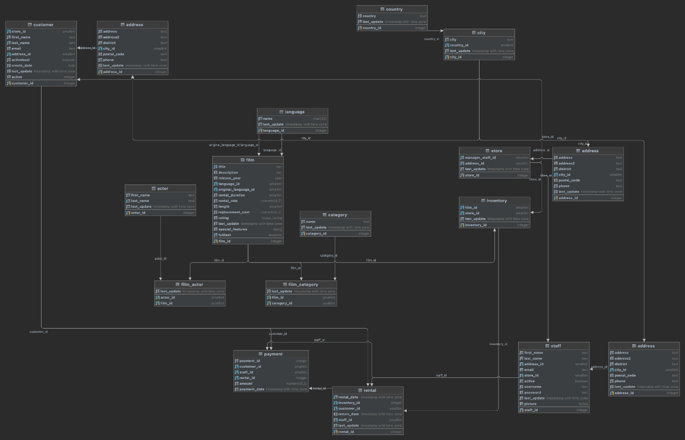
The Pagila database represents a DVD rental business. The database is well-built, small, and adheres to a third normal form (3NF) database schema design. The Pagila database has many objects, including 1 schema, 15 tables, 1 trigger, 7 views, 8 functions, 1 domain, 1 type, 1 aggregate, and 13 sequences. Pagila’s tables contain between 2 and 16K rows.
Pattern 1: Single Schema
Pattern 1: Single Schema is one of the most basic database patterns. There is one database instance containing a single database. That database has a single schema containing all tables and other database objects.

As organizations begin to move from monolithic to microservices architectures, they often retain their monolithic database architecture for some time.

Frequently, the monolithic database’s data model is equally monolithic, lacking proper separation of concerns using simple database constructs such as schemas. The Pagila database is an example of this first pattern. The Pagila database has a single schema containing all database object types, including tables, functions, views, procedures, sequences, and triggers.
To create a copy of the Pagila database, we can use pg_restore to restore any of several publically available custom-format database archive files. If you already have the Pagila database running, simply create a copy with pg_dump.
Below we see the table layout of the Pagila database, which contains the single, default public schema.
-----------+----------+--------+------------
 Instance  | Database | Schema | Table
-----------+----------+--------+------------
 postgres1 | pagila   | public | actor
 postgres1 | pagila   | public | address
 postgres1 | pagila   | public | category
 postgres1 | pagila   | public | city
 postgres1 | pagila   | public | country
 postgres1 | pagila   | public | customer
 postgres1 | pagila   | public | film
 postgres1 | pagila   | public | film_actor
 postgres1 | pagila   | public | film_category
 postgres1 | pagila   | public | inventory
 postgres1 | pagila   | public | language
 postgres1 | pagila   | public | payment
 postgres1 | pagila   | public | rental
 postgres1 | pagila   | public | staff
 postgres1 | pagila   | public | store
Using a single schema to house all tables, especially the public schema is generally considered poor database design. As a database grows in complexity, creating, organizing, managing, and securing dozens, hundreds, or thousands of database objects, including tables, within a single schema becomes impossible. For example, given a single schema, the only way to organize large numbers of database objects is by using lengthy and cryptic naming conventions.
Public Schema
According to the PostgreSQL docs, if tables or other object types are created without specifying a schema name, they are automatically assigned to the default public schema. Every new database contains a public schema. By default, users cannot access any objects in schemas they do not own. To allow that, the schema owner must grant the USAGE privilege on the schema. by default, everyone has CREATE and USAGE privileges on the schema public. These default privileges enable all users to connect to a given database to create objects in its public schema. Some usage patterns call for revoking that privilege, which is a compelling reason not to use the public schema as part of your database design.
Pattern 2: Multiple Schemas
Separating tables and other database objects into multiple schemas is an excellent first step to refactoring a database to support microservices. As application complexity and databases naturally grow over time, schemas to separate functionality by business subdomain or teams will benefit significantly.
According to the PostgreSQL docs, there are several reasons why one might want to use schemas:
- To allow many users to use one database without interfering with each other.
- To organize database objects into logical groups to make them more manageable.
- Third-party applications can be put into separate schemas, so they do not collide with the names of other objects.
Schemas are analogous to directories at the operating system level, except schemas cannot be nested.

With Pattern 2, as an organization continues to decompose its monolithic application architecture to a microservices-based application, it could transition to a schema-per-microservice or similar level or organizational granularity.

Applying Domain-driven Design Principles
Domain-driven design (DDD) is “a software design approach focusing on modeling software to match a domain according to input from that domain’s experts” (Wikipedia). Architects often apply DDD principles to decompose a monolithic application into microservices. For example, a microservice or set of related microservices might represent a Bounded Context. In DDD, a Bounded Context is “a description of a boundary, typically a subsystem or the work of a particular team, within which a particular model is defined and applicable.” (hackernoon.com). Examples of Bounded Context might include Sales, Shipping, and Support.
One technique to apply schemas when refactoring a database is to mirror the Bounded Contexts, which reflect the microservices. For each microservice or set of closely related microservices, there is a schema. Unfortunately, there is no absolute way to define the Bounded Contexts of a Domain, and henceforth, schemas to a database. It depends on many factors, including your application architecture, features, security requirements, and often an organization’s functional team structure.
Reviewing the purpose of each table in the Pagila database and their relationships to each other, we could infer Bounded Contexts, such as Films, Stores, Customers, and Sales. We can represent these Bounded Contexts as schemas within the database as a way to organize the data. The individual tables in a schema mirror DDD concepts, such as aggregates, entities, or value objects.
As shown below, the tables of the Pagila database have been relocated into six new schemas: common, customers, films, sales, staff, and stores. The common schema contains tables with address data references tables in several other schemas. There are now no tables left in the public schema. We will assume other database objects (e.g., functions, views, and triggers) have also been moved and modified if necessary to reflect new table locations.
-----------+----------+-----------+---------------
 Instance  | Database | Schema    | Table
-----------+----------+-----------+---------------
 postgres1 | pagila   | common    | address
 postgres1 | pagila   | common    | city
 postgres1 | pagila   | common    | country
-----------+----------+-----------+---------------
 postgres1 | pagila   | customers | customer
-----------+----------+-----------+---------------
 postgres1 | pagila   | films     | actor
 postgres1 | pagila   | films     | category
 postgres1 | pagila   | films     | film
 postgres1 | pagila   | films     | film_actor
 postgres1 | pagila   | films     | film_category
 postgres1 | pagila   | films     | language
-----------+----------+-----------+---------------
 postgres1 | pagila   | sales     | payment
 postgres1 | pagila   | sales     | rental
-----------+----------+-----------+---------------
 postgres1 | pagila   | staff     | staff
-----------+----------+-----------+---------------
 postgres1 | pagila   | stores    | inventory
 postgres1 | pagila   | stores    | store
By applying schemas, we align tables and other database objects to individual microservices or functional teams that own the microservices and the associated data. Schemas allow us to apply fine-grain access control over objects and data within the database more effectively.

Refactoring other Database Objects
Typically with psql, when moving tables across schemas using an ALTER TABLE...SET SCHEMA... SQL statement, objects such as database views will be updated to the table’s new location. For example, take Pagila’s sales_by_store view. Note the schemas have been automatically updated for multiple tables from their original location in the public schema. The view was also moved to the sales schema.
Splitting Table Data Across Multiple Schemas
When refactoring a database, you may have to split data by replicating table definitions across multiple schemas. Take, for example, Pagila’s address table, which contains the addresses of customers, staff, and stores. The customers.customer, stores.staff, and stores.store all have foreign key relationships with the common.address table. The address table has a foreign key relationship with both the city and country tables. Thus for convenience, the address, city, and country tables were all placed into the common schema in the example above.
Although, at first, storing all the addresses in a single table might appear to be sound database normalization, consider the risks of having the address table’s data exposed. The store addresses are not considered sensitive data. However, the home addresses of customers and staff are likely considered sensitive personally identifiable information (PII). Also, consider as an application evolves, you may have fields unique to one type of address that does not apply to other categories of addresses. The table definitions for a store’s address may be defined differently than the address of a customer. For example, we might choose to add a county column to the customers.address table for e-commerce tax purposes, or an on_site_parking boolean column to the stores.address table.
In the example below, a new staff schema was added. The address table definition was replicated in the customers, staff, and stores schemas. The assumption is that the mixed address data in the original table was distributed to the appropriate address tables. Note the way schemas help us avoid table name collisions.
-----------+----------+-----------+---------------
 Instance  | Database | Schema    | Table
-----------+----------+-----------+---------------
 postgres1 | pagila   | common    | city
 postgres1 | pagila   | common    | country
-----------+----------+-----------+---------------
 postgres1 | pagila   | customers | address
 postgres1 | pagila   | customers | customer
-----------+----------+-----------+---------------
 postgres1 | pagila   | films     | actor
 postgres1 | pagila   | films     | category
 postgres1 | pagila   | films     | film
 postgres1 | pagila   | films     | film_actor
 postgres1 | pagila   | films     | film_category
 postgres1 | pagila   | films     | language
-----------+----------+-----------+---------------
 postgres1 | pagila   | sales     | payment
 postgres1 | pagila   | sales     | rental
-----------+----------+-----------+---------------
 postgres1 | pagila   | staff     | address
 postgres1 | pagila   | staff     | staff
-----------+----------+-----------+---------------
 postgres1 | pagila   | stores    | address
 postgres1 | pagila   | stores    | inventory
 postgres1 | pagila   | stores    | store
To create the new customers.address table, we could use the following SQL statements. The statements to create the other two address tables are nearly identical.
Although we now have two additional tables with identical table definitions, we do not duplicate any data. We could use the following SQL statements to migrate unique address data into the appropriate tables and confirm the results.
Lastly, alter the existing foreign key constraints to point to the new address tables. The SQL statements for the other two address tables are nearly identical.
There is now a reduced risk of exposing sensitive customer or staff data when querying store addresses, and the three address entities can evolve independently. Individual functional teams separately responsible customers, staff, and stores, can own and manage just the data within their domain.
Before dropping the common.address tables, you would still need to modify the remaining database objects that have dependencies on this table, such as views and functions. For example, take Pagila’s sales_by_store view we saw previously. Note line 9, below, the schema of the address table has been updated from common.address to stores.address. The stores.address table only contains addresses of stores, not customers or staff.
Below, we see the final table structure for the Pagila database after refactoring. Tables have been loosely grouped together schema in the diagram.
Pattern 3: Multiple Databases
Similar to how individual schemas allow us to organize tables and other database objects and provide better separation of concerns, we can use databases the same way. For example, we could choose to spread the Pagila data across more than one database within a single RDS database instance. Again, using DDD concepts, while schemas might represent Bounded Contexts, databases most closely align to Domains, which are “spheres of knowledge and activity where the application logic revolves” (hackernoon.com).

With Pattern 3, as an organization continues to refine its microservices-based application architecture, it might find that multiple databases within the same database instance are advantageous to further separate and organize application data.

Let’s assume that the data in the films schema is owned and managed by a completely separate team who should never have access to sensitive data stored in the customers, stores, and sales schemas. According to the PostgreSQL docs, database access permissions are managed using the concept of roles. Depending on how the role is set up, a role can be thought of as either a database user or a group of users.
To provide greater separation of concerns than just schemas, we can create a second, completely separate database within the same RDS database instance for data related to films. With two separate databases, it is easier to create and manage distinct roles and ensure access to customers, stores, or sales data is only accessible to teams that need access.
Below, we see the new layout of tables now spread across two databases within the same RDS database instance. Two new tables, highlighted in bold, are explained below.
-----------+----------+-----------+---------------
 Instance  | Database | Schema    | Table
-----------+----------+-----------+---------------
 postgres1 | pagila   | common    | city
 postgres1 | pagila   | common    | country
-----------+----------+-----------+---------------
 postgres1 | pagila   | customers | address
 postgres1 | pagila   | customers | customer
-----------+----------+-----------+---------------
 postgres1 | pagila   | films     | film
-----------+----------+-----------+---------------
 postgres1 | pagila   | sales     | payment
 postgres1 | pagila   | sales     | rental
-----------+----------+-----------+---------------
 postgres1 | pagila   | staff     | address
 postgres1 | pagila   | staff     | staff
-----------+----------+-----------+---------------
 postgres1 | pagila   | stores    | address
 postgres1 | pagila   | stores    | inventory
 postgres1 | pagila   | stores    | store
-----------+----------+-----------+---------------
 postgres1 | products | films     | actor
 postgres1 | products | films     | category
 postgres1 | products | films     | film
 postgres1 | products | films     | film_actor
 postgres1 | products | films     | film_category
 postgres1 | products | films     | language
 postgres1 | products | films     | outbox
Change Data Capture and the Outbox Pattern
Inserts, updates, and deletes of film data can be replicated between the two databases using several methods, including Change Data Capture (CDC) with the Outbox Pattern. CDC is “a pattern that enables database changes to be monitored and propagated to downstream systems” (RedHat). The Outbox Pattern uses the PostgreSQL database’s ability to perform an commit to two tables atomically using a transaction. Transactions bundles multiple steps into a single, all-or-nothing operation.
In this example, data is written to existing tables in the products.films schema (updated aggregate’s state) as well as a new products.films.outbox table (new domain events), wrapped in a transaction. Using CDC, the domain events from the products.films.outbox table are replicated to the pagila.films.film table. The replication of data between the two databases using CDC is also referred to as eventual consistency.

In this example, films in the pagila.films.film and products.films.outbox tables are represented in a denormalized, aggregated view of a film instead of the original, normalized relational multi-table structure. The table definition of the new pagila.films.film table is very different than that of the original Pagila products.films.films table. A concept such as a film, represented as an aggregate or entity, can be common to multiple Bounded Contexts, yet have a different definition.
Note the Confluent JDBC Source Connector (io.confluent.connect.jdbc.JdbcSourceConnector) used here will not work with PostgreSQL arrays, which would be ideal for one-to-many categories and actors columns. Arrays can be converted to text using ::text or by building value-delimited strings using string_agg aggregate function.
Given this table definition, the resulting data would look as follows.
The existing pagila.stores.inventory table has a foreign key constraint on the the pagila.films.film table. However, the films schema and associated tables have been migrated to the products database’s films schema. To overcome this challenge, we can:
- Create a new
pagila.films.filmtable - Continuously replicate data from the
productsdatabase to thepagila.films.filmtable data using CDC (see below) - Modify the
pagila.stores.inventorytable to take a dependency on the newfilmtable - Drop the duplicate tables and other objects from the
pagila.filmsschema
Debezium and Confluent for CDC
There are several technology choices for performing CDC. For this post, I have used RedHat’s Debezium connector for PostgreSQL and Debezium Outbox Event Router, and Confluent’s JDBC Sink Connector. Below, we see a typical example of a Kafka Connect Source Connector using the Debezium connector for PostgreSQL and a Sink Connector using the Confluent JDBC Sink Connector. The Source Connector streams changes from the products logs, using PostgreSQL’s Write-Ahead Logging (WAL) feature, to an Apache Kafka topic. A corresponding Sink Connector streams the changes from the Kafka topic to the pagila database.
Pattern 4: Multiple Database Instances
At some point in the evolution of a microservices-based application, it might become advantageous to separate the data into multiple database instances using the same database engine. Although managing numerous database instances may require more resources, there are also advantages. Each database instance will have independent connection configurations, roles, and administrators. Each database instance could run different versions of the database engine, and each could be upgraded and maintained independently.

With Pattern 4, as an organization continues to refine its application architecture, it might find that multiple database instances are beneficial to further separate and organize application data.

Below is one possible refactoring of the Pagila database, splitting the data between two database engines. The first database instance, postgres1, contains two databases, pagila and products. The second database instance, postgres2, contains a single database, products.
-----------+----------+-----------+---------------
 Instance  | Database | Schema    | Table
-----------+----------+-----------+---------------
 postgres1 | pagila   | common    | city
 postgres1 | pagila   | common    | country
-----------+----------+-----------+---------------
 postgres1 | pagila   | customers | address
 postgres1 | pagila   | customers | customer
-----------+----------+-----------+---------------
 postgres1 | pagila   | films     | actor
 postgres1 | pagila   | films     | category
 postgres1 | pagila   | films     | film
 postgres1 | pagila   | films     | film_actor
 postgres1 | pagila   | films     | film_category
 postgres1 | pagila   | films     | language
-----------+----------+-----------+---------------
 postgres1 | pagila   | staff     | address
 postgres1 | pagila   | staff     | staff
-----------+----------+-----------+---------------
 postgres1 | pagila   | stores    | address
 postgres1 | pagila   | stores    | inventory
 postgres1 | pagila   | stores    | store
-----------+----------+-----------+---------------
 postgres1 | pagila   | sales     | payment
 postgres1 | pagila   | sales     | rental
-----------+----------+-----------+---------------
 postgres2 | products | films     | actor
 postgres2 | products | films     | category
 postgres2 | products | films     | film
 postgres2 | products | films     | film_actor
 postgres2 | products | films     | film_category
 postgres2 | products | films     | language
Data Replication with CDC
Note the films schema is duplicated between the two databases, shown above. Again, using the CDC allows us to keep the six postgres1.pagila.films tables in sync with the six postgres2.products.films tables using CDC. In this example, we are not using the OutBox Pattern, as used previously in Pattern 3. Instead, we are replicating any changes to any of the tables in postgres2.products.films schema to the corresponding tables in the postgres1.pagila.films schema.

To ensure the tables stay in sync, the tables and other objects in the postgres1.pagila.films schema should be limited to read-only access (SELECT) for all users. The postgres2.products.films tables represent the authoritative source of data, the System of Record (SoR). Any inserts, updates, or deletes, must be made to these tables and replicated using CDC.
Pattern 5: Multiple Database Engines
AWS commonly uses the term ‘purpose-built databases.’ AWS offers over fifteen purpose-built database engines to support diverse data models, including relational, key-value, document, in-memory, graph, time series, wide column, and ledger. There may be instances where using multiple, purpose-built databases makes sense. Using different database engines allows architects to take advantage of the unique characteristics of each engine type to support diverse application requirements.
With Pattern 5, as an organization continues to refine its application architecture, it might choose to leverage multiple, different database engines.

Take for example an application that uses a combination of relational, NoSQL, and in-memory databases to persist data. In addition to PostgreSQL, the application benefits from moving a certain subset of its relational data to a non-relational, high-performance key-value store, such as Amazon DynamoDB. Furthermore, the application implements a database cache using an ultra-fast in-memory database, such as Amazon ElastiCache for Redis.
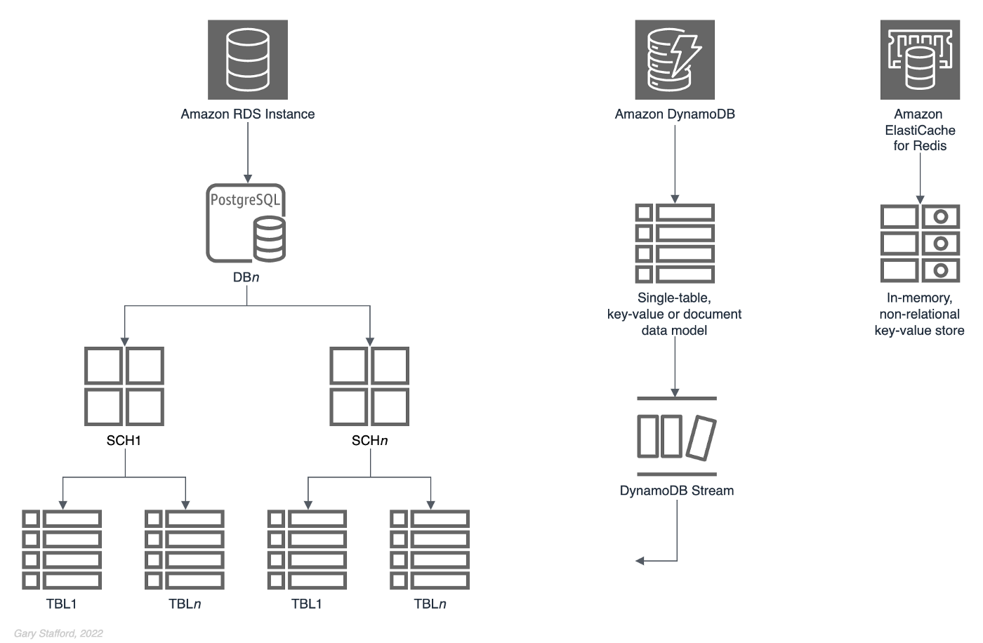
Below is one possible refactoring of the Pagila database, splitting the data between two different database engines, PostgreSQL and Amazon DynamoDB.
-----------+----------+-----------+-----------
 Instance  | Database | Schema    | Table
-----------+----------+-----------+-----------
 postgres1 | pagila   | common    | city
 postgres1 | pagila   | common    | country
-----------+----------+-----------+-----------
 postgres1 | pagila   | customers | address
 postgres1 | pagila   | customers | customer
-----------+----------+-----------+-----------
 postgres1 | pagila   | films     | film
-----------+----------+-----------+-----------
 postgres1 | sales    | sales     | payment
 postgres1 | sales    | sales     | rental
-----------+----------+-----------+-----------
 postgres1 | pagila   | staff     | address
 postgres1 | pagila   | staff     | staff
-----------+----------+-----------+-----------
 postgres1 | pagila   | stores    | address
 postgres1 | pagila   | stores    | film
 postgres1 | pagila   | stores    | inventory
 postgres1 | pagila   | stores    | store
-----------+----------+-----------+-----------
 DynamoDB  |    -     |     -     | Films
The assumption is that based on the application’s access patterns for film data, the application could benefit from the addition of a non-relational, high-performance key-value store. Further, the film-related data entities, such as a film , category, and actor, could be modeled using DynamoDB’s single-table data model architecture. In this model, multiple entity types can be stored in the same table. If necessary, to replicate data back to the PostgreSQL instance from the DynamoBD instance, we can perform CDC with DynamoDB Streams.

Films data model for DynamoDB using NoSQL Workbench
Films data modelCQRS
Command Query Responsibility Segregation (CQRS), a popular software architectural pattern, is another use case for multiple database engines. The CQRS pattern is, as the name implies, “a software design pattern that separates command activities from query activities. In CQRS parlance, a command writes data to a data source. A query reads data from a data source. CQRS addresses the problem of data access performance degradation when applications running at web-scale have too much burden placed on the physical database and the network on which it resides” (RedHat). CQRS commonly uses one database engine optimized for writes and a separate database optimized for reads.

Conclusion
Embracing a microservices-based application architecture may have many business advantages for an organization. However, ignoring the application’s existing databases can negate many of the benefits of microservices. This post examined several common patterns for refactoring relational databases to match a modern microservices-based application architecture.
This blog represents my own viewpoints and not of my employer, Amazon Web Services (AWS). All product names, logos, and brands are the property of their respective owners. All diagrams and illustrations are property of the author.
Java Development with Microsoft SQL Server: Calling Microsoft SQL Server Stored Procedures from Java Applications Using JDBC
Posted by Gary A. Stafford in AWS, Java Development, Software Development, SQL, SQL Server Development on September 9, 2020
Introduction
Enterprise software solutions often combine multiple technology platforms. Accessing an Oracle database via a Microsoft .NET application and vice-versa, accessing Microsoft SQL Server from a Java-based application is common. In this post, we will explore the use of the JDBC (Java Database Connectivity) API to call stored procedures from a Microsoft SQL Server 2017 database and return data to a Java 11-based console application.
The objectives of this post include:
- Demonstrate the differences between using static SQL statements and stored procedures to return data.
- Demonstrate three types of JDBC statements to return data:
Statement,PreparedStatement, andCallableStatement. - Demonstrate how to call stored procedures with input and output parameters.
- Demonstrate how to return single values and a result set from a database using stored procedures.
Why Stored Procedures?
To access data, many enterprise software organizations require their developers to call stored procedures within their code as opposed to executing static T-SQL (Transact-SQL) statements against the database. There are several reasons stored procedures are preferred:
- Optimization: Stored procedures are often written by DBAs or database developers who specialize in database development. They understand the best way to construct queries for optimal performance and minimal load on the database server. Think of it as a developer using an API to interact with the database.
- Safety and Security: Stored procedures are considered safer and more secure than static SQL statements. The stored procedure provides tight control over the content of the queries, preventing malicious or unintentionally destructive code from being executed against the database.
- Error Handling: Stored procedures can contain logic for handling errors before they bubble up to the application layer and possibly to the end-user.
AdventureWorks 2017 Database
For brevity, I will use an existing and well-known Microsoft SQL Server database, AdventureWorks. The AdventureWorks database was originally published by Microsoft for SQL Server 2008. Although a bit dated architecturally, the database comes prepopulated with plenty of data for demonstration purposes.

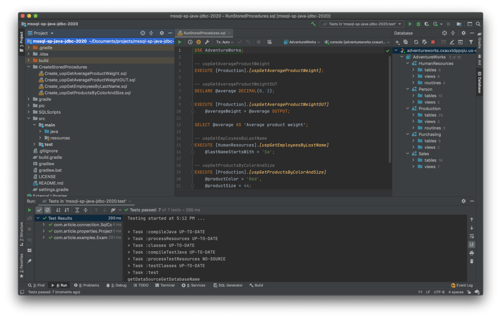
HumanResources schema, one of five schemas within the AdventureWorks databaseFor the demonstration, I have created an Amazon RDS for SQL Server 2017 Express Edition instance on AWS. You have several options for deploying SQL Server, including AWS, Microsoft Azure, Google Cloud, or installed on your local workstation.
There are many methods to deploy the AdventureWorks database to Microsoft SQL Server. For this post’s demonstration, I used the AdventureWorks2017.bak backup file, which I copied to Amazon S3. Then, I enabled and configured the native backup and restore feature of Amazon RDS for SQL Server to import and install the backup.
DROP DATABASE IF EXISTS AdventureWorks;
GO

EXECUTE msdb.dbo.rds_restore_database
     @restore_db_name='AdventureWorks',
     @s3_arn_to_restore_from='arn:aws:s3:::my-bucket/AdventureWorks2017.bak',
     @type='FULL',
     @with_norecovery=0;

-- get task_id from output (e.g. 1)

EXECUTE msdb.dbo.rds_task_status
     @db_name='AdventureWorks',
     @task_id=1;
Install Stored Procedures
For the demonstration, I have added four stored procedures to the AdventureWorks database to use in this post. To follow along, you will need to install these stored procedures, which are included in the GitHub project.

Data Sources, Connections, and Properties
Using the latest Microsoft JDBC Driver 8.4 for SQL Server (ver. 8.4.1.jre11), we create a SQL Server data source, com.microsoft.sqlserver.jdbc.SQLServerDataSource, and database connection, java.sql.Connection. There are several patterns for creating and working with JDBC data sources and connections. This post does not necessarily focus on the best practices for creating or using either. In this example, the application instantiates a connection class, SqlConnection.java, which in turn instantiates the java.sql.Connection and com.microsoft.sqlserver.jdbc.SQLServerDataSource objects. The data source’s properties are supplied from an instance of a singleton class, ProjectProperties.java. This properties class instantiates the java.util.Properties class, which reads values from a configuration properties file, config.properties. On startup, the application creates the database connection, calls each of the example methods, and then closes the connection.
Examples
For each example, I will show the stored procedure, if applicable, followed by the Java method that calls the procedure or executes the static SQL statement. I have left out the data source and connection code in the article. Again, a complete copy of all the code for this article is available on GitHub, including Java source code, SQL statements, helper SQL scripts, and a set of basic JUnit tests.
To run the JUnit unit tests, using Gradle, which the project is based on, use the ./gradlew cleanTest test --warning-mode none command.

To build and run the application, using Gradle, which the project is based on, use the ./gradlew run --warning-mode none command.

Example 1: SQL Statement
Before jumping into stored procedures, we will start with a simple static SQL statement. This example’s method, getAverageProductWeightST, uses the java.sql.Statement class. According to Oracle’s JDBC documentation, the Statement object is used for executing a static SQL statement and returning the results it produces. This SQL statement calculates the average weight of all products in the AdventureWorks database. It returns a solitary double numeric value. This example demonstrates one of the simplest methods for returning data from SQL Server.
/**
 * Statement example, no parameters, returns Integer
 *
 * @return Average weight of all products
 */
public double getAverageProductWeightST() {
    double averageWeight = 0;
    Statement stmt = null;
    ResultSet rs = null;
try {
        stmt = connection.getConnection().createStatement();
        String sql = "WITH Weights_CTE(AverageWeight) AS" +
                "(" +
                "    SELECT [Weight] AS [AverageWeight]" +
                "    FROM [Production].[Product]" +
                "    WHERE [Weight] > 0" +
                "        AND [WeightUnitMeasureCode] = 'LB'" +
                "    UNION" +
                "    SELECT [Weight] * 0.00220462262185 AS [AverageWeight]" +
                "    FROM [Production].[Product]" +
                "    WHERE [Weight] > 0" +
                "        AND [WeightUnitMeasureCode] = 'G')" +
                "SELECT ROUND(AVG([AverageWeight]), 2)" +
                "FROM [Weights_CTE];";
        rs = stmt.executeQuery(sql);
        if (rs.next()) {
            averageWeight = rs.getDouble(1);
        }
    } catch (Exception ex) {
        Logger.getLogger(RunExamples.class.getName()).
                log(Level.SEVERE, null, ex);
    } finally {
        if (rs != null) {
            try {
                rs.close();
            } catch (SQLException ex) {
                Logger.getLogger(RunExamples.class.getName()).
                        log(Level.WARNING, null, ex);
            }
        }
        if (stmt != null) {
            try {
                stmt.close();
            } catch (SQLException ex) {
                Logger.getLogger(RunExamples.class.getName()).
                        log(Level.WARNING, null, ex);
            }
        }
    }
    return averageWeight;
}
Example 2: Prepared Statement
Next, we will execute almost the same static SQL statement as in Example 1. The only change is the addition of the column name, averageWeight. This allows us to parse the results by column name, making the code easier to understand as opposed to using the numeric index of the column as in Example 1.
Also, instead of using the java.sql.Statement class, we use the java.sql.PreparedStatement class. According to Oracle’s documentation, a SQL statement is precompiled and stored in a PreparedStatement object. This object can then be used to execute this statement multiple times efficiently.
/**
 * PreparedStatement example, no parameters, returns Integer
 *
 * @return Average weight of all products
 */
public double getAverageProductWeightPS() {
    double averageWeight = 0;
    PreparedStatement pstmt = null;
    ResultSet rs = null;
try {
        String sql = "WITH Weights_CTE(averageWeight) AS" +
                "(" +
                "    SELECT [Weight] AS [AverageWeight]" +
                "    FROM [Production].[Product]" +
                "    WHERE [Weight] > 0" +
                "        AND [WeightUnitMeasureCode] = 'LB'" +
                "    UNION" +
                "    SELECT [Weight] * 0.00220462262185 AS [AverageWeight]" +
                "    FROM [Production].[Product]" +
                "    WHERE [Weight] > 0" +
                "        AND [WeightUnitMeasureCode] = 'G')" +
                "SELECT ROUND(AVG([AverageWeight]), 2) AS [averageWeight]" +
                "FROM [Weights_CTE];";
        pstmt = connection.getConnection().prepareStatement(sql);
        rs = pstmt.executeQuery();
        if (rs.next()) {
            averageWeight = rs.getDouble("averageWeight");
        }
    } catch (Exception ex) {
        Logger.getLogger(RunExamples.class.getName()).
                log(Level.SEVERE, null, ex);
    } finally {
        if (rs != null) {
            try {
                rs.close();
            } catch (SQLException ex) {
                Logger.getLogger(RunExamples.class.getName()).
                        log(Level.WARNING, null, ex);
            }
        }
        if (pstmt != null) {
            try {
                pstmt.close();
            } catch (SQLException ex) {
                Logger.getLogger(RunExamples.class.getName()).
                        log(Level.WARNING, null, ex);
            }
        }
    }
    return averageWeight;
}
Example 3: Callable Statement
In this example, the average product weight query has been moved into a stored procedure. The procedure is identical in functionality to the static statement in the first two examples. To call the stored procedure, we use the java.sql.CallableStatement class. According to Oracle’s documentation, the CallableStatement extends PreparedStatement. It is the interface used to execute SQL stored procedures. The CallableStatement accepts both input and output parameters; however, this simple example does not use either. Like the previous two examples, the procedure returns a double numeric value.
CREATE OR
ALTER PROCEDURE [Production].[uspGetAverageProductWeight]
AS
BEGIN
  SET NOCOUNT ON;
WITH
    Weights_CTE(AverageWeight)
    AS
    (
        SELECT [Weight] AS [AverageWeight]
        FROM [Production].[Product]
        WHERE [Weight] > 0
          AND [WeightUnitMeasureCode] = 'LB'
      UNION
        SELECT [Weight] * 0.00220462262185 AS [AverageWeight]
        FROM [Production].[Product]
        WHERE [Weight] > 0
          AND [WeightUnitMeasureCode] = 'G'
    )
  SELECT ROUND(AVG([AverageWeight]), 2)
  FROM [Weights_CTE];
END
GO
The calling Java method is shown below.
/**
 * CallableStatement, no parameters, returns Integer
 *
 * @return Average weight of all products
 */
public double getAverageProductWeightCS() {
    CallableStatement cstmt = null;
    double averageWeight = 0;
    ResultSet rs = null;
    try {
        cstmt = connection.getConnection().prepareCall(
                "{call [Production].[uspGetAverageProductWeight]}");
        cstmt.execute();
        rs = cstmt.getResultSet();
        if (rs.next()) {
            averageWeight = rs.getDouble(1);
        }
    } catch (Exception ex) {
        Logger.getLogger(RunExamples.class.getName()).
                log(Level.SEVERE, null, ex);
    } finally {
        if (rs != null) {
            try {
                rs.close();
            } catch (SQLException ex) {
                Logger.getLogger(RunExamples.class.getName()).
                        log(Level.SEVERE, null, ex);
            }
        }
        if (cstmt != null) {
            try {
                cstmt.close();
            } catch (SQLException ex) {
                Logger.getLogger(RunExamples.class.getName()).
                        log(Level.WARNING, null, ex);
            }
        }
    }
    return averageWeight;
}
Example 4: Calling a Stored Procedure with an Output Parameter
In this example, we use almost the same stored procedure as in Example 3. The only difference is the inclusion of an output parameter. This time, instead of returning a result set with a value in a single unnamed column, the column has a name, averageWeight. We can now call that column by name when retrieving the value.
The stored procedure patterns found in Examples 3 and 4 are both commonly used. One procedure uses an output parameter, and one not, both return the same value(s). You can use the CallableStatement to for either type.
CREATE OR
ALTER PROCEDURE [Production].[uspGetAverageProductWeightOUT]@averageWeight DECIMAL(8, 2) OUT
AS
BEGIN
  SET NOCOUNT ON;
WITH
    Weights_CTE(AverageWeight)
    AS
    (
        SELECT [Weight] AS [AverageWeight]
        FROM [Production].[Product]
        WHERE [Weight] > 0
          AND [WeightUnitMeasureCode] = 'LB'
      UNION
        SELECT [Weight] * 0.00220462262185 AS [AverageWeight]
        FROM [Production].[Product]
        WHERE [Weight] > 0
          AND [WeightUnitMeasureCode] = 'G'
    )
  SELECT @averageWeight = ROUND(AVG([AverageWeight]), 2)
  FROM [Weights_CTE];
END
GO
The calling Java method is shown below.
/**
 * CallableStatement example, (1) output parameter, returns Integer
 *
 * @return Average weight of all products
 */
public double getAverageProductWeightOutCS() {
    CallableStatement cstmt = null;
    double averageWeight = 0;
try {
        cstmt = connection.getConnection().prepareCall(
                "{call [Production].[uspGetAverageProductWeightOUT](?)}");
        cstmt.registerOutParameter("averageWeight", Types.DECIMAL);
        cstmt.execute();
        averageWeight = cstmt.getDouble("averageWeight");
    } catch (Exception ex) {
        Logger.getLogger(RunExamples.class.getName()).
                log(Level.SEVERE, null, ex);
    } finally {
        if (cstmt != null) {
            try {
                cstmt.close();
            } catch (SQLException ex) {
                Logger.getLogger(RunExamples.class.getName()).
                        log(Level.WARNING, null, ex);
            }
        }
    }
    return averageWeight;
}
Example 5: Calling a Stored Procedure with an Input Parameter
In this example, the procedure returns a result set, java.sql.ResultSet, of employees whose last name starts with a particular sequence of characters (e.g., ‘M’ or ‘Sa’). The sequence of characters is passed as an input parameter, lastNameStartsWith, to the stored procedure using the CallableStatement.
The method making the call iterates through the rows of the result set returned by the stored procedure, concatenating multiple columns to form the employee’s full name as a string. Each full name string is then added to an ordered collection of strings, a List<String> object. The List instance is returned by the method. You will notice this procedure takes a little longer to run because of the use of the LIKE operator. The database server has to perform pattern matching on each last name value in the table to determine the result set.
CREATE OR
ALTER PROCEDURE [HumanResources].[uspGetEmployeesByLastName]
@lastNameStartsWith VARCHAR(20) = 'A'
AS
BEGIN
  SET NOCOUNT ON;
SELECT p.[FirstName], p.[MiddleName], p.[LastName], p.[Suffix], e.[JobTitle], m.[EmailAddress]
  FROM [HumanResources].[Employee] AS e
    LEFT JOIN [Person].[Person] p ON e.[BusinessEntityID] = p.[BusinessEntityID]
    LEFT JOIN [Person].[EmailAddress] m ON e.[BusinessEntityID] = m.[BusinessEntityID]
  WHERE e.[CurrentFlag] = 1
    AND p.[PersonType] = 'EM'
    AND p.[LastName] LIKE @lastNameStartsWith + '%'
  ORDER BY p.[LastName], p.[FirstName], p.[MiddleName]
END
GO
The calling Java method is shown below.
/**
 * CallableStatement example, (1) input parameter, returns ResultSet
 *
 * @param lastNameStartsWith
 * @return List of employee names
 */
public List<String> getEmployeesByLastNameCS(String lastNameStartsWith) {
CallableStatement cstmt = null;
    ResultSet rs = null;
    List<String> employeeFullName = new ArrayList<>();
try {
        cstmt = connection.getConnection().prepareCall(
                "{call [HumanResources].[uspGetEmployeesByLastName](?)}",
                ResultSet.TYPE_SCROLL_INSENSITIVE,
                ResultSet.CONCUR_READ_ONLY);
cstmt.setString("lastNameStartsWith", lastNameStartsWith);
        boolean results = cstmt.execute();
        int rowsAffected = 0;
// Protects against lack of SET NOCOUNT in stored procedure
        while (results || rowsAffected != -1) {
            if (results) {
                rs = cstmt.getResultSet();
                break;
            } else {
                rowsAffected = cstmt.getUpdateCount();
            }
            results = cstmt.getMoreResults();
        }
        while (rs.next()) {
            employeeFullName.add(
                    rs.getString("LastName") + ", "
                            + rs.getString("FirstName") + " "
                            + rs.getString("MiddleName"));
        }
    } catch (Exception ex) {
        Logger.getLogger(RunExamples.class.getName()).
                log(Level.SEVERE, null, ex);
    } finally {
        if (rs != null) {
            try {
                rs.close();
            } catch (SQLException ex) {
                Logger.getLogger(RunExamples.class.getName()).
                        log(Level.WARNING, null, ex);
            }
        }
        if (cstmt != null) {
            try {
                cstmt.close();
            } catch (SQLException ex) {
                Logger.getLogger(RunExamples.class.getName()).
                        log(Level.WARNING, null, ex);
            }
        }
    }
    return employeeFullName;
}
Example 6: Converting a Result Set to Ordered Collection of Objects
In this last example, we pass two input parameters, productColor and productSize, to a slightly more complex stored procedure. The stored procedure returns a result set containing several columns of product information. This time, the example’s method iterates through the result set returned by the procedure and constructs an ordered collection of products, List<Product> object. The Product objects in the list are instances of the Product.java POJO class. The method converts each results set’s row’s field value into a Product property (e.g., Product.Size, Product.Model). Using a collection is a common method for persisting data from a result set in an application.
CREATE OR
ALTER PROCEDURE [Production].[uspGetProductsByColorAndSize]
  @productColor VARCHAR(20),
  @productSize INTEGER
AS
BEGIN
  SET NOCOUNT ON;
SELECT p.[ProductNumber], m.[Name] AS [Model], p.[Name] AS [Product], p.[Color], p.[Size]
  FROM [Production].[ProductModel] AS m
    INNER JOIN
    [Production].[Product] AS p ON m.[ProductModelID] = p.[ProductModelID]
  WHERE (p.[Color] = @productColor)
    AND (p.[Size] = @productSize)
  ORDER BY p.[ProductNumber], [Model], [Product]
END
GO
The calling Java method is shown below.
/**
 * CallableStatement example, (2) input parameters, returns ResultSet
 *
 * @param color
 * @param size
 * @return List of Product objects
 */
public List<Product> getProductsByColorAndSizeCS(String color, String size) {
CallableStatement cstmt = null;
    ResultSet rs = null;
    List<Product> productList = new ArrayList<>();
try {
        cstmt = connection.getConnection().prepareCall(
                "{call [Production].[uspGetProductsByColorAndSize](?, ?)}",
                ResultSet.TYPE_SCROLL_INSENSITIVE,
                ResultSet.CONCUR_READ_ONLY);
cstmt.setString("productColor", color);
        cstmt.setString("productSize", size);
        boolean results = cstmt.execute();
        int rowsAffected = 0;
// Protects against lack of SET NOCOUNT in stored procedure
        while (results || rowsAffected != -1) {
            if (results) {
                rs = cstmt.getResultSet();
                break;
            } else {
                rowsAffected = cstmt.getUpdateCount();
            }
            results = cstmt.getMoreResults();
        }
while (rs.next()) {
            Product product = new Product(
                    rs.getString("Product"),
                    rs.getString("ProductNumber"),
                    rs.getString("Color"),
                    rs.getString("Size"),
                    rs.getString("Model"));
            productList.add(product);
        }
    } catch (Exception ex) {
        Logger.getLogger(RunExamples.class.getName()).
                log(Level.SEVERE, null, ex);
    } finally {
        if (rs != null) {
            try {
                rs.close();
            } catch (SQLException ex) {
                Logger.getLogger(RunExamples.class.getName()).
                        log(Level.WARNING, null, ex);
            }
        }
        if (cstmt != null) {
            try {
                cstmt.close();
            } catch (SQLException ex) {
                Logger.getLogger(RunExamples.class.getName()).
                        log(Level.WARNING, null, ex);
            }
        }
    }
    return productList;
}
Proper T-SQL: Schema Reference and Brackets
You will notice in all T-SQL statements, I refer to the schema as well as the table or stored procedure name (e.g., {call [Production].[uspGetAverageProductWeightOUT](?)}). According to Microsoft, it is always good practice to refer to database objects by a schema name and the object name, separated by a period; that even includes the default schema (e.g., dbo).
You will also notice I wrap the schema and object names in square brackets (e.g., SELECT [ProductNumber] FROM [Production].[ProductModel]). The square brackets are to indicate that the name represents an object and not a reserved word (e.g, CURRENT or NATIONAL). By default, SQL Server adds these to make sure the scripts it generates run correctly.
Running the Examples
The application will display the name of the method being called, a description, the duration of time it took to retrieve the data, and the results returned by the method.
Below, we see the results.

SQL Statement Performance
This post is certainly not about SQL performance, demonstrated by the fact I am only using Amazon RDS for SQL Server 2017 Express Edition on a single, very underpowered db.t2.micro Amazon RDS instance types. However, I have added a timer feature, ProcessTimer.java class, to capture the duration of time each example takes to return data, measured in milliseconds. The ProcessTimer.java class is part of the project code. Using the timer, you should observe significant differences between the first run and proceeding runs of the application for several of the called methods. The time difference is a result of several factors, primarily pre-compilation of the SQL statements and SQL Server plan caching.
The effects of these two factors are easily demonstrated by clearing the SQL Server plan cache (see SQL script below) using DBCC (Database Console Commands) statements. and then running the application twice in a row. The second time, pre-compilation and plan caching should result in significantly faster times for the prepared statements and callable statements, in Examples 2–6. In the two random runs shown below, we see up to a 497% improvement in query time.
USE AdventureWorks;
DBCC FREESYSTEMCACHE('SQL Plans');
GO
CHECKPOINT;
GO
-- Impossible to run with Amazon RDS for Microsoft SQL Server on AWS
-- DBCC DROPCLEANBUFFERS;
-- GO
The first run results are shown below.
SQL SERVER STATEMENT EXAMPLES
======================================
Method: GetAverageProductWeightST
Description: Statement, no parameters, returns Integer
Duration (ms): 122
Results: Average product weight (lb): 12.43
---
Method: GetAverageProductWeightPS
Description: PreparedStatement, no parameters, returns Integer
Duration (ms): 146
Results: Average product weight (lb): 12.43
---
Method: GetAverageProductWeightCS
Description: CallableStatement, no parameters, returns Integer
Duration (ms): 72
Results: Average product weight (lb): 12.43
---
Method: GetAverageProductWeightOutCS
Description: CallableStatement, (1) output parameter, returns Integer
Duration (ms): 623
Results: Average product weight (lb): 12.43
---
Method: GetEmployeesByLastNameCS
Description: CallableStatement, (1) input parameter, returns ResultSet
Duration (ms): 830
Results: Last names starting with 'Sa': 7
         Last employee found: Sandberg, Mikael Q
---
Method: GetProductsByColorAndSizeCS
Description: CallableStatement, (2) input parameter, returns ResultSet
Duration (ms): 427
Results: Products found (color: 'Red', size: '44'): 7
         First product: Road-650 Red, 44 (BK-R50R-44)
---
The second run results are shown below.
SQL SERVER STATEMENT EXAMPLES
======================================
Method: GetAverageProductWeightST
Description: Statement, no parameters, returns Integer
Duration (ms): 116
Results: Average product weight (lb): 12.43
---
Method: GetAverageProductWeightPS
Description: PreparedStatement, no parameters, returns Integer
Duration (ms): 89
Results: Average product weight (lb): 12.43
---
Method: GetAverageProductWeightCS
Description: CallableStatement, no parameters, returns Integer
Duration (ms): 80
Results: Average product weight (lb): 12.43
---
Method: GetAverageProductWeightOutCS
Description: CallableStatement, (1) output parameter, returns Integer
Duration (ms): 340
Results: Average product weight (lb): 12.43
---
Method: GetEmployeesByLastNameCS
Description: CallableStatement, (1) input parameter, returns ResultSet
Duration (ms): 139
Results: Last names starting with 'Sa': 7
         Last employee found: Sandberg, Mikael Q
---
Method: GetProductsByColorAndSizeCS
Description: CallableStatement, (2) input parameter, returns ResultSet
Duration (ms): 208
Results: Products found (color: 'Red', size: '44'): 7
         First product: Road-650 Red, 44 (BK-R50R-44)
---
Conclusion
This post has demonstrated several methods for querying and calling stored procedures from a SQL Server 2017 database using JDBC with the Microsoft JDBC Driver 8.4 for SQL Server. Although the examples are quite simple, the same patterns can be used with more complex stored procedures, with multiple input and output parameters, which not only select, but insert, update, and delete data.
There are some limitations of the Microsoft JDBC Driver for SQL Server you should be aware of by reading the documentation. However, for most tasks that require database interaction, the Driver provides adequate functionality with SQL Server.
This blog represents my own viewpoints and not of my employer, Amazon Web Services.
Getting Started with PostgreSQL using Amazon RDS, CloudFormation, pgAdmin, and Python
Posted by Gary A. Stafford in AWS, Cloud, Python, Software Development on August 9, 2019
Introduction
In the following post, we will explore how to get started with Amazon Relational Database Service (RDS) for PostgreSQL. CloudFormation will be used to build a PostgreSQL master database instance and a single read replica in a new VPC. AWS Systems Manager Parameter Store will be used to store our CloudFormation configuration values. Amazon RDS Event Notifications will send text messages to our mobile device to let us know when the RDS instances are ready for use. Once running, we will examine a variety of methods to interact with our database instances, including pgAdmin, Adminer, and Python.
Technologies
The primary technologies used in this post include the following.
PostgreSQL
 According to its website, PostgreSQL, commonly known as Postgres, is the world’s most advanced Open Source relational database. Originating at UC Berkeley in 1986, PostgreSQL has more than 30 years of active core development. PostgreSQL has earned a strong reputation for its proven architecture, reliability, data integrity, robust feature set, extensibility. PostgreSQL runs on all major operating systems and has been ACID-compliant since 2001.
Amazon RDS for PostgreSQL
 According to Amazon, Amazon Relational Database Service (RDS) provides six familiar database engines to choose from, including Amazon Aurora, PostgreSQL, MySQL, MariaDB, Oracle Database, and SQL Server. RDS is available on several database instance types - optimized for memory, performance, or I/O.
Amazon RDS for PostgreSQL makes it easy to set up, operate, and scale PostgreSQL deployments in the cloud. Amazon RDS supports the latest PostgreSQL version 11, which includes several enhancements to performance, robustness, transaction management, query parallelism, and more.
AWS CloudFormation

According to Amazon, CloudFormation provides a common language to describe and provision all the infrastructure resources within AWS-based cloud environments. CloudFormation allows you to use a JSON- or YAML-based template to model and provision all the resources needed for your applications across all AWS regions and accounts, in an automated and secure manner.
Demonstration
Architecture
Below, we see an architectural representation of what will be built in the demonstration. This is not a typical three-tier AWS architecture, wherein the RDS instances would be placed in private subnets (data tier) and accessible only by the application tier, running on AWS. The architecture for the demonstration is designed for interacting with RDS through external database clients such as pgAdmin, and applications like our local Python scripts, detailed later in the post.

Source Code
All source code for this post is available on GitHub in a single public repository, postgres-rds-demo.
.
├── LICENSE.md
├── README.md
├── cfn-templates
│   ├── event.template
│   ├── rds.template
├── parameter_store_values.sh
├── python-scripts
│   ├── create_pagila_data.py
│   ├── database.ini
│   ├── db_config.py
│   ├── query_postgres.py
│   ├── requirements.txt
│   └── unit_tests.py
├── sql-scripts
│   ├── pagila-insert-data.sql
│   └── pagila-schema.sql
└── stack.yml
To clone the GitHub repository, execute the following command.
git clone --branch master --single-branch --depth 1 --no-tags \
  https://github.com/garystafford/aws-rds-postgres.git
Prerequisites
For this demonstration, I will assume you already have an AWS account. Further, that you have the latest copy of the AWS CLI and Python 3 installed on your development machine. Optionally, for pgAdmin and Adminer, you will also need to have Docker installed.
Steps
In this demonstration, we will perform the following steps.
- Put CloudFormation configuration values in Parameter Store;
- Execute CloudFormation templates to create AWS resources;
- Execute SQL scripts using Python to populate the new database with sample data;
- Configure pgAdmin and Python connections to RDS PostgreSQL instances;
AWS Systems Manager Parameter Store
With AWS, it is typical to use services like AWS Systems Manager Parameter Store and AWS Secrets Manager to store overt, sensitive, and secret configuration values. These values are utilized by your code, or from AWS services like CloudFormation. Parameter Store allows us to follow the proper twelve-factor, cloud-native practice of separating configuration from code.
To demonstrate the use of Parameter Store, we will place a few of our CloudFormation configuration items into Parameter Store. The demonstration’s GitHub repository includes a shell script, parameter_store_values.sh, which will put the necessary parameters into Parameter Store.
Below, we see several of the demo’s configuration values, which have been put into Parameter Store.

SecureString
Whereas our other parameters are stored in Parameter Store as String datatypes, the database’s master user password is stored as a SecureString data-type. Parameter Store uses an AWS Key Management Service (KMS) customer master key (CMK) to encrypt the SecureString parameter value.

SMS Text Alert Option
Before running the Parameter Store script, you will need to change the /rds_demo/alert_phone parameter value in the script (shown below) to your mobile device number, including country code, such as ‘+12038675309’. Amazon SNS will use it to send SMS messages, using Amazon RDS Event Notification. If you don’t want to use this messaging feature, simply ignore this parameter and do not execute the event.template CloudFormation template in the proceeding step.
aws ssm put-parameter \
  --name /rds_demo/alert_phone \
  --type String \
  --value "your_phone_number_here" \
  --description "RDS alert SMS phone number" \
  --overwrite
Run the following command to execute the shell script, parameter_store_values.sh, which will put the necessary parameters into Parameter Store.
sh ./parameter_store_values.sh
CloudFormation Templates
The GitHub repository includes two CloudFormation templates, cfn-templates/event.template and cfn-templates/rds.template. This event template contains two resources, which are an AWS SNS Topic and an AWS RDS Event Subscription. The RDS template also includes several resources, including a VPC, Internet Gateway, VPC security group, two public subnets, one RDS master database instance, and an AWS RDS Read Replica database instance.
The resources are split into two CloudFormation templates so we can create the notification resources, first, independently of creating or deleting the RDS instances. This will ensure we get all our SMS alerts about both the creation and deletion of the databases.
Template Parameters
The two CloudFormation templates contain a total of approximately fifteen parameters. For most, you can use the default values I have set or chose to override them. Four of the parameters will be fulfilled from Parameter Store. Of these, the master database password is treated slightly differently because it is secure (encrypted in Parameter Store). Below is a snippet of the template showing both types of parameters. The last two are fulfilled from Parameter Store.
DBInstanceClass:
  Type: String
  Default: "db.t3.small"
DBStorageType:
  Type: String
  Default: "gp2"
DBUser:
  Type: String
  Default: "{{resolve:ssm:/rds_demo/master_username:1}}"
DBPassword:
  Type: String
  Default: "{{resolve:ssm-secure:/rds_demo/master_password:1}}"
  NoEcho: True
Choosing the default CloudFormation parameter values will result in two minimally-configured RDS instances running the PostgreSQL 11.4 database engine on a db.t3.small instance with 10 GiB of General Purpose (SSD) storage. The db.t3 DB instance is part of the latest generation burstable performance instance class. The master instance is not configured for Multi-AZ high availability. However, the master and read replica each run in a different Availability Zone (AZ) within the same AWS Region.
Parameter Versioning
When placing parameters into Parameter Store, subsequent updates to a parameter result in the version number of that parameter being incremented. Note in the examples above, the version of the parameter is required by CloudFormation, here, ‘1’. If you chose to update a value in Parameter Store, thus incrementing the parameter’s version, you will also need to update the corresponding version number in the CloudFormation template’s parameter.
{
    "Parameter": {
        "Name": "/rds_demo/rds_username",
        "Type": "String",
        "Value": "masteruser",
        "Version": 1,
        "LastModifiedDate": 1564962073.774,
        "ARN": "arn:aws:ssm:us-east-1:1234567890:parameter/rds_demo/rds_username"
    }
}
Validating Templates
Although I have tested both templates, I suggest validating the templates yourself, as you usually would for any CloudFormation template you are creating. You can use the AWS CLI CloudFormation validate-template CLI command to validate the template. Alternately, or I suggest additionally, you can use CloudFormation Linter, cfn-lint command.
aws cloudformation validate-template \
  --template-body file://cfn-templates/rds.template

cfn-lint -t cfn-templates/cfn-templates/rds.template
Create the Stacks
To execute the first CloudFormation template and create a CloudFormation Stack containing the two event notification resources, run the following create-stack CLI command.
aws cloudformation create-stack \
  --template-body file://cfn-templates/event.template \
  --stack-name RDSEventDemoStack
The first stack only takes less than one minute to create. Using the AWS CloudFormation Console, make sure the first stack completes successfully before creating the second stack with the command, below.
aws cloudformation create-stack \
  --template-body file://cfn-templates/rds.template \
  --stack-name RDSDemoStack

Wait for my Text
In my tests, the CloudFormation RDS stack takes an average of 25–30 minutes to create and 15–20 minutes to delete, which can seem like an eternity. You could use the AWS CloudFormation console (shown below) or continue to use the CLI to follow the progress of the RDS stack creation.

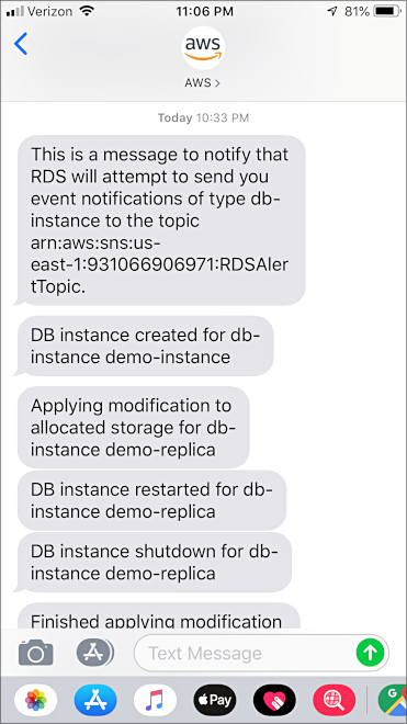
However, if you recall, the CloudFormation event template creates an AWS RDS Event Subscription. This resource will notify us when the databases are ready by sending text messages to our mobile device.

In the CloudFormation events template, the RDS Event Subscription is configured to generate Amazon Simple Notification Service (SNS) notifications for several specific event types, including RDS instance creation and deletion.
  MyEventSubscription:
    Properties:
      Enabled: true
      EventCategories:
        - availability
        - configuration change
        - creation
        - deletion
        - failover
        - failure
        - recovery
      SnsTopicArn:
        Ref: MyDBSNSTopic
      SourceType: db-instance
    Type: AWS::RDS::EventSubscription
Amazon SNS will send SMS messages to the mobile number you placed into Parameter Store. Below, we see messages generated during the creation of the two instances, displayed on an Apple iPhone.
Amazon RDS Dashboard
Once the RDS CloudFormation stack has successfully been built, the easiest way to view the results is using the Amazon RDS Dashboard, as shown below. Here we see both the master and read replica instances have been created and are available for our use.

The RDS dashboard offers CloudWatch monitoring of each RDS instance.

The RDS dashboard also provides detailed configuration information about each RDS instance.

The RDS dashboard’s Connection & security tab is where we can obtain connection information about our RDS instances, including the RDS instance’s endpoints. Endpoints information will be required in the next part of the demonstration.

Sample Data
Now that we have our PostgreSQL database instance and read replica successfully provisioned and configured on AWS, with an empty database, we need some test data. There are several sources of sample PostgreSQL databases available on the internet to explore. We will use the Pagila sample movie rental database by pgFoundry. Although the database is several years old, it provides a relatively complex relational schema (table relationships shown below) and plenty of sample data to query, about 100 database objects and 46K rows of data.

In the GitHub repository, I have included the two Pagila database SQL scripts required to install the sample database’s data structures (DDL), sql-scripts/pagila-schema.sql, and the data itself (DML), sql-scripts/pagila-insert-data.sql.
To execute the Pagila SQL scripts and install the sample data, I have included a Python script. If you do not want to use Python, you can skip to the Adminer section of this post. Adminer also has the capability to import SQL scripts.
Before running any of the included Python scripts, you will need to install the required Python packages and configure the database.ini file.
Python Packages
To install the required Python packages using the supplied python-scripts/requirements.txt file, run the below commands.
cd python-scripts
pip3 install --upgrade -r requirements.txt
We are using two packages, psycopg2 and configparser, for the scripts. Psycopg is a PostgreSQL database adapter for Python. According to their website, Psycopg is the most popular PostgreSQL database adapter for the Python programming language. The configparser module allows us to read configuration from files similar to Microsoft Windows INI files. The unittest package is required for a set of unit tests includes the project, but not discussed as part of the demo.

Database Configuration
The python-scripts/database.ini file, read by configparser, provides the required connection information to our RDS master and read replica instance’s databases. Use the input parameters and output values from the CloudFormation RDS template, or the Amazon RDS Dashboard to obtain the required connection information, as shown in the example, below. Your host values will be unique for your master and read replica. The host values are the instance’s endpoint, listed in the RDS Dashboard’s Configuration tab.
[docker]
host=localhost
port=5432
database=pagila
user=masteruser
password=5up3r53cr3tPa55w0rd

[master]
host=demo-instance.dkfvbjrazxmd.us-east-1.rds.amazonaws.com
port=5432
database=pagila
user=masteruser
password=5up3r53cr3tPa55w0rd

[replica]
host=demo-replica.dkfvbjrazxmd.us-east-1.rds.amazonaws.com
port=5432
database=pagila
user=masteruser
password=5up3r53cr3tPa55w0rd
With the INI file configured, run the following command, which executes a supplied Python script, python-scripts/create_pagila_data.py, to create the data structure and insert sample data into the master RDS instance’s Pagila database. The database will be automatically replicated to the RDS read replica instance. From my local laptop, I found the Python script takes approximately 40 seconds to create all 100 database objects and insert 46K rows of movie rental data. That is compared to about 13 seconds locally, using a Docker-based instance of PostgreSQL.
python3 ./create_pagila_data.py --instance master
The Python script’s primary function, create_pagila_db(), reads and executes the two external SQL scripts.
def create_pagila_db():
    """
    Creates Pagila database by running DDL and DML scripts
    """

    try:
        global conn
        with conn:
            with conn.cursor() as curs:
                curs.execute(open("../sql-scripts/pagila-schema.sql", "r").read())
                curs.execute(open("../sql-scripts/pagila-insert-data.sql", "r").read())
                conn.commit()
                print('Pagila SQL scripts executed')
    except (psycopg2.OperationalError, psycopg2.DatabaseError, FileNotFoundError) as err:
        print(create_pagila_db.__name__, err)
        close_conn()
        exit(1)
If the Python script executes correctly, you should see output indicating there are now 28 tables in our master RDS instance’s database.

pgAdmin
pgAdmin is a favorite tool for interacting with and managing PostgreSQL databases. According to its website, pgAdmin is the most popular and feature-rich Open Source administration and development platform for PostgreSQL.
The project includes an optional Docker Swarm stack.yml file. The stack will create a set of three Docker containers, including a local copy of PostgreSQL 11.4, Adminer, and pgAdmin 4. Having a local copy of PostgreSQL, using the official Docker image, is helpful for development and trouble-shooting RDS issues.

Use the following commands to deploy the Swarm stack.
# create stack
docker swarm init
docker stack deploy -c stack.yml postgres

# get status of new containers
docker stack ps postgres --no-trunc
docker container ls
If you do not want to spin up the whole Docker Swarm stack, you could use the docker run command to create just a single pgAdmin Docker container. The pgAdmin 4 Docker image being used is the image recommended by pgAdmin.
docker pull dpage/pgadmin4

docker run -p 81:80 \
  -e "PGADMIN_DEFAULT_EMAIL=user@domain.com" \
  -e "PGADMIN_DEFAULT_PASSWORD=SuperSecret" \
  -d dpage/pgadmin4

docker container ls | grep pgadmin4
Database Server Configuration
Once pgAdmin is up and running, we can configure the master and read replica database servers (RDS instances) using the connection string information from your database.ini file or from the Amazon RDS Dashboard. Below, I am configuring the master RDS instance (server).

With that task complete, below, we see the master RDS instance and the read replica, as well as my local Docker instance configured in pgAdmin (left side of screengrab). Note how the Pagila database has been replicated automatically, from the RDS master to the read replica instance.

Building SQL Queries
Switching to the Query tab, we can run regular SQL queries against any of the database instances. Below, I have run a simple SELECT query against the master RDS instance’s Pagila database, returning the complete list of movie titles, along with their genre and release date.

The pgAdmin Query tool even includes an Explain tab to view a graphical representation of the same query, very useful for optimization. Here we see the same query, showing an analysis of the execution order. A popup window displays information about the selected object.

Query the Read Replica
To demonstrate the use of the read replica, below I’ve run the same query against the RDS read replica’s copy of the Pagila database. Any schema and data changes against the master instance are replicated to the read replica(s).

Adminer
Adminer is another good general-purpose database management tool, similar to pgAdmin, but with a few different capabilities. According to its website, with Adminer, you get a tidy user interface, rich support for multiple databases, performance, and security, all from a single PHP file. Adminer is my preferred tool for database admin tasks. Amazingly, Adminer works with MySQL, MariaDB, PostgreSQL, SQLite, MS SQL, Oracle, SimpleDB, Elasticsearch, and MongoDB.
Below, we see the Pagila database’s tables and views displayed in Adminer, along with some useful statistical information about each database object.

Similar to pgAdmin, we can also run queries, along with other common development and management tasks, from within the Adminer interface.

Import Pagila with Adminer
Another great feature of Adminer is the ability to easily import and export data. As an alternative to Python, you could import the Pagila data using Adminer’s SQL file import function. Below, you see an example of importing the Pagila database objects into the Pagila database, using the file upload function.

IDE
For writing my AWS infrastructure as code files and Python scripts, I prefer JetBrains PyCharm Professional Edition (v19.2). PyCharm, like all the JetBrains IDEs, has the ability to connect to and manage PostgreSQL database. You can write and run SQL queries, including the Pagila SQL import scripts. Microsoft Visual Studio Code is another excellent, free choice, available on multiple platforms.

Python and RDS
Although our IDE, pgAdmin, and Adminer are useful to build and test our queries, ultimately, we still need to connect to the Amazon RDS PostgreSQL instances and perform data manipulation from our application code. The GitHub repository includes a sample python script, python-scripts/query_postgres.py. This script uses the same Python packages and connection functions as our Pagila data creation script we ran earlier. This time we will perform the same SELECT query using Python as we did previously with pgAdmin and Adminer.
cd python-scripts
python3 ./query_postgres.py --instance master
With a successful database connection established, the scripts primary function, get_movies(return_count), performs the SELECT query. The function accepts an integer representing the desired number of movies to return from the SELECT query. A separate function within the script handles closing the database connection when the query is finished.
def get_movies(return_count=100):
    """
    Queries for all films, by genre and year
    """

    try:
        global conn
        with conn:
            with conn.cursor() as curs:
                curs.execute("""
                    SELECT title AS title, name AS genre, release_year AS released
                    FROM film f
                             JOIN film_category fc
                                  ON f.film_id = fc.film_id
                             JOIN category c
                                  ON fc.category_id = c.category_id
                    ORDER BY title
                    LIMIT %s;
                """, (return_count,))

                movies = []
                row = curs.fetchone()
                while row is not None:
                    movies.append(row)
                    row = curs.fetchone()

                return movies
    except (psycopg2.OperationalError, psycopg2.DatabaseError) as err:
        print(get_movies.__name__, err)
    finally:
        close_conn()


def main():
    set_connection('docker')
    for movie in get_movies(10):
        print('Movie: {0}, Genre: {1}, Released: {2}'
              .format(movie[0], movie[1], movie[2]))
Below, we see an example of the Python script’s formatted output, limited to only the first ten movies.

Using the Read Replica
For better application performance, it may be optimal to redirect some or all of the database reads to the read replica, while leaving writes, updates, and deletes to hit the master instance. The script can be easily modified to execute the same query against the read replica rather than the master RDS instance by merely passing the desired section, ‘replica’ versus ‘master’, in the call to the set_connection(section) function. The section parameter refers to one of the two sections in the database.ini file. The configparser module will handle retrieving the correct connection information.
set_connection('replica')
Cleaning Up
When you are finished with the demonstration, the easiest way to clean up all the AWS resources and stop getting billed is to delete the two CloudFormation stacks using the AWS CLI, in the following order.
aws cloudformation delete-stack \
  --stack-name RDSDemoStack

# wait until the above resources are completely deleted
aws cloudformation delete-stack \
  --stack-name RDSEventDemoStack
You should receive the following SMS notifications as the first CloudFormation stack is being deleted.

You can delete the running Docker stack using the following command. Note, you will lose all your pgAdmin server connection information, along with your local Pagila database.
docker stack rm postgres
Conclusion
In this brief post, we just scraped the surface of the many benefits and capabilities of Amazon RDS for PostgreSQL. The best way to learn PostgreSQL and the benefits of Amazon RDS is by setting up your own RDS instance, insert some sample data, and start writing queries in your favorite database client or programming language.
All opinions expressed in this post are my own and not necessarily the views of my current or past employers or their clients.
Apache Solr: Because your Database is not a Search Engine
Posted by Gary A. Stafford in Python, Software Development on February 25, 2019
In this post, we will examine what sets Apache Solr aside as a search engine, from conventional databases like MongoDB. We will explore the similarities and differences between Solr and MongoDB by analyzing a series of comparative queries. We will then delve into some of Solr’s more advanced search capabilities.

Why Search?
The ability to search for information is a basic requirement of many applications. Architects and Developers who limit themselves to traditional databases, often attempt to meet search requirements by creating unnecessarily and overly complex SQL query-based solutions. They force end-users to search in unnatural or highly-structured ways or provide results that lack a sense of relevancy. End-users are not Database Administrators, they do not understand the nuances of SQL, they simply want relevant responses to their inquiries.
In a scenario where data consumers are arbitrarily searching for relevant information within a distinct domain, implementing a search-optimized, Lucene-based platform, such as Elasticsearch or Apache Solr, for reads, is often an effective solution.
Separating database reads from writes is not uncommon. I’ve worked on many projects where the requirements suggested an architecture in which one type of data storage technology should be implemented to optimize for writes, while a different type or types of data storage technologies should be implemented to optimize for reads. Architectures in which this is common include the following.
- CQRS (Command Query Responsibility Segregation) and Event Sourcing;
- Reporting, Data Analytics, and Big Data;
- ML (Machine Learning) and AI (Artificial Intelligence);
- Real-Time and Streaming Data (such as IoT);
- Search: Content, Document, Knowledge;
In this post, we will examine the search capabilities of Apache Solr. We will compare and contrast Solr’s search capabilities to those of MongoDB, the leading NoSQL database. We will consider the differences between querying for data and searching for information.
Apache Lucene
According to Apache, the Apache Lucene project develops open-source search software, including the following sub-projects: Lucene Core, Solr, and PyLucene. The Lucene Core sub-project provides Java-based indexing and search technology, as well as spellchecking, hit highlighting, and advanced analysis/tokenization capabilities.
Apache Lucene 7.7.0 and Apache Solr 7.7.0 were just released in February 2019 and used for all the post’s examples.
 Apache Solr
According to Apache, Apache Solr is the popular, blazing fast, open source, enterprise search platform built on Apache Lucene. Solr powers the search and navigation features of many of the world’s largest internet sites.
Apache Solr includes the ability to set up a cluster of Solr servers that combines fault tolerance and high availability. Referred to as SolrCloud, and backed by Apache Zookeeper, these capabilities provide distributed, sharded, and replicated indexing and search capabilities.
According to Wikipedia, Solr was created at CNET Networks in 2004, donated to the Apache Software Foundation in 2006, and graduated from their incubator in 2007. Solr version 1.3 was released in 2008. In 2010, the Lucene and Solr projects merged; Solr became a Lucene subproject. With Apache Solr 7.7.0 just released, Solr has well over ten years of development and enterprise adoption behind it.
 MongoDB
The leading NoSQL database, MongoDB, describes itself as a document database with the scalability and flexibility that you want with the querying and indexing that users need. Mongo features include ad hoc queries, indexing, and real-time aggregation, which provide powerful ways to access and analyze your data.
Released less than a year ago, MongoDB 4.0 added multi-document ACID transactions, data type conversions, non-blocking secondary replica reads, SHA-2 authentication, MongoDB Compass aggregation pipeline builder, Kubernetes integration, and the MongoDB Stitch serverless platform. MongoDB 4.0.6 was just released in February 2019 and used for all the post’s examples.
Comparing Search Features
Solr and MongoDB appear to have many search-related features in common.
- Both Solr and MongoDB are document-based data stores;
- Both Solr and MongoDB use a non-relational data model;
- Both feature advanced querying and indexing capabilities;
- Solr implements Lucene-based search capabilities; MongoDB has text-based search capabilities;
- Solr scores the relevance of search results using the Lucene scoring algorithm; MongoDB has the capability of ranking text search results using the $meta operator;
- Solr is able to selectively boost the relative importance of search fields and specific values in a field when calculating scores; MongoDB has the capability of boosting the relative importance of fields used in a text search using text indexes;
- Both Solr and MongoDB are capable of implementing stop words, stemming, and tokenization;
Demonstration
Source Code Examples
All examples shown in this post are available as a series of Python 3 scripts, contained in an open-source project on GitHub, searching-solr-vs-mongodb. The project contains the script, query_mongo.py, which uses the Python driver for MongoDB, pymongo, to execute all the MongoDB queries in this post. The project also contains the script, query_solr.py, which uses the lightweight Python wrapper for Apache Solr, pysolr, to execute all the Solr searches in this post. Both packages, along with ancillary packages, may be installed with pip.
pip3 install pysolr pymongo bson.json_util requests
MongoDB and Solr Instances
To follow along, you will need your own MongoDB and Solr instances. Both are easily stood up locally with Docker, using the official MongoDB and Solr Docker Hub images. Example docker run commands are shown below.
The second command, the Solr command, also creates a new Solr core. The command also bind-mounts the ‘conf’ directory, within the local project, into the container. This will give us the ability to modify our index’s configuration and to store that configuration in source control. All data is ephemeral, neither container persists data outside the container, using these particular commands.
docker run --name mongo -p 27017:27017 -d mongo:latest

docker run --name solr -d \
  -p 8983:8983 \
  -v $PWD/conf:/conf \
  solr:latest \
  solr-create -c movies -d /conf

Environment Variables
The source code expects two environment variables, which contain the connection information for MongoDB and Solr. You will need to replace the values below with your own connection strings if they are different than the examples below, used for Docker.
export SOLR_URL="http://localhost:8983/solr"
export MONOGDB_CONN="mongodb://localhost:27017/movies"

Importing Movies to MongoDB
For this post, we will be using a publicly available movie dataset from MongoDB. A copy of the dataset is available in the project, as well as on MongoDB’s website, Setup and Import the Data.
Assuming you have an instance of MongoDB accessible and have set the two environment variables above, import the specially-formatted JSON file for MongoDB, movieDetails_mongo.json, directly into the movies database’s movieDetails collection, using the following mongoimport command.
mongoimport \
  --uri $MONOGDB_CONN \
  --collection "movieDetails" \
  --drop --file "data/movieDetails_mongo.json"

Below is a view of the movies database’s movieDetails collection, running in the Docker container, as shown in the MongoDB Compass application.

Indexing Movies to Solr
Assuming you have an instance of Solr accessible and have set the two environment variables above, import the contents of the JSON file, movieDetails.json, by running the Python script, solr_index_movies.py, using the following command.
python3 ./solr_index_movies.py
The command executes a series of HTTP calls to Solr’s exposed RESTful API.

Below is a view of the Solr Administration User Interface, running within the Docker container, and showing the new movies core. After running the script, we should have 2,250 movie documents indexed.

The Solr Admin UI offers a number of useful tools for examing indexes, reviewing schemas and field types, and creating, analyzing, and debugging Solr queries. Below we see the Query UI with the results of a query displayed.

Tuning the Solr Index
The movies index uses a default schema, which was created when the movie documents were indexed. To optimize our query results, we will want to make a few adjustments to the default movies schema. First, we want to ensure that our Solr searches consider the pluralization of words. For example, when we search for the search term ‘Adventure’, we want Solr to also return documents containing terms like adventure, adventures, adventure’s, adventuring, and adventurer, but not misadventure. This is known as Stemming, or reducing words to their word stem. An example is shown below in the Solr Analysis UI.

The fields that we want to search, such as title, plot, and genres, were all indexed by default as the ‘text_general’ Solr field type. The ‘text_general’ field type does not implement stemming when indexing or querying. We need to switch the title, plot, and genres fields to the ‘text_en’ (English text) field type. The ‘text_en’ field type implements multiple indexing and querying filters, including the PorterStemFilterFactory filter, which removes common endings from words. Similar filters include the English Minimal Stem Filter and the English Possessive Filter.
Additionally, the MultiValued field property is set to true by default for these fields in Solr. Since the title and plot fields, amongst others, were only intended to hold a single text value, as opposed to an array of values, we will switch the MultiValued field property to false. This helps with sorting and filtering, and the correct deserialization of documents.
The solr_index_movies.py script will change the title, plot, and genres fields from text_general’ to ‘text_en’ and change the title and plot fields from multi-valued to single-valued. Since we have changed the index’s schema, the script will re-import all the documents after making the schema changes.
To get a better sense of what the schema changes look like, let’s look at the equivalent cURL command to change the schema. This gives you a better sense of the field-level modifications we are making.
This file contains bidirectional Unicode text that may be interpreted or compiled differently than what appears below. To review, open the file in an editor that reveals hidden Unicode characters.
Learn more about bidirectional Unicode characters
| curl -X POST \ | |
| "${SOLR_URL}/movies/schema" \ | |
| -H 'Content-Type: application/json' \ | |
| -d '{ | |
| "replace-field":{ | |
| "name":"title", | |
| "type":"text_en", | |
| "multiValued":false | |
| }, | |
| "replace-field":{ | |
| "name":"plot", | |
| "type":"text_en", | |
| "multiValued":false | |
| }, | |
| "replace-field":{ | |
| "name":"genres", | |
| "type":"text_en", | |
| "multiValued":true | |
| } | |
| }' |
You can use the Schema UI to view the results, as shown below. Note the new field types for title, plot, and genres. Also, note the index and query analyzers, including the PorterStemFilterFactory, used by the ‘text_en’ field type.

Comparative Queries
To demonstrate the similarities and the differences between Solr and MongoDB, we will examine a series of comparative queries, followed by a series of Solr-only searches. Again, all queries and output shown are included in the two project’s Python scripts.
Query 1a: All Documents
To start, we will perform a simple query for all the movie documents in the MongoDB collection, followed by the Solr index. With MongoDB, we use the find method. With Solr, we will use the Standard Query Parser, commonly known as the ‘lucene’ query parser, and the q (query) parameter. The result of the queries should be identical, with all 2,250 documents returned.
MongoDB:
Parameters
----------
query: {}

Results
----------
document count: 2250
Solr:
Parameters
----------
q: *:*
kwargs: {}

Results
----------
document count: 2250
Query 1b: Count Only
We can alter our first query to limit our response to only the count of documents for a given query in MongoDB; no documents will be returned. Since our query is empty, we will get back a count of all documents in the MongoDB database’s collection.
db.movieDetails.count()
Similarly, in Solr, we can set the rows parameter to zero to return only the document count. For brevity, we can also omit the Solr response header using the omitHeader parameter.
Parameters
----------
q: *:*
kwargs: {
  'omitHeader': 'true',
  'rows': '0'
}

Results
----------
document count: 2250
Query 2: Exact Search
Next, we will perform a query for the exact movie title, ‘Star Wars: Episode V – The Empire Strikes Back’ in MongoDB, then Solr. Again, the results of the queries should be identical, with one document returned, matching the title.

MongoDB:
Parameters
----------
query: {'title': 'Star Wars: Episode V - The Empire Strikes Back'}
projection: {'_id': 0, 'title': 1}

Results
----------
document count: 1
{'title': 'Star Wars: Episode V - The Empire Strikes Back'}
The quotes around the title are key for Solr to view the query as a single phrase as opposed to a series of search terms.
Solr:
Parameters
----------
q: title:"Star Wars: Episode V - The Empire Strikes Back"
kwargs: {
  'defType': 'lucene',
  'fl': 'title, score'
}

Results
----------
document count: 1
{'title': 'Star Wars: Episode V - The Empire Strikes Back', 'score': 29.41}
Note the use of 'defType': 'lucene' is optional. The standard Lucene query parser is the default parser used by Solr. I am merely showing this parameter to improve the reader’s understanding. Later, we will use other query parsers.
Query 3: Search Phrase
Next, we will perform a query for the phrase ‘star wars’. With MongoDB, we will use the $regex and $options Evaluation Query Operators. The results from both the MongoDB and Solr queries should be identical, the six Star Wars movies are returned.
MongoDB:
Parameters
----------
query: {
  'title': {'$regex': '\\bstar wars\\b',
  '$options': 'i'}
}
projection: {'_id': 0, 'title': 1}

Results
----------
document count: 6
{'title': 'Star Wars: Episode I - The Phantom Menace'}
{'title': 'Star Wars: Episode II - Attack of the Clones'}
{'title': 'Star Wars: Episode III - Revenge of the Sith'}
{'title': 'Star Wars: Episode IV - A New Hope'}
{'title': 'Star Wars: Episode V - The Empire Strikes Back'}
{'title': 'Star Wars: Episode VI - Return of the Jedi'}
With Solr, wrapping the phrase ‘star wars’ in quotes ensures Solr will treat the query string as an exact phrase, not individual search terms. Solr results are scored, but scores are almost all identical since all six movies contain the exact phrase.
Solr:
Parameters
----------
q: "star wars"
kwargs: {
  'defType': 'lucene',
  'df': 'title',
  'fl': 'title, score'
}

Results
----------
document count: 6
{'title': 'Star Wars: Episode VI - Return of the Jedi', 'score': 8.21}
{'title': 'Star Wars: Episode II - Attack of the Clones', 'score': 8.21}
{'title': 'Star Wars: Episode IV - A New Hope', 'score': 8.21}
{'title': 'Star Wars: Episode I - The Phantom Menace', 'score': 8.21}
{'title': 'Star Wars: Episode III - Revenge of the Sith', 'score': 8.21}
{'title': 'Star Wars: Episode V - The Empire Strikes Back', 'score': 7.55}
Here is the actual Lucene query (q) Solr will run.
title:"star war"
Query 4: Search Terms
Next, we will perform a query for all movies whose title contains either the search terms ‘star’ or ‘wars’, as opposed to the phrase, ‘star wars’. The Solr web console has a very powerful Analysis tool. Using the Analysis tool, we can examine how each filter (abbreviated in the far left column, below), associated with a particular field type, will impact the matching capabilities of Solr. To use the Analysis tool, place your search term(s) or phrase on the right side, an indexed field value on the left, and choose a field or field type from the dropdown.
Below, we see how the search terms ‘Star’ and ‘Wars’ (shown below right) would match a series of variations on the two words (shown below left) if the fields being searched are of the field type, ‘text_en’, as discussed earlier. For example, a query for ‘Star’ would match ‘star’, ‘stars’, ‘star‘s’, ‘starring’, ‘starred’, ‘star-shaped’, but not ‘shaped’, ‘superstars’, ‘started’.

Below, we see similar results for the search term, ‘Wars’.

MongoDB Text Search
To accomplish the query with MongoDB, we will use MongoDB’s $text Evaluation Query Operator. The MongoDB $text operator is able to perform a text search across multiple fields indexed with a text index. MongoDB’s text indexes support text search queries on string content. The text indexes can include any field whose value is a string or an array of string elements, such as the movieDetail collection’s genres field. Although not as powerful as Solr’s search capabilities, MongoDB’s text search may address many basic search requirements without the need to augment the architecture with a search engine.
For our next query, we will rely on a text index on the title field. When the Python script runs, it creates the following three indexes on the collection, including the title text index.
This file contains bidirectional Unicode text that may be interpreted or compiled differently than what appears below. To review, open the file in an editor that reveals hidden Unicode characters.
Learn more about bidirectional Unicode characters
| db.movieDetails.createIndex({ title: 1 }) | |
| db.movieDetails.createIndex({ countries: 1 }) | |
| db.movieDetails.createIndex({ title: 'text' }) |
With the text index in place, the result of the queries should be identical, with 18 documents returned. Both the MongoDB and Solr resultsets are scored, however, both are scored differently, using different algorithms.
MongoDB:
Parameters
----------
query: {
  '$text': {'$search': 'star wars', '$language': 'en', '$caseSensitive': False},
  'countries': 'USA'
}
projection: {'score': {'$meta': 'textScore'}, '_id': 0, 'title': 1}
sort: [('score', {'$meta': 'textScore'})]

Results
----------
document count: 18
{'title': 'Star Wars: Episode I - The Phantom Menace', 'score': 1.2}
{'title': 'Star Wars: Episode IV - A New Hope', 'score': 1.17}
{'title': 'Star Wars: Episode VI - Return of the Jedi', 'score': 1.17}
{'title': 'Star Wars: Episode II - Attack of the Clones', 'score': 1.17}
{'title': 'Star Wars: Episode III - Revenge of the Sith', 'score': 1.17}
Solr:
Parameters
----------
q: star wars
kwargs: {
  'defType': 'lucene',
  'fq': 'countries: USA'
  'df': 'title',
  'fl': 'title, score',
  'rows': '5'
}

Results
----------
document count: 18
{'title': 'Star Wars: Episode VI - Return of the Jedi', 'score': 8.21}
{'title': 'Star Wars: Episode II - Attack of the Clones', 'score': 8.21}
{'title': 'Star Wars: Episode IV - A New Hope', 'score': 8.21}
{'title': 'Star Wars: Episode I - The Phantom Menace', 'score': 8.21}
{'title': 'Star Wars: Episode III - Revenge of the Sith', 'score': 8.21}
Here is the actual Lucene query (q) Solr will run. The countries filter is applied afterward.
title:star title:war
Find me a Good Western
Query 5a: Multiple Search Terms
Next, we will perform a query for movies, produced in the USA, with the search terms ‘western’, ‘action’, or ‘adventure’ in the movie genres field. The genres field may hold multiple genre values. Although this is a simple query, we can start to see the advantages of Solr’s Lucene scoring capability to provide a way to measure the relevancy of individual results.
Even limited to the USA-based movies, this genres query returns a large number of results, 244 documents. With MongoDB, we have no sense of which documents are more relevant than others. Compared to the Solr results, MongoDB got a few in the top five results, but not the most relevant, based on matching all or most of the genres.
MongoDB:
Parameters
----------
query: {
  'genres': {'$in': ['Adventure', 'Action', 'Western']},
  'countries': 'USA'
}
projection: {'_id': 0, 'genres': 1, 'title': 1}

Results
----------
document count: 244
{'title': 'Wild Wild West', 'genres': ['Action', 'Western', 'Comedy']}
{'title': 'A Million Ways to Die in the West', 'genres': ['Comedy', 'Western']}
{'title': 'An American Tail: Fievel Goes West', 'genres': ['Animation', 'Adventure', 'Family']}
{'title': 'Once Upon a Time in the West', 'genres': ['Western']}
{'title': 'How the West Was Won', 'genres': ['Western']}
However, with Solr’s scoring, we see the first (top) result, ‘The Wild Bunch’, has a score of 7.18. It genres contain exactly ‘western’, ‘action’, or ‘adventure’. The last (bottom) result, ‘S.S. Doomtrooper’, has a score of 1.47. The most relevant result scored nearly 5x higher (488%) than the least most relevant result. If you were searching for a western action adventure movie, it is pretty apparent the top Solr result, ‘The Wild Bunch’, is a much better choice than the bottom result, ‘S.S. Doomtrooper’. In fact, as shown below, all five top-scoring Solr results look pretty promising based on their score, genres, and title.
Solr:
Parameters
----------
q: adventure action western
kwargs: {
  'defType': 'lucene',
  'fq': 'countries: USA',
  'df': 'genres',
  'fl': 'title, genres, score',
  'rows': '5'
}

Results
----------
document count: 244
{'title': 'The Wild Bunch', 'genres': ['Action', 'Adventure', 'Western'], 'score': 7.18}
{'title': 'Crossfire Trail', 'genres': ['Action', 'Western'], 'score': 6.26}
{'title': 'The Big Trail', 'genres': ['Adventure', 'Western', 'Romance'], 'score': 5.46}
{'title': 'Once Upon a Time in the West', 'genres': ['Western'], 'score': 5.26}
{'title': 'How the West Was Won', 'genres': ['Western'], 'score': 5.26}
Here is the actual Lucene query (q) Solr will run. The countries filter is applied afterward.
genres:adventur genres:action genres:western
Query 5b: Required Search Term
There are nearly endless options that can be used with Solr to influence Solr’s results. For example, we could perform the same Solr query above, but this time require that the word ‘western’ is the genres field, by using the plus symbol (+) boolean operator. The top five results and scores are the same, but the total number of relevant results have decreased from 244 to just 24. That means 220 of the previous results contained ‘action’, and/or ‘adventure’, but not ‘western’. The opposite is also true, using the minus symbol (-) boolean operator will ensure the results do not contain a particular word or phrase.
Solr:
Parameters
----------
q: adventure action +western
kwargs: {
  'defType': 'lucene',
  'fq': 'countries: USA',
  'df': 'genres',
  'fl': 'title, genres, score',
  'rows': '5'
}

Results
----------
document count: 24
{'title': 'The Wild Bunch', 'genres': ['Action', 'Adventure', 'Western'], 'score': 7.18}
{'title': 'Crossfire Trail', 'genres': ['Action', 'Western'], 'score': 6.26}
{'title': 'The Big Trail', 'genres': ['Adventure', 'Western', 'Romance'], 'score': 5.46}
{'title': 'Once Upon a Time in the West', 'genres': ['Western'], 'score': 5.26}
{'title': 'How the West Was Won', 'genres': ['Western'], 'score': 5.26}
Here is the actual Lucene query (q) Solr will run. The countries filter is applied afterward.
(genres:adventur genres:action) +genres:western
Query 6a: eDisMax Query
For our next query, we will compare Solr’s eDisMax query parser to MongoDB’s text search capabilities.
Solr Extended DisMax
According to Solr, The DisMax query parser is designed to process simple phrases and to search for individual terms across several fields using different weighting (boosts) based on the significance of each field. Additional options enable users to influence the score based on rules specific to each use case (independent of user input). Solr’s Extended DisMax (eDisMax) query parser is an improved version of the DisMax query parser.
In my opinion, in addition to the Lucene-based scoring, the ability to easily search across multiple fields and selectively boost results with the DisMax and eDisMax query parsers is what starts to differentiate querying data in a database, from searching for relevant results with a search engine.
Multi-Field Text Index
For our next query, the Python script will drop the previous MongoDB text index on the title field and create a new compound text index, which will incorporate the title, plot, and genres fields.
This file contains bidirectional Unicode text that may be interpreted or compiled differently than what appears below. To review, open the file in an editor that reveals hidden Unicode characters.
Learn more about bidirectional Unicode characters
| db.movieDetails.dropIndex('title_text') | |
| db.movieDetails.createIndex({ | |
| title: 'text', | |
| plot: 'text', | |
| genres: 'text' | |
| }) |
Below, we see the new compound text index in the MongoDB Compass application’s Indexes tab.

We will perform a query for movies, produced in the USA, with the search terms ‘western’, ‘action’, or ‘adventure’ in the movie title, plot, or genres fields. The results of the queries should be identical, with 259 documents returned. Both the MongoDB and Solr resultsets are scored, but again, the scores and ordering of results are not identical. Of the top ten results, the two queries matched six movies in their top ten results.
MongoDB:
Parameters
----------
query: {
  '$text': {'$search': 'western action adventure', '$language': 'en', '$caseSensitive': False},
  'countries': 'USA'
}
projection: {'score': {'$meta': 'textScore'}, '_id': 0, 'title': 1}

Results
----------
document count: 259
{'title': 'Zathura: A Space Adventure', 'genres': ['Action', 'Adventure', 'Comedy'], 'score': 3.3}
{'title': 'The Extraordinary Adventures of Adèle Blanc-Sec', 'genres': ['Action', 'Adventure', 'Fantasy'], 'score': 3.24}
{'title': 'The Wild Bunch', 'genres': ['Action', 'Adventure', 'Western'], 'score': 3.2}
{'title': 'The Adventures of Tintin', 'genres': ['Animation', 'Action', 'Adventure'], 'score': 2.85}
{'title': 'Adventures in Babysitting', 'genres': ['Action', 'Adventure', 'Comedy'], 'score': 2.85}
Solr:
Parameters
----------
q: western action adventure
kwargs: {
  'defType': 'edismax',
  'fq': 'countries: USA',
  'qf': 'plot title genres',
  'fl': 'title, genres, score',
  'rows': '5'
}

Results
----------
document count: 259
{'title': 'The Secret Life of Walter Mitty', 'genres': ['Adventure', 'Comedy', 'Drama'], 'score': 7.67}
{'title': 'Western Union', 'genres': ['History', 'Western'], 'score': 7.39}
{'title': 'The Adventures of Tintin', 'genres': ['Animation', 'Action', 'Adventure'], 'score': 7.36}
{'title': 'Adventures in Babysitting', 'genres': ['Action', 'Adventure', 'Comedy'], 'score': 7.36}
{'title': 'The Poseidon Adventure', 'genres': ['Action', 'Adventure', 'Drama'], 'score': 7.36}
Here is the actual Lucene query Solr will run.
+(
  (title:adventur | plot:adventur | genres:adventur)
  (title:action | plot:action | genres:action)
  (title:western | plot:western | genres:western)
)
Query 6b: Boosting Fields
If you really wanted a ‘western action adventure’ movie as opposed to a ‘western’, ‘action’, or ‘adventure’ movie, then neither Solr or MongoDB’s probably completely satisfied you with their first five search results. Boosting or weighting fields can often provide more relevant search results if the correct fields are boosted, and the amount of positive or negative boost is appropriate.
MongoDB’s text indexes also allow for weighting individual fields. The weight of an indexed field denotes the significance of the field relative to the other indexed fields and directly impacts the text search score. Weighting fields are the equivalent to boosting fields with Solr. Below, we see a modification applied to our previous text index in which the title field is given twice the weight of the plot field (1.0 is default) and the genres field is given twice the weight of the title field. The Python script also applies this index for you.
This file contains bidirectional Unicode text that may be interpreted or compiled differently than what appears below. To review, open the file in an editor that reveals hidden Unicode characters.
Learn more about bidirectional Unicode characters
| db.movieDetails.dropIndex('genres_text_title_text_plot_text') | |
| db.movieDetails.createIndex({ | |
| title: 'text', | |
| plot: 'text', | |
| genres: 'text' | |
| }, { | |
| weights: { | |
| genres: 4, | |
| title: 2 | |
| } | |
| ) |
Likewise, Solr is also capable of boosting fields for both the DisMax and eDisMax query parsers. For our next query, we will repeat the previous query, but boost fields in the eDisMax’s qf (Query Fields) parameter to match the boost in the MongoDB weighted text index, shown above.
The results of the queries should be identical, with 259 documents returned. MongoDB and Solr’s results are scored and ordered differently. However, compared to the previous, un-weighted/boosted MongoDB and Solr query results above, the relative scores are higher, the order of movies returned are different, and most importantly, the Solr results seem more relevant to the original search intent.
For example with Solr, take the movie, ‘The Secret Life of Walter Mitty’, which previously scored highest at 7.58. In the boosted search results, the movie, ‘The Wild Bunch’ is now ranked first with a score of 28.71. The movie, ‘The Secret Life of Walter Mitty’ is no longer even in the top 50 Solr results. Comparatively, other movies, like ‘The Adventures of Tintin’ and ‘Adventures in Babysitting’, barely moved in position even though their scores changed proportionally.
MongoDB:
Parameters
----------
query: {
  '$text': {'$search': 'western action adventure', '$language': 'en', '$caseSensitive': False},
  'countries': 'USA'
}
projection: {'score': {'$meta': 'textScore'}, '_id': 0, 'title': 1}

Results
----------
document count: 259
{'title': 'The Wild Bunch', 'genres': ['Action', 'Adventure', 'Western'], 'score': 12.8}
{'title': 'Zathura: A Space Adventure', 'genres': ['Action', 'Adventure', 'Comedy'], 'score': 10.27}
{'title': 'The Extraordinary Adventures of Adèle Blanc-Sec', 'genres': ['Action', 'Adventure', 'Fantasy'], 'score': 10.14}
{'title': 'The Adventures of Tintin', 'genres': ['Animation', 'Action', 'Adventure'], 'score': 9.9}
{'title': 'Adventures in Babysitting', 'genres': ['Action', 'Adventure', 'Comedy'], 'score': 9.9}
Solr:
Parameters
----------
q: western action adventure
kwargs: {
  'defType': 'edismax',
  'fq': 'countries: USA',
  'qf': 'plot title^2.0 genres^4.0',
  'fl': 'title, genres, score',
  'rows': '5'
}

Results
----------
document count: 259
{'title': 'The Wild Bunch', 'genres': ['Action', 'Adventure', 'Western'], 'score': 28.71}
{'title': 'Crossfire Trail', 'genres': ['Action', 'Western'], 'score': 25.05}
{'title': 'The Big Trail', 'genres': ['Adventure', 'Western', 'Romance'], 'score': 21.84}
{'title': 'Once Upon a Time in the West', 'genres': ['Western'], 'score': 21.05}
{'title': 'How the West Was Won', 'genres': ['Western'], 'score': 21.05}
Here is the actual Lucene query Solr will run.
+(
  ((title:adventur)^2.0 | plot:adventur | (genres:adventur)^4.0)
  ((title:action)^2.0 | plot:action | (genres:action)^4.0)
  ((title:western)^2.0 | plot:western | (genres:western)^4.0)
)
Query 6c: eDisMax Boosted with Required/Prohibited Terms
We can use both the plus (+) and minus (-) boolean operators to obtain more relevant search results. Let’s repeat the last Solr boosted query, but this time, also require any results to contain the search term, ‘western’, and prohibit the responses from containing the search term, ‘romance’. I would consider the new search results, based these modifications to the Solr query, to be more relevant to the original intent of the search, than the previous results. For example, the movie, ‘The Big Trail’, a romantic western adventure movie, according to its genres, is no longer included in the results sets.
Solr:
Parameters
----------
q: adventure action +western -romance
kwargs: {
  'defType': 'edismax',
  'fq': 'countries: USA',
  'qf': 'plot title^2.0 genres^4.0',
  'fl': 'title, genres, score',
  'rows': '5'
}

Results
----------
document count: 25
{'title': 'The Wild Bunch', 'genres': ['Action', 'Adventure', 'Western'], 'score': 28.71}
{'title': 'Crossfire Trail', 'genres': ['Action', 'Western'], 'score': 25.05}
{'title': 'Once Upon a Time in the West', 'genres': ['Western'], 'score': 21.05}
{'title': 'How the West Was Won', 'genres': ['Western'], 'score': 21.05}
{'title': 'Cowboy', 'genres': ['Western'], 'score': 21.05}
Here is the actual Lucene query Solr will run.
+(
  ((title:adventur)^2.0 | plot:adventur | (genres:adventur)^4.0)
  ((title:action)^2.0 | plot:action | (genres:action)^4.0)
  +((title:western)^2.0 | plot:western | (genres:western)^4.0)
  -((title:romanc)^2.0 | plot:romanc | (genres:romanc)^4.0)
)
Query 7a: The Movie Dilemma
Frequently, end-users interact with a search engine, such as Google, through a search box. We type something into a search box and get back a list of relevant results. By now, most of us have learned how to phrase our Google search to get optimal results. However, the reality is, people can and will type just about anything into a search box.
To try and improve the average search results for end-users, search engineers will often try to tune query parameters, such as boosting the importance certain search fields over other, adjusting fuzzy search parameters, or ignore irrelevant words in the search phases by adding them to the stop words. Default English in Solr stop words include like: ‘a’, ‘an’, ‘and’, ‘are’, ‘as’, ‘at’, ‘be’, ‘but’, ‘by’, ‘for’, and so forth.
Take, for example, the word ‘movie’. Someone searching for a movie to watch, using a search box, might enter the phrase ‘A cowboy movie’. The term, ‘A’, is ignored as a stop word. This leaves the search terms ‘cowboy’ and ‘movie’ to be searched for in the title, plot, and genres fields. As we see by the top ten results below, most appear to be about cowboys, having the word ‘cowboy’ in their title or plot. Then there is the result, ‘TV: The Movie’. This does not appear to be a movie about cowboys. The word ‘cowboy’ is not in the title, plot, or genres, yet here it is in third place since it contains the word ‘movie’ in the title, plot, and/or genres.
Similarly, the top movie result, ‘Cowboy Bebop: The Movie’, is probably no more relevant than the second, third, or fourth place movies. However, ‘Cowboy Bebop: The Movie’ has scored significantly higher than even the number two results (11.24 vs. 7.31). This is because the movie’s title contains both search terms, ‘cowboy’ and ‘movie’, even though the word ‘movie’ is irrelevant to the original intent of the search phrase.
Solr:
Parameters
----------
q: A cowboys movie
kwargs: {
  'defType': 'edismax',
  'fq': 'countries: USA',
  'qf': 'plot title genres',
  'fl': 'title, genres, score',
  'rows': '10'
}

Results
----------
document count: 23
{'title': 'Cowboy Bebop: The Movie', 'genres': ['Animation', 'Action', 'Crime'], 'score': 11.24}
{'title': 'Cowboy', 'genres': ['Western'], 'score': 7.31}
{'title': 'TV: The Movie', 'genres': ['Comedy'], 'score': 6.42}
{'title': 'Space Cowboys', 'genres': ['Action', 'Adventure', 'Thriller'], 'score': 6.33}
{'title': 'Midnight Cowboy', 'genres': ['Drama'], 'score': 6.33}
{'title': 'Drugstore Cowboy', 'genres': ['Crime', 'Drama'], 'score': 6.33}
{'title': 'Urban Cowboy', 'genres': ['Drama', 'Romance', 'Western'], 'score': 6.33}
{'title': 'The Cowboy Way', 'genres': ['Action', 'Comedy', 'Drama'], 'score': 6.33}
{'title': 'The Cowboy and the Lady', 'genres': ['Comedy', 'Drama', 'Romance'], 'score': 6.33}
{'title': 'Toy Story', 'genres': ['Animation', 'Adventure', 'Comedy'], 'score': 5.65}
Here is the actual Lucene query Solr will run.
+(
  (title:cowboi | plot:cowboi | genres:cowboi)
  (title:movi | plot:movi | genres:movi)
)
Query 7b: Stop Words
To solve the movie dilemma, we might consider adding the word ‘movie’ to the stop words, since the word ‘movie’ seems to be irrelevant to the search phrase ‘A cowboys movie’, or to a movie search engine in general. However, this choice will negatively impact other searches. There are 12 movie titles containing the word ‘movie’. If you were searching for ‘The Lego Movie’, ignoring the word ‘movie’, as a stop word, would negatively impact the accuracy and relevance of your search results. You would end up with only one of two Lego movies in your search results, the one without the title that contained the word ‘movie’. Note only one of the two Lego movies is returned.
Solr:
Parameters
----------
q: The Lego Movie
kwargs: {
  'defType': 'edismax',
  'fq': 'countries: USA',
  'qf': 'plot title genres',
  'fl': 'title, genres, score',
  'rows': '5'
}

Results
----------
document count: 1
{'title': 'Lego DC Comics Super Heroes: Justice League vs. Bizarro League', 'genres': ['Animation', 'Action', 'Adventure'], 'score': 3.63}
Here is the actual Lucene query Solr will run. Note neither the term ‘a’ and ‘movie’ are part of the search.
+((title:lego | plot:lego | genres:lego)
Query 7c: Negative Boost
A second method to solve the movie dilemma might be to negatively boost the word ‘movie’ when it appears in the title field, thus reducing its relevance. Negatively boosting fields, or more precisely, negatively boosting a specific field value, is possible with both the DisMax and eDisMax query parsers. We can assign a negative boost to the word ‘movie’ when it appears in the title field, by using the bq (Boost Query) parameter. According to Solr, The bq parameter specifies an additional, optional, query clause that will be added to the user’s main query to influence the score. As Developers, we could programmatically append the negatively boosted term(s) into the query without directly altering the user’s original search phrase. Again, like stop words, boosting may also negatively impact other searches.
After some experimentation, we will try a boost value of -2. We still get 23 results, however, the top ten results now appear to be more relevant, based on the intent of our search phrase. The movies, ‘Cowboy Bebop: The Movie’ and ‘TV: The Movie’ are not present in the top ten results; their scoring was lowered. You can repeat this process for more search terms, like ‘movie’, positively or negatively boosting their scores, to improve the relevancy of the results.
Solr:
Parameters
----------
q: A cowboys movie
kwargs: {
  'defType': 'edismax',
  'fq': 'countries: USA',
  'qf': 'plot title genres',
  'bq': 'title:movie^-2.0',
  'fl': 'title, genres, score',
  'rows': '10'
}

Results
----------
document count: 23
{'title': 'Cowboy', 'genres': ['Western'], 'score': 7.31}
{'title': 'Space Cowboys', 'genres': ['Action', 'Adventure', 'Thriller'], 'score': 6.33}
{'title': 'Midnight Cowboy', 'genres': ['Drama'], 'score': 6.33}
{'title': 'Drugstore Cowboy', 'genres': ['Crime', 'Drama'], 'score': 6.33}
{'title': 'Urban Cowboy', 'genres': ['Drama', 'Romance', 'Western'], 'score': 6.33}
{'title': 'The Cowboy Way', 'genres': ['Action', 'Comedy', 'Drama'], 'score': 6.33}
{'title': 'The Cowboy and the Lady', 'genres': ['Comedy', 'Drama', 'Romance'], 'score': 6.33}
{'title': 'Toy Story', 'genres': ['Animation', 'Adventure', 'Comedy'], 'score': 5.65}
{'title': "Ride 'Em Cowboy", 'genres': ['Comedy', 'Western', 'Musical'], 'score': 5.58}
{'title': "G.M. Whiting's Enemy", 'genres': ['Mystery'], 'score': 5.32}
Here is the actual Lucene query Solr will run, accounting for the negative boost.
+((title:cowboi | plot:cowboi | genres:cowboi)
  (title:movi | plot:movi | genres:movi))
(title:movi)^-2.0
Function Query
Solr’s Lucene scoring is effective, but what if we wanted to use an additional, subjective measure of relevance to enrich our search results? If we examine the movies index schema, we will see there are quite a few rating-related fields that provide a sense of the movie’s quality, as judged by viewers and organizations. For example, there is a nested ‘tomato’ object, containing a number of qualitative data fields, such as the tomato rating and a tomato user rating. Tomato refers to Rotten Tomatoes. According to their site, Rotten Tomatoes provides the world’s most trusted recommendation resources for quality entertainment. Additionally, the movies index schema includes similar ‘awards’ and ‘imdb’ objects and a ‘metacritic’ rating. Here is a snippet of data from the movie, ‘Butch Cassidy and the Sundance Kid’, showing many of those qualitative fields.
  "imdb": {
    "id": "tt0064115",
    "rating": 8.1,
    "votes": 142642
  },
  "tomato": {
    "meter": 89,
    "image": "certified",
    "rating": 8.2,
    "reviews": 46,
    "fresh": 41,
    "consensus": "With its iconic pairing of Paul Newman and Robert Redford, jaunty screenplay and Burt Bacharach score, Butch Cassidy and the Sundance Kid has gone down as among the defining moments in late-'60s American cinema.",
    "userMeter": 93,
    "userRating": 4,
    "userReviews": 70088
  },
  "metacritic": 58,
  "awards": {
    "wins": 16,
    "nominations": 14,
    "text": "Won 4 Oscars. Another 16 wins & 14 nominations."
  }
According to Apache, Lucene scoring is a combination of the Vector Space Model (VSM) of Information Retrieval and the Boolean model. Lucene allows influencing search results by ‘boosting’. Using the Solr’s Function Query, we can apply a document-level multiplicative boost function, which will alter the scores of the query’s search results.
Query 8: Boost Function
If you remember in our previous example, we queried for ‘adventure action +western -romance’. If we run it again, without the boosted fields, we got back 25 documents, of which ‘Western Union’ ranked highest, with a score of 7.39.
Solr:
Parameters
----------
q: adventure action +western -romance
kwargs: {
  'defType': 'edismax',
  'fq': 'countries: USA',
  'qf': 'plot title genres',
  'fl': 'title, awards.wins, score',
  'rows': '5'
}

Results
----------
document count: 25
{'title': 'Western Union', 'awards.wins': [0.0], 'score': 7.39}
{'title': 'The Wild Bunch', 'awards.wins': [5.0], 'score': 7.18}
{'title': 'Western Spaghetti', 'awards.wins': [2.0], 'score': 6.64}
{'title': 'Crossfire Trail', 'awards.wins': [1.0], 'score': 6.26}
{'title': 'Butch Cassidy and the Sundance Kid', 'awards.wins': [16.0], 'score': 6.23}
Here is the actual Lucene query Solr will run.
+(
  (title:adventur | plot:adventur | genres:adventur)
  (title:action | plot:action | genres:action)
  +(title:western | plot:western | genres:western)
  -(title:romanc | plot:romanc | genres:romanc)
)
Now, we will apply a boost function. In the function below, I have arbitrarily taken the number of awards won by each movie and divided it in half. The function is applied to the eDisMax’s boost parameter.
div(field(awards.wins,min),2)
This function has a multiplicative effect on the Lucene scoring of the documents in the result set, by boosting scores in proportion to the number of awards each movie has won. We now get movies that are a blend of both relevant results, based on our search phrase, as well as those movies that are highly acclaimed.
The impact of the multiplicative boost function is immediately apparent with the top result, ‘Butch Cassidy and the Sundance Kid’. This widely acclaimed movie climbed from fifth place in the previous search to first place, using the boost formula. The movie, ‘Butch Cassidy and the Sundance Kid’, won an amazing 16 awards, which is 16 more than that of the previous first place movie, ‘Western Union’, which won no awards, moving it down all the way down to 17th place in the boosted results. A movie that wasn’t even in the top five results, ‘Wild Wild West’, is now in second place, having received ten awards.
The impact of the boost function is most apparent in the scores. Previously, the score delta between the first and fifth positions in the results was 1.16. The delta between the first and second position was a mear 0.21. Now, with the boost function applied, the range of scoring, and consequently, the two deltas increased significantly, 36.78 compared to 1.16 and 23.83 compared to 0.21.
Solr:
Parameters
----------
q: adventure action +western -romance
kwargs: {
  'defType': 'edismax',
  'fq': 'countries: USA',
  'qf': 'plot title genres',
  'fl': 'title, awards.wins, score',
  'boost': 'div(field(awards.wins,min),2)',
  'rows': '5'
}

Results
----------
document count: 25
{'title': 'Butch Cassidy and the Sundance Kid', 'awards.wins': [16.0], 'score': 49.86}
{'title': 'Wild Wild West', 'awards.wins': [10.0], 'score': 26.03}
{'title': 'How the West Was Won', 'awards.wins': [7.0], 'score': 18.42}
{'title': 'The Wild Bunch', 'awards.wins': [5.0], 'score': 17.95}
{'title': 'All Quiet on the Western Front', 'awards.wins': [5.0], 'score': 13.08}
Here is the actual Lucene query Solr will run, using the boost function.
FunctionScoreQuery(+((title:adventur | plot:adventur |
  genres:adventur) (title:action | plot:action | genres:action)
  +(title:western | plot:western | genres:western)
  -(title:romanc | plot:romanc | genres:romanc)),
  scored by boost(div(double(awards.wins,MIN),const(2))))
Solr’s Function Query offers a large number of mathematical functions, which can be combined into complex formulas. For example, we could also take the square root of the sum of the IMDB rating and the number of award nominations.
sqrt(sum(field(imdb.rating,min),field(awards.wins,min)))
More Like This, Please
You’ve found a good movie, and now you want more movies just like that one. Maybe you want more movies by a particular director, or starring a certain actor, or based on the same theme. Solr has a solution for this, the More Like This Query Parser. The MLTQParser, for short, enables retrieving documents that are similar to a given document. It uses Lucene’s existing MoreLikeThis logic. To use the parser, you provide the unique Solr ID of the document you want to find more like and the field(s) to use for the comparison. For example:
q: {!mlt qf="genres"}da54520e-a013-4ea3-9698-230ed02c8cf0
Query 9a: MLT Genres
In the first MLTQParser query, we will select the movie, ‘Star Wars: Episode I – The Phantom Menace’. We will look for more movies, produced in the USA, that are similar to ‘Star Wars: Episode I – The Phantom Menace’, by looking for similarities in the genres field. The MLTQParser’s qf field specifies the fields to use for similarity. We will require amintf (Minimum Term Frequency) of 1. This is the frequency below which search terms will be ignored in the source document. We will also require a mindf (Minimum Document Frequency) of 1. This is the frequency at which words will be ignored when they do not occur in at least this many documents.
The results of the Solr search appear logical, they are the other five Star Wars movies. Note that since the first five results are exact matches on The Phantom Menace’s three genres, ‘action’, ‘adventure’, and ‘fantasy’, their scores are identical, 6.33.
Solr:
Parameters
----------
q: {!mlt qf="genres" mintf=1 mindf=1}aaf956a5-afa5-4284-91c1-69455142884f
kwargs: {
  'defType': 'lucene',
  'fq': 'countries: USA',
  'fl': 'title, genres, score',
  'rows': '5'
}

Results
----------
document count: 252
{'title': 'Star Wars: Episode IV - A New Hope', 'genres': ['Action', 'Adventure', 'Fantasy'], 'score': 6.33}
{'title': 'Star Wars: Episode V - The Empire Strikes Back', 'genres': ['Action', 'Adventure', 'Fantasy'], 'score': 6.33}
{'title': 'Star Wars: Episode VI - Return of the Jedi', 'genres': ['Action', 'Adventure', 'Fantasy'], 'score': 6.33}
{'title': 'Star Wars: Episode III - Revenge of the Sith', 'genres': ['Action', 'Adventure', 'Fantasy'], 'score': 6.33}
{'title': 'Star Wars: Episode II - Attack of the Clones', 'genres': ['Action', 'Adventure', 'Fantasy'], 'score': 6.33}
Here is the actual Lucene query Solr will run.
+(genres:action genres:adventur genres:fantasi)
-id:652adcfa-c59c-4fa0-ace5-6345fec3cfff
Query 9b: The Problem with George
In the second MLTQParser query example, we will again choose the movie, ‘Star Wars: Episode I – The Phantom Menace’. However, this time will look for similar movies based on a comparison of the actors, director, and writers fields (shown below). Basically, we are looking for similarities between the people associated with ‘Star Wars: Episode I – The Phantom Menace’ and other movies.
Solr:
Parameters
----------
q: id:"aaf956a5-afa5-4284-91c1-69455142884f"
kwargs: {
  'defType': 'lucene',
  'fl': 'actors, director, writers'
}

Results
----------
document count: 1
{
  'director': ['George Lucas'],
  'writers': ['George Lucas'],
  'actors': ['Liam Neeson', 'Ewan McGregor', 'Natalie Portman', 'Jake Lloyd']
}
As you can tell by the results of the MLTQParser query below, the first nine out of ten search results make sense. However, the tenth movie result, ‘New Meet Me on South Street: The Story of JC Dobbs’, has no obvious similarities with ‘Star Wars: Episode I – The Phantom Menace’. The movie does not share a common director, writer, or actor.
Solr:
Parameters
----------
q: {!mlt qf="actors director writers" mintf=1 mindf=1}aaf956a5-afa5-4284-91c1-69455142884f
kwargs: {
  'defType': 'lucene',
  'fq': 'countries: USA',
  'fl': 'title, actors, director, writers, score',
  'rows': '10'
}

Results
----------
document count: 55
{'title': 'Star Wars: Episode III - Revenge of the Sith', 'director': ['George Lucas'], 'writers': ['George Lucas'], 'actors': ['Ewan McGregor', 'Natalie Portman', 'Hayden Christensen', 'Ian McDiarmid'], 'score': 44.84}
{'title': 'Star Wars: Episode II - Attack of the Clones', 'director': ['George Lucas'], 'writers': ['George Lucas', 'Jonathan Hales', 'George Lucas'], 'actors': ['Ewan McGregor', 'Natalie Portman', 'Hayden Christensen', 'Christopher Lee'], 'score': 44.58}
{'title': 'Star Wars: Episode IV - A New Hope', 'director': ['George Lucas'], 'writers': ['George Lucas'], 'actors': ['Mark Hamill', 'Harrison Ford', 'Carrie Fisher', 'Peter Cushing'], 'score': 23.51}
{'title': 'Star Wars: Episode VI - Return of the Jedi', 'director': ['Richard Marquand'], 'writers': ['Lawrence Kasdan', 'George Lucas', 'George Lucas'], 'actors': ['Mark Hamill', 'Harrison Ford', 'Carrie Fisher', 'Billy Dee Williams'], 'score': 11.96}
{'title': 'A Million Ways to Die in the West', 'director': ['Seth MacFarlane'], 'writers': ['Seth MacFarlane', 'Alec Sulkin', 'Wellesley Wild'], 'actors': ['Seth MacFarlane', 'Charlize Theron', 'Amanda Seyfried', 'Liam Neeson'], 'score': 11.72}
{'title': 'Run All Night', 'director': ['Jaume Collet-Serra'], 'writers': ['Brad Ingelsby'], 'actors': ['Liam Neeson', 'Ed Harris', 'Joel Kinnaman', 'Boyd Holbrook'], 'score': 11.72}
{'title': 'I Love You Phillip Morris', 'director': ['Glenn Ficarra, John Requa'], 'writers': ['John Requa', 'Glenn Ficarra', 'Steve McVicker'], 'actors': ['Jim Carrey', 'Ewan McGregor', 'Leslie Mann', 'Rodrigo Santoro'], 'score': 10.97}
{'title': 'The Island', 'director': ['Michael Bay'], 'writers': ['Caspian Tredwell-Owen', 'Alex Kurtzman', 'Roberto Orci', 'Caspian Tredwell-Owen'], 'actors': ['Ewan McGregor', 'Scarlett Johansson', 'Djimon Hounsou', 'Sean Bean'], 'score': 10.97}
{'title': 'Big Fish', 'director': ['Tim Burton'], 'writers': ['Daniel Wallace', 'John August'], 'actors': ['Ewan McGregor', 'Albert Finney', 'Billy Crudup', 'Jessica Lange'], 'score': 10.97}
{'title': 'New Meet Me on South Street: The Story of JC Dobbs', 'director': ['George Manney'], 'writers': ['George Manney'], 'actors': ['Tony Bidgood', 'Peter Stone Brown', 'Stephen Caldwell', 'Tommy Conwell'], 'score': 10.5}
Here is the actual Lucene query Solr run.
+(writers:george director:george actors:natalie writers:lucas
  actors:jake actors:portman actors:ewan actors:mcgregor
  actors:liam actors:lloyd director:lucas actors:neeson)
-id:652adcfa-c59c-4fa0-ace5-6345fec3cfff
Examining the query, we can plainly see the problem with MLTQParser. The MLTQParser query is splitting the first and last names of actors, directors, and writers, then searching for each name individually, but not their whole name. In my opinion, this is a bug with the MLTQParser, since each value in the actors, director, and writers MultiValued fields are wrapped in double quotes. The query should treat each value an exact phrase, not individual search terms.
Given the MLTQParser’s query logic, it is now clear why a seemingly irrelevant movie, like ‘New Meet Me on South Street: The Story of JC Dobbs’, was part of the search results. Examining the debug output of the scoring explanation, we see the following.
"544637e5-e96d-4f62-9b22-5174c60ee512":"
10.504457 = sum of:
  10.504457 = sum of:
    5.5608187 = weight(writers:george in 649) [SchemaSimilarity], result of:
      5.5608187 = score(doc=649,freq=1.0 = termFreq=1.0
), product of:
        4.226696 = idf, computed as log(1 + (docCount - docFreq + 0.5) / (docFreq + 0.5)) from:
          26.0 = docFreq
          1814.0 = docCount
        1.315642 = tfNorm, computed as (freq * (k1 + 1)) / (freq + k1 * (1 - b + b * fieldLength / avgFieldLength)) from:
          1.0 = termFreq=1.0
          1.2 = parameter k1
          0.75 = parameter b
          4.836273 = avgFieldLength
          2.0 = fieldLength
    4.943639 = weight(director:george in 649) [SchemaSimilarity], result of:
      4.943639 = score(doc=649,freq=1.0 = termFreq=1.0
), product of:
        4.6206594 = idf, computed as log(1 + (docCount - docFreq + 0.5) / (docFreq + 0.5)) from:
          20.0 = docFreq
          2081.0 = docCount
        1.069899 = tfNorm, computed as (freq * (k1 + 1)) / (freq + k1 * (1 - b + b * fieldLength / avgFieldLength)) from:
          1.0 = termFreq=1.0
          1.2 = parameter k1
          0.75 = parameter b
          2.3801057 = avgFieldLength
          2.0 = fieldLength
"
George Manney was both the Director and Writer of ‘New Meet Me on South Street: The Story of JC Dobbs’. George Manney shares a first name with George Lucas, the Director and Writer of ‘Star Wars: Episode I – The Phantom Menace’. This is the only similarity between people associated with both movies. Therefore, there were two matches, one match on the director fields and a match on the writers field. Unfortunately, having the same first names negatively impacts the results from the MLTQParser.
Synonyms
For our last example, we will examine the use of synonyms with Solr. In respect to the movie index, we could perform the following eDisMax search on the title, plot, and genres fields: ‘scary’ OR ‘slasher’ OR ‘spooky’ OR ‘evil’ OR ‘horror’, or more simply ‘scary slasher spooky evil horror’. Based on this search, we would get back a truly gruesome collection of 141 films. The search is effective because it uses multiple, similar search terms to return a larger resultset of movies within a similar theme. However, the search relies on each end-user to enter the same relevant search terms, every time.
With Solr’s synonym capability, we can build some intelligence into our index by defining synonymous relationships between terms. There are multiple ways to define synonymous relationships between terms in Solr. Lucidworks has an excellent article, Synonyms Files, on the different synonymous relationships. We will look at three types of relationships, as described by Lucidworks: Replacement Synonyms, Oneway Expansion Synonyms, and Multiway Expansion Synonyms.
I have pre-define some examples for each of the three types of relationships, in the movies index’s synonmys.txt configuration file. This file is created when a new index is created.
## Custom synonym groups for movies index ##

# Replacement Synonyms examples
scarey => scary
ciborg => cyborg

# Multiway Expansion Synonyms examples
scary,slasher,spooky,evil,horror

# Oneway Expansion Synonyms examples
droid => droid,android,robot,cyborg
There is a copy of the file in this project, which will be used by the movies index, running in the Docker container.

Query 10a: Replacement Synonyms
We will start with a Replacement Synonyms example. I have added the following synonym mapping for a common misspelling of the word ‘cyborg’.
ciborg => cyborg
If we perform a search for the term ‘ciborg’, Solr will substitute it with the term ‘cyborg’. We can confirm this by viewing the query, as shown in the debug snippet below.
+(title:cyborg | plot:cyborg | genres:cyborg)
Performing the query returns two documents, including the most famous cyborg, Arnold Schwarzenegger, the Terminator.
Parameters
----------
q: ciborg
kwargs: {
  'defType': 'edismax',
  'qf': 'title plot genres',
  'fl': 'title, score',
  'rows': '5'
}

Results
----------
document count: 2
{'title': 'Terminator 2: Judgment Day', 'score': 8.17}
{'title': "I'm a Cyborg, But That's OK", 'score': 7.13}
Query 10b: Oneway Expansion Synonyms
Next, we will demonstrate Oneway Expansion Synonyms. I have added the following synonym mapping for the word, ‘droid’. Note we must include the word ‘droid’ in the expansion synonyms on the right side of the mapping, as well as on the left.
droid => droid,android,robot,cyborg
When we perform a search on the term ‘droid’, Solr will also search for the synonyms ‘android’, ‘robot’, and ‘cyborg’. We can confirm this by viewing the query Solr constructs for the search term ‘droid’, as shown in the debugger snippet below.
+(
  Synonym(title:android title:cyborg title:droid title:robot) |
  Synonym(plot:android plot:cyborg plot:droid plot:robot) |
  Synonym(genres:android genres:cyborg genres:droid genres:robot)
)
Note the converse is not true since this is a one-way relationship. If we search on ‘cyborg’, Solr will not search on ‘droid’, ‘android’, and ‘robot’.
+(title:cyborg | plot:cyborg | genres:cyborg)
Performing the ‘droid’ eDisMax query returns 15 documents.
Parameters
----------
q: droid
kwargs: {
  'defType': 'edismax',
  'qf': 'title plot genres',
  'fl': 'title, score',
  'rows': '5'
}

Results
----------
document count: 15
{'title': 'Robo Jî', 'score': 7.67}
{'title': "I'm a Cyborg, But That's OK", 'score': 7.13}
{'title': 'BV-01', 'score': 6.6}
{'title': 'Robot Chicken: DC Comics Special', 'score': 6.44}
{'title': 'Terminator 2: Judgment Day', 'score': 6.23}
Query 10c: Multiway Expansion Synonyms
Lastly, we will demonstrate Multiway Expansion Synonyms. I have added the following synonym mapping for the word, ‘scary’.
scary,slasher,spooky,evil,horror
If we perform a search on the term ‘scary’, Solr will also search for the synonyms ‘slasher’, ‘spooky’, ‘evil’, and ‘horror’. Unlike the previous example, the converse is true since this is a multi-way relationship. If we search on any of the five synonyms, Solr will also search on the other four terms and return identical results. We can confirm this by viewing the query Solr constructs for the term ‘scary’, as shown in the debug snippet below.
+(Synonym(title:evil title:horror title:scari title:slasher
  title:spooki) | Synonym(plot:evil plot:horror plot:scari
  plot:slasher plot:spooki) | Synonym(genres:evil genres:horror
  genres:scari genres:slasher genres:spooki))
Performing the ‘scary’ eDisMax query returns 141 documents.
Parameters
----------
q: scary
kwargs: {
  'defType': 'edismax',
  'qf': 'title plot genres',
  'fl': 'title, score',
  'rows': '5'
}

Results
----------
document count: 141
{'title': 'See No Evil, Hear No Evil', 'score': 7.9}
{'title': 'The Evil Dead', 'score': 7.23}
{'title': 'Evil Dead', 'score': 7.23}
{'title': 'Evil Ed', 'score': 7.23}
{'title': 'Evil Dead II', 'score': 6.37}
You may have noticed the other replacement synonym mapping I placed in the index’s synonmys.txt configuration file, shown below.
scarey => scary
You might be wondering if you entered the common misspelling ‘scarey’ as a search term, would Solr replace the term with ‘scary’ and search on the term ‘scary’, but also search on it’s four synonyms, ‘slasher’, ‘spooky’, ‘evil’, and ‘horror’. The answer is no, Solr will only search on ‘scary’. However, Solr does not create indirect or secondary relationships between synonym mappings. You would have to correct the spelling and input the term correctly to take advantage of the multi-way relationship.
Managing Unique Vocabulary with Synonyms
Large corporations, industry verticles, government agencies, and other entities often use a unique lexicon. Their vocabulary includes uncommon terms, phrases, acronyms, abbreviations, and other idioms. These commonly represent products and services, organizational structures, and technical jargon. Synonyms are an excellent way to support domain-specific dictions within indexes. We see this in the examples Solr includes in the synonmys.txt configuration file. The two examples, shown below, demonstrate how associate multiple abbreviations and technical terms to equivalent amounts of compute.
# Some synonym groups specific to this example
GB,gib,gigabyte,gigabytes
MB,mib,megabyte,megabytes
10d: Synonymous Phrases
A largely undocumented feature of synonyms is the ability to create synonymous relationships between common acronyms, abbreviations, terms, and phrases. Below I have provided a few examples of how to create these relationships. The only apparent, logical limitation, you cannot use stop words in the phrases; a good reason not to overuse stop words.
ai,artificial intelligence
cia,central intelligence agency
fbi,federal bureau investigation
lol,laughing out loud,league legends
For example, If we include the full phrase ‘league of legends’ in the synonyms map with ‘lol’, Solr ignores this phrase when I search on ‘LOL’. However, if we remove the stop word, ‘of’, then Solr will create a query that requires the two terms, ‘league’ and ‘legends’, or the two terms ‘laugh’ and ‘loud’, or the single term ‘lol’.
+(
  (((+title:laugh +title:out +title:loud) (+title:leagu +title:legend) title:lol)) |
  (((+plot:laugh +plot:out +plot:loud) (+plot:leagu +plot:legend) plot:lol)) |
  (((+genres:laugh +genres:out +genres:loud) (+genres:leagu +genres:legend) genres:lol))
)
Solr:
Parameters
----------
q: lol
kwargs: {
  'defType': 'edismax',
  'qf': 'title plot genres',
  'fl': 'title, score',
  'rows': '5'
}

Results
----------
document count: 1
{'title': 'JK LOL', 'score': 9.05}
Conclusion
By understanding the capabilities of Apache Solr, the characteristics of the data contained in your indexes and the search patterns of your end users, you will be able to craft queries that ensure responses contain high-quality, relevant search results.
The query examples in this post demonstrate only a very small portion of Solr’s vast search capabilities. There are several additional query examples available in each of the two Python scripts, which you can uncomment and explore their results, further.
Solr’s documentation is very good; to learn more about Solr’s capabilities, I suggest reviewing the various parsers and their options, in the current Solr version 7.6 documentation.
I also suggest reviewing Solr’s Analyzers, Tokenizers, and Filters, and understand how they affect the way in which Solr indexes documents and how Solr interprets the content of the indexes when performing a search.
All opinions expressed in this post are my own and not necessarily the views of my current or past employers or their clients.
Feature Illustration Copyright: Dejan Bozic (123RF)
Building a Microservices-based REST API with RestExpress, Java EE, and MongoDB: Part 3
Posted by Gary A. Stafford in Enterprise Software Development, Java Development, Software Development on June 5, 2015
Develop a well-architected and well-documented REST API, built on a tightly integrated collection of Java EE-based microservices.
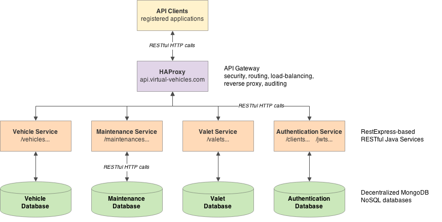
Note: All code available on GitHub. For the version of the code that matches the details in this blog post, check out the master branch, v1.0.0 tag (after running git clone …, run a git checkout tags/v1.0.0 command).
Previous Posts
In Part One of this series, we introduced the microservices-based Virtual-Vehicles REST API example. The vehicle-themed Virtual-Vehicles microservices offers a comprehensive set of functionality, through a REST API, to application developers. In Part Two, we installed a copy of the Virtual-Vehicles project from GitHub. In Part Two, we also gained a basic understanding of how RestExpress works. Finally, we discovered how to get the Virtual-Vehicles microservices up and running.
Part Three
In part three of this series, we will take the Virtual-Vehicles for a test drive (get it? maybe it was funnier the first time…). There are several tools we can use to test the Virtual-Vehicles API. One of my favorite tools is Postman. We will explore how to use Postman, along with the Virtual-Vehicles API documentation, to test the Virtual-Vehicles microservice’s endpoints, which compose the Virtual-Vehicles API.
Testing the API
There are three categories of tools available to test RESTful APIs, which are GUI-based applications, command line tools, and testing frameworks. Postman, Advanced REST Client, REST Console, and SmartBear’s SoapUI and SoapUI NG Pro, are examples of GUI-based applications, designed specifically to test RESTful APIs. cURL and GNU Wget are two examples of command line tools, which among other capabilities, can test APIs. Lastly, JUnit is an example of a testing framework that can be used to test a RESTful API. Surprisingly, JUnit is not only designed to manage unit tests. Each category of testing tools has their pros and cons, depending on your testing needs. We will explore all of these categories in this post as we test the Virtual-Vehicles REST API.
JUnit
JUnit is probably the best known of all Java unit testing frameworks. JUnit’s website describes JUnit as ‘a simple, open source framework to write and run repeatable tests. It is an instance of the xUnit architecture for unit testing frameworks.’ Most Java developers turn to JUnit for unit testing. However, JUnit is capable of other forms of testing, including integration testing. In his post, ‘Unit Testing with JUnit – Tutorial’, Lars Vogel states ‘an integration test has the target to test the behavior of a component or the integration between a set of components. The term functional test is sometimes used as a synonym for integration test. This kind of tests allow you to translate your user stories into a test suite, i.e., the test would resemble an expected user interaction with the application.’
Testing the Virtual-Vehicles RESTful API’s operations with JUnit would be considered integration (functional) testing. At a minimum, to complete requests, we call one microservice, which in turn authenticates the JWT by calling another microservice. If authenticated, the first microservice makes a request to its MongoDB database. As Vogel stated, whereas a unit test targets a small unit of code, such as a method, the request/response operation is integration between a set of components. testing an API call requires several dependencies.
The simplest example of testing the Virtual-Vehicles API with JUnit, would be to test an HTTP GET request to return a single instance of a vehicle. The code below demonstrates how this might be done. Notice the request depends on helper methods (not included, for brevity). To request the vehicle, assuming we already have a registered client, we need a valid JWT. We also need a valid vehicle ObjectId. To obtain these two pieces of data, we call helper methods, which in turn makes the necessary request to retrieve a JWT and vehicle ObjectId.
| /** | |
| * Test of HTTP GET to read a single vehicle. | |
| */ | |
| @Test | |
| public void testVehicleRead() { | |
| String responseBody = ""; | |
| String output; | |
| Boolean result = true; | |
| Boolean expResult = true; | |
| try { | |
| URL url = new URL(getBaseUrlAndPort() + "/vehicles/" + getVehicleObjectId()); | |
| HttpURLConnection conn = (HttpURLConnection) url.openConnection(); | |
| conn.setRequestMethod("GET"); | |
| conn.setRequestProperty("Authorization", "Bearer " + getJwt()); | |
| conn.setRequestProperty("Accept", "application/json"); | |
| if (conn.getResponseCode() != 200) { | |
| // if not 200 response code then fail test | |
| result = false; | |
| } | |
| BufferedReader br = new BufferedReader(new InputStreamReader( | |
| (conn.getInputStream()))); | |
| while ((output = br.readLine()) != null) { | |
| responseBody = output; | |
| } | |
| if (responseBody.length() < 1) { | |
| // if response body is empty then fail test | |
| result = false; | |
| } | |
| conn.disconnect(); | |
| } catch (IOException e) { | |
| // if MalformedURLException, ConnectException, etc. then fail test | |
| result = false; | |
| } | |
| assertEquals(expResult, result); | |
| } |
Below are the results of the above test, run in NetBeans IDE, using the built-in support for JUnit.

JUnit can also be run from the command line using the Maven goal, surefire:test:
| mvn -q -Dtest=com.example.vehicle.objectid.VehicleControllerIT surefire:test |

cURL
One of the best-known command line tools for calling for all types of operations centered around calling a URL is cURL. According to their website, ‘curl is a command line tool and library for transferring data with URL syntax, supporting…HTTP, HTTPS…curl supports SSL certificates, HTTP POST, HTTP PUT, FTP uploading, HTTP form based upload, proxies, HTTP/2, cookies, user+password authentication (Basic, Plain, Digest, CRAM-MD5, NTLM, Negotiate, and Kerberos), file transfer resume, proxy tunneling and more.’ I prefer the website’s briefer description, cURL ‘groks those URLs’.
Using cURL, we could make an HTTP PUT request to the Vehicle microservice’s /vehicles/{oid}.{format} endpoint. With cURL, we have the ability to add the JWT-based Authorization header and the raw request body, containing the modified vehicle object. Below is an example of that cURL command, which can be run from a terminal prompt.
| curl --url 'http://virtual-vehicles.com:8581/vehicles/557310cfec7291b25cd3a1c2' \ | |
| -X PUT \ | |
| -H 'Pragma: no-cache' \ | |
| -H 'Cache-Control: no-cache' \ | |
| -H 'Accept: application/json; charset=UTF-8' \ | |
| -H 'Authorization: Bearer eyJ0eXAiOiJKV1QiLCJhbGciOiJIUzI1NiJ9.eyJpc3MiOiJ2aXJ0dWFsLXZlaGljbGVzLmNvbSIsImFwaUtleSI6IlJncjg0YzF6VkdtMFd1N25kWjd5UGNURSIsImV4cCI6MTQzMzY2ODEwNywiYWl0IjoxNDMzNjMyMTA3fQ.xglaKWufcj4TZtMXW3DLa9uy5JB_FJHxxtk_iF1WT6U' \ | |
| --data-binary $'{ "year": 2015, "make": "Chevrolet", "model": "Corvette Stingray", "color": "White", "type": "Coupe", "mileage": 902, "createdAt": "2015-05-09T22:36:04.808Z" }' \ | |
| --compressed |
The response body contains the expected modified vehicle object in JSON-format, along with a 201 Created response status.

The cURL commands may be incorporated into many types of automated testing processes. These might be as simple as a bash script. The script could a series of automated tests, including the following: register an API client, use the API key to create a JWT, use the JWT to create a new vehicle, use the new vehicle’s ObjectId to modify that same vehicle, delete that vehicle, confirm the vehicle is removed using the count operation and returns a test results report to the user.
cURL Commands from Chrome
Quick tip, instead of hand-coding complex cURL commands, containing form data, URL parameters, and Headers, use Chrome. First, open the Chrome Developer Tools (f12). Next, using the Postman – REST Client for Chrome, available in the Chrome App Store, execute your HTTP request. Finally, in the ‘Network’ tab of the Developers tools, find and right-click on the request and select ‘Copy as cURL’. You have a complete cURL command equivalent of your Postman request, which you can paste directly into the command line or insert into a script. Below is an example of using the Postman – REST Client for Chrome to generate a cURL command.

| curl --url 'http://virtual-vehicles.com:8581/vehicles/554e8bd4c830093007d8b949' \ | |
| -X PUT \ | |
| -H 'Pragma: no-cache' \ | |
| -H 'Origin: chrome-extension://fdmmgilgnpjigdojojpjoooidkmcomcm' \ | |
| -H 'Accept-Encoding: gzip, deflate, sdch' \ | |
| -H 'Accept-Language: en-US,en;q=0.8' \ | |
| -H 'CSP: active' \ | |
| -H 'Authorization: Bearer eyJ0eXAiOiJKV1QiLCJhbGciOiJIUzI1NiJ9.eyJpc3MiOiJ2aXJ0dWFsLXZlaGljbGVzLmNvbSIsImFwaUtleSI6IlBUMklPSWRaRzZoU0VEZGR1c2h6U04xRyIsImV4cCI6MTQzMzU2MDg5NiwiYWl0IjoxNDMzNTI0ODk2fQ.4q6EMuxE0vS43zILjE6e1tYrb5ulCe69-1QTFLYGbFU' \ | |
| -H 'Content-Type: text/plain;charset=UTF-8' \ | |
| -H 'Accept: */*' \ | |
| -H 'User-Agent: Mozilla/5.0 (X11; Linux x86_64) AppleWebKit/537.36 (KHTML, like Gecko) Chrome/43.0.2357.81 Safari/537.36' \ | |
| -H 'Cache-Control: no-cache' \ | |
| -H 'Connection: keep-alive' \ | |
| -H 'X-FirePHP-Version: 0.0.6' \ | |
| --data-binary $'{ "year": 2015, "make": "Chevrolet", "model": "Corvette Stingray", "color": "White", "type": "Coupe", "mileage": 902, "createdAt": "2015-05-09T22:36:04.808Z" }' \ | |
| --compressed |
The generated command is a bit verbose. Compare this command to the cURL command, earlier.
Wget
Similar to cURL, GNU Wget provides the ability to call the Virtual-Vehicles API’s endpoints. According to their website, ‘GNU Wget is a free software package for retrieving files using HTTP, HTTPS and FTP, the most widely-used Internet protocols. It is a non-interactive command line tool, so it may easily be called from scripts, cron jobs, terminals without X-Windows support, etc.’ Again, like cURL, we can run Wget commands from the command line or incorporate them into scripted testing processes. The Wget website contains excellent documentation.
Using Wget, we could make the same HTTP PUT request to the Vehicle microservice /vehicles/{oid}.{format} endpoint. Like cURL, we have the ability to add the JWT-based Authorization header and the raw request body, containing the modified vehicle object.
| wget -O - 'http://virtual-vehicles.com:8581/vehicles/557310cfec7291b25cd3a1c2' \ | |
| --method=PUT \ | |
| --header='Authorization: Bearer eyJ0eXAiOiJKV1QiLCJhbGciOiJIUzI1NiJ9.eyJpc3MiOiJ2aXJ0dWFsLXZlaGljbGVzLmNvbSIsImFwaUtleSI6IlJncjg0YzF6VkdtMFd1N25kWjd5UGNURSIsImV4cCI6MTQzMzY2ODEwNywiYWl0IjoxNDMzNjMyMTA3fQ.xglaKWufcj4TZtMXW3DLa9uy5JB_FJHxxtk_iF1WT6U' \ | |
| --header='Content-Type: text/plain;charset=UTF-8' \ | |
| --header='Accept: application/json' \ | |
| --body-data=$'{ "year": 2015, "make": "Chevrolet", "model": "Corvette Stingray", "color": "White", "type": "Coupe", "mileage": 902, "createdAt": "2015-05-09T22:36:04.808Z" }' |
The response body contains the expected modified vehicle object in JSON-format, along with a 201 Created response status.

cURL Bash Testing
We can combine cURL and Wget with several of the tools bash provides, to develop fairly complex integration tests. The bash-based script below just scratches the surface as a complete set of integration tests. However, the tests demonstrate an efficient multi-stage test approach to handling the complex nature of RESTful service request requirements. The tests build upon each other.
After setting up some variables and doing a quick health check on one service, the tests register a new API client by calling the Authentication service. Next, they use the new client’s API key to obtain a JWT. The tests then use the JWT to authenticate themselves and create a new vehicle. Finally, they use the new vehicle’s id and the JWT to verify the existence for the new vehicle.
Although some may consider using bash to test somewhat primitive, the following script demonstrates the effectiveness of bash’s curl, grep, sed, awk, along with regular expressions, to test our RESTful services. Note how we grep certain values from the response, such as the new client’s API key, and then use that value as a parameter for the following test request, such as to obtain a JWT.
| #!/bin/sh | |
| ######################################################################## | |
| # | |
| # title: Virtual-Vehicles Project Integration Tests | |
| # author: Gary A. Stafford (https://programmaticponderings.com) | |
| # url: https://github.com/garystafford/virtual-vehicles-docker | |
| # description: Performs integration tests on the Virtual-Vehicles | |
| # microservices | |
| # to run: sh tests_color.sh -v | |
| # | |
| ######################################################################## | |
| echo --- Integration Tests --- | |
| ### VARIABLES ### | |
| hostname="localhost" | |
| application="Test API Client $(date +%s)" # randomized | |
| secret="$(date +%s | sha256sum | base64 | head -c 15)" # randomized | |
| echo hostname: ${hostname} | |
| echo application: ${application} | |
| echo secret: ${secret} | |
| ### TESTS ### | |
| echo "TEST: GET request should return 'true' in the response body" | |
| url="http://${hostname}:8581/vehicles/utils/ping.json" | |
| echo ${url} | |
| curl -X GET -H 'Accept: application/json; charset=UTF-8' \ | |
| --url "${url}" \ | |
| | grep true > /dev/null | |
| [ "$?" -ne 0 ] && echo "RESULT: fail" && exit 1 | |
| echo "RESULT: pass" | |
| echo "TEST: POST request should return a new client in the response body with an 'id'" | |
| url="http://${hostname}:8587/clients" | |
| echo ${url} | |
| curl -X POST -H "Cache-Control: no-cache" -d "{ | |
| \"application\": \"${application}\", | |
| \"secret\": \"${secret}\" | |
| }" --url "${url}" \ | |
| | grep '"id":"[a-zA-Z0-9]\{24\}"' > /dev/null | |
| [ "$?" -ne 0 ] && echo "RESULT: fail" && exit 1 | |
| echo "RESULT: pass" | |
| echo "SETUP: Get the new client's apiKey for next test" | |
| url="http://${hostname}:8587/clients" | |
| echo ${url} | |
| apiKey=$(curl -X POST -H "Cache-Control: no-cache" -d "{ | |
| \"application\": \"${application}\", | |
| \"secret\": \"${secret}\" | |
| }" --url "${url}" \ | |
| | grep -o '"apiKey":"[a-zA-Z0-9]\{24\}"' \ | |
| | grep -o '[a-zA-Z0-9]\{24\}' \ | |
| | sed -e 's/^"//' -e 's/"$//') | |
| echo apiKey: ${apiKey} | |
| echo | |
| echo "TEST: GET request should return a new jwt in the response body" | |
| url="http://${hostname}:8587/jwts?apiKey=${apiKey}&secret=${secret}" | |
| echo ${url} | |
| curl -X GET -H "Cache-Control: no-cache" \ | |
| --url "${url}" \ | |
| | grep '[a-zA-Z0-9_-]\{1,\}\.[a-zA-Z0-9_-]\{1,\}\.[a-zA-Z0-9_-]\{1,\}' > /dev/null | |
| [ "$?" -ne 0 ] && echo "RESULT: fail" && exit 1 | |
| echo "RESULT: pass" | |
| echo "SETUP: Get a new jwt using the new client for the next test" | |
| url="http://${hostname}:8587/jwts?apiKey=${apiKey}&secret=${secret}" | |
| echo ${url} | |
| jwt=$(curl -X GET -H "Cache-Control: no-cache" \ | |
| --url "${url}" \ | |
| | grep '[a-zA-Z0-9_-]\{1,\}\.[a-zA-Z0-9_-]\{1,\}\.[a-zA-Z0-9_-]\{1,\}' \ | |
| | sed -e 's/^"//' -e 's/"$//') | |
| echo jwt: ${jwt} | |
| echo "TEST: POST request should return a new vehicle in the response body with an 'id'" | |
| url="http://${hostname}:8581/vehicles" | |
| echo ${url} | |
| curl -X POST -H "Cache-Control: no-cache" \ | |
| -H "Authorization: Bearer ${jwt}" \ | |
| -d '{ | |
| "year": 2015, | |
| "make": "Test", | |
| "model": "Foo", | |
| "color": "White", | |
| "type": "Sedan", | |
| "mileage": 250 | |
| }' --url "${url}" \ | |
| | grep '"id":"[a-zA-Z0-9]\{24\}"' > /dev/null | |
| [ "$?" -ne 0 ] && echo "RESULT: fail" && exit 1 | |
| echo "RESULT: pass" | |
| echo "SETUP: Get id from new vehicle for the next test" | |
| url="http://${hostname}:8581/vehicles?filter=make::Test|model::Foo&limit=1" | |
| echo ${url} | |
| id=$(curl -X GET -H "Cache-Control: no-cache" \ | |
| -H "Authorization: Bearer ${jwt}" \ | |
| --url "${url}" \ | |
| | grep '"id":"[a-zA-Z0-9]\{24\}"' \ | |
| | grep -o '[a-zA-Z0-9]\{24\}' \ | |
| | tail -1 \ | |
| | sed -e 's/^"//' -e 's/"$//') | |
| echo vehicle id: ${id} | |
| echo "TEST: GET request should return a vehicle in the response body with the requested 'id'" | |
| url="http://${hostname}:8581/vehicles/${id}" | |
| echo ${url} | |
| curl -X GET -H "Cache-Control: no-cache" \ | |
| -H "Authorization: Bearer ${jwt}" \ | |
| --url "${url}" \ | |
| | grep '"id":"[a-zA-Z0-9]\{24\}"' > /dev/null | |
| [ "$?" -ne 0 ] && echo "RESULT: fail" && exit 1 | |
| echo "RESULT: pass" |
Since these tests are just a bash script, they can from the command line, or easily called from a continuous integration tool, Such as Jenkins CI or Hudson.
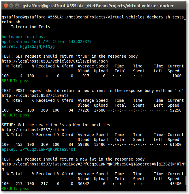
Postman
Postman, like several similar tools, is an application designed specifically for test API endpoints. The Postman website describes Postman as tool that allows you to ‘build, test, and document your APIs faster.’ There are two versions of Postman in the Chrome Web Store. They are Postman – REST Client, the in-browser extension, which we mentioned above, and Postman, the standalone application. There is also Postman Interceptor, which helps you send requests that use browser cookies through the Postman application.
Postman and similar applications, have add-ons and extensions to extend their features. In particular, Postman, which is free, offers the Jetpacks paid extension. Jetpacks add the ability to ‘write and run tests inside Postman, extract data from responses, chain requests together and test requests with thousands of variations’. Jetpacks allow you to move beyond basic one-off API request-based testing, to automated regression and performance testing.
Using Postman
Let’s use the same HTTP PUT example we used with cURL and Wget, and see how we would perform the same task with Postman. In the first screen grab below, you can see all elements of the HTTP request, including the RESTful API’s URL, URI including the vehicle’s ObjectId (/vehicles/{ObjectId}.{format}), HTTP method (PUT), Authorization Header with JWT (Bearer), and the raw request body. The raw request body contains a JSON representation of the vehicle we want to update. Note how Postman saves the request in history so we can easily replay it later.

In the next screen-grab, we see the response to the HTTP PUT request. Note the response body, response status, timing, and response headers.

Looking at the response body in Postman, you easily see the how RestExpress demonstrates the RESTful principle we discussed in Part Two of the series, HATEOAS (Hypermedia as the Engine of Application State). Note the link to this vehicle’s ‘self’ href) and the entire vehicles collection (‘up’ href).
Postman Collections
A great feature of Postman with Jetpacks is Collections. Collections are sets of requests, which can be saved, recalled, and shared. The Collection Runner runs requests in a collection, in the order in which you set them. Ordered collections are ideal for the Virtual-Vehicles API. The screen grab below shows a collection of requests, arranged in the order we would execute them to test the Virtual-Vehicles API, as it applies to specifically to vehicle CRUD operations:
- Execute HTTP POST request to register the new API client, passing the application name and a shared secret in the request
Receive the new client’s API key in response - Execute HTTP GET to request, passing the new client’s API key and the shared secret in the request
Receive the new JWT in response - Execute HTTP POST request to create a new vehicle, passing the JWT in the header for authentication (used for all following requests)
Receive the new vehicle object in response - Execute HTTP PUT request to modify the new vehicle, using the vehicle’s
ObjectId
Receive the modified vehicle object in response - Execute HTTP GET to request the modified vehicle, to confirm it exists in the expected state
Receive the vehicle object in response - Execute HTTP DELETE request to delete the new vehicle, using the vehicle’s
ObjectId - Execute HTTP GET to request the new vehicle and to confirm it has been removed
Receive a 404 Not Found status response, as expected

Using saved collections for testing the Virtual-Vehicles API is a real-time saving. However, the collections cannot easily be re-run without hand-editing or some advanced scripting. In the simple example above, we hard-coded a JWT and vehicle ObjectId in the requests. Unfortunately, the JWT has an expiration of only 10 hours by default. More immediately, the ObjectId is unique. The earlier collection test run created, then deleted, the vehicle with that ObjectId.
Negative Testing
You may also perform negative testing with Postman. For example, do you receive the expected response when you don’t include the Authorization Header with JWT in a request (401 Unauthorized status)? When you include a JWT, which has expired (401 Unauthorized status)? When you request a vehicle, whose ObjectId is incorrect or is not found in the database (400 Bad Request status)? Do you receive the expected response when you call an actual service, but an endpoint that doesn’t exist (405 Method Not Allowed)?

Postman Test Automation
In addition to manually viewing the HTTP response, to verify the results of a request, Postman allows you to write and run automated tests for each request. According to their website, a ‘Postman test is essentially JavaScript code which sets values for the special tests object. You can set a descriptive key for an element in the object and then say if it’s true or false’. This allows you to write a set of response validation tests for each request.
Below is a quick example of testing the same HTTP POST request, used to create the new API client, above. In this example, we:
- Test that the
Content-Typeresponse header is present - Test that the HTTP POST successfully returned a 201 status code
- Test that the new client’s API key was returned in the response body
- Test that the response time was less than 200ms

Reviewing Postman’s ‘Tests’ tab, above, observe the four tests have run successfully. Using the Postman’s testing feature, you can create even more advanced tests, eliminating the need to manually validate responses.
This post demonstrates a small subset of the features Postman and other similar applications provide for testing RESTful API. The tools and processes you use to test your RESTful API will depend on the stage of development and testing you are in, as well as the existing technology stacks you build, and on which you host your services.
Building a Microservices-based REST API with RestExpress, Java EE, and MongoDB: Part 2
Posted by Gary A. Stafford in Enterprise Software Development, Java Development, Software Development on May 31, 2015
Develop a well-architected and well-documented REST API, built on a tightly integrated collection of Java EE-based microservices.
Note: All code available on GitHub. For the version of the code that matches the details in this blog post, check out the master branch, v1.0.0 tag (after running git clone …, run a ‘git checkout tags/v1.0.0’ command).
Previous Post
In Part One of this series, we introduced the microservices-based Virtual-Vehicles REST API example. The vehicle-themed Virtual-Vehicles microservices offers a comprehensive set of functionality, through a REST API, to application developers. The developers, in turn, will use the Virtual-Vehicles REST API’s functionality to build applications and games for their end-users.
In Part One, we also decided on the proper amount and responsibility of each microservice. We also determined the functionality of each microservice to meet the hypothetical functional and nonfunctional requirements of Virtual-Vehicles. To review, the four microservices we are building, are as follows:
Virtual-Vehicles REST API Resources |
||
| Microservice | Purpose (Business Capability) | Functions |
| Authentication |
Manage API clients and JWT authentication |
|
| Vehicle |
Manage virtual vehicles |
|
| Maintenance |
Manage maintenance on vehicles |
|
| Valet Parking |
Manage a valet service to park for vehicles |
|
To review, the first five functions for each service are all basic CRUD operations: create (POST), read (GET), readAll (GET), update (PUT), delete (DELETE). The readAll function also has find, count, and pagination functionality using query parameters. Unfortunately, RestExpress does not support PATCH for updates. However, I have updated RestExpress’ PUT HTTP methods to return the modified object in the response body instead of the nothing (status of 201 Created vs. 200 OK). See StackOverflow for an explanation.
All services also have an internal authenticateJwt function, to authenticate the JWT, passed in the HTTP request header, before performing any operation. Additionally, all services have a basic health-check function, ping (GET). There are only a few other functions required for our Virtual-Vehicles example, such as for creating JWTs.
Part Two Introduction
In Part Two, we will build our four Virtual-Vehicles microservices. Recall from our first post, we will be using RestExpress. RestExpress composes best-of-breed open-source tools to enable quickly creating RESTful microservices that embrace industry best practices. Those best-of-breed tools include Java EE, Maven, MongoDB, and Netty, among others.
In this post, we will accomplish the following:
- Create a default microservice project in NetBeans using RestExpress MongoDB Maven Archetype
- Understand the basic structure of a default RestExpress microservice project
- Review the changes made to the default RestExpress microservice project to create the Virtual-Vehicles example
- Compile and run the individual microservices directly from NetBeans
I used NetBeans IDE 8.0.2 on Linux Ubuntu 14.10 to build the microservices. You may also follow along in other IDE’s, such as Eclipse or IntelliJ, on Mac or Windows. We won’t cover installing MongoDB, Maven, and Java. I’ll assume if your building enterprise applications, you have the basics covered.
Using the RestExpress MongoDB Maven Archetype
All the code for this project is available on GitHub. However, to understand RestExpress, you should go through the exercise of scaffolding a new microservice using the RestExpress MongoDB Maven Archetype. You will also be able to use this default microservice project to compare and contrast to the modified versions, used in the Virtual-Vehicles example. The screen grabs below demonstrate how to create a new microservice project using the RestExpress MongoDB Maven Archetype. At the time of this post, the archetype version was restexpress-mongodb version 1.15.


Default Project Architecture
Reviewing the two screen grabs below (Project tab), note the key components of the RestExpress MongoDB Maven project, which we just created:
- Base Package (com.example.vehicle)
- Configuration class reads in environment properties (see Files tab) and instantiates controllers
- Constants class contains project constants
- Relationships class defines linking resource which aids service discoverability (HATEOAS)
- Main executable class
- Routes class defines the routes (endpoints) exposed by the service and the corresponding controller class
- Model/Controllers Packages (com.example.vehicle.objectid and .uuid)
- Entity class defines the data entity – a Vehicle in this case
- Controller class contains the methods executed when the route (endpoint) is called
- Repository class defines the connection details to MongoDB
- Service class contains the calls to the persistence layer, validation, and business logic
- Serialization Package (com.example.vehicle.serialization)
- XML and JSON serialization classes
- Object ID and UUID serialization and deserialization classes


Again, I strongly recommend reviewing each of these package’s classes. To understand the core functionality of RestExpress, you must understand the relationships between RestExpress microservice’s Route, Controller, Service, Repository, Relationships, and Entity classes. In addition to reviewing the default Maven project, there are limited materials available on the Internet. I would recommend the RestExpress Website on GitHub, RestExpress Google Group Forum, and the YouTube 3-part video series, Instant REST Services with RESTExpress.
Unit Tests?
Disappointingly, the current RestExpress MongoDB Maven Archetype sample project does not come with sample JUnit unit tests. I am tempted to start writing my own unit tests if I decided to continue to use the RestExpress microservices framework for future projects.
Properties Files
Also included in the default RestExpress MongoDB Maven project is a Java properties file (environment.properties). This properties file is displayed in the Files tab, as shown below. The default properties file is located in the ‘dev’ environment config folder. Later, we will create an additional properties file for our production environment.

Ports
Within the ‘dev’ environment, each microservice is configured to start on separate ports (i.e. port = 8581). Feel free to change the service’s port mappings if they conflict with previously configured components running on your system. Be careful when changing the Authentication service’s port, 8587, since this port is also mapped in all other microservices using the authentication.port property (authentication.port = 8587). Make sure you change both properties, if you change Authentication service’s port mapping.
Base URL
Also, in the properties files is the base.url property. This property defines the URL the microservice’s endpoints will be expecting calls from, and making internal calls between services. In our post’s example, this property in the ‘dev’ environment is set to localhost (base.url = http://localhost). You could map an alternate hostname from your hosts file (/etc/hosts). We will do this in a later post, in our ‘prod’ environment, mapping the base.url property to Virtual-Vehicles (base.url = http://virtual-vehicles.com). In the ‘dev’ environment properties file, MongoDB is also mapped to localhost (i.e. mongodb.uri = mongodb://virtual-vehicles.com:27017/virtual_vehicle).
Metrics Plugin and Graphite
RestExpress also uses the properties file to hold configuration properties for Metrics Plugin and Graphite. The Metrics Plugin and Graphite are both first class citizens of RestExpress. Below is the copy of the Vehicles service environment.properties file for the ‘dev’ environment. Note, the Metrics Plugin and Graphite are both disabled in the ‘dev’ environment.
| # Default is 8081 | |
| port = 8581 | |
| # Port used to call Authentication service endpoints | |
| authentication.port = 8587 | |
| # The size of the executor thread pool | |
| # (that can handle blocking back-end processing). | |
| executor.threadPool.size = 20 | |
| # A MongoDB URI/Connection string | |
| # see: http://docs.mongodb.org/manual/reference/connection-string/ | |
| mongodb.uri = mongodb://localhost:27017/virtual_vehicle | |
| # The base URL, used as a prefix for links returned in data | |
| base.url = http://localhost | |
| #Configuration for the MetricsPlugin/Graphite | |
| metrics.isEnabled = false | |
| #metrics.machineName = | |
| metrics.prefix = web1.example.com | |
| metrics.graphite.isEnabled = false | |
| metrics.graphite.host = graphite.example.com | |
| metrics.graphite.port = 2003 | |
| metrics.graphite.publishSeconds = 60 |
Choosing a Data Identification Method
RestExpress offers two identification models for managing data, the MongoDB ObjectId and a Universally Unique Identifier (UUID). MongoDB uses an ObjectId to identify uniquely a document within a collection. The ObjectId is a special 12-byte BSON type that guarantees uniqueness of the document within the collection. Alternately, you can use the UUID identification model. The UUID identification model in RestExpress uses a UUID, instead of a MongoDB ObjectId. The UUID also contains createdAt and updatedAt properties that are automatically maintained by the persistence layer. You may stick with ObjectId, as we will in the Virtual-Vehicles example, or choose the UUID. If you use multiple database engines for your projects, using UUID will give you a universal identification method.
Project Modifications
Many small code changes differentiate our Virtual-Vehicles microservices from the default RestExpress Maven Archetype project. Most changes are superficial; nothing changed about how RestExpress functions. Changes between the screen grabs above, showing the default project, and the screen grabs below, showing the final Virtual-Vehicles microservices, include:
- Remove all packages, classes, and code references to the UUID identification methods (example uses ObjectId)
- Rename several classes for convenience (dropped use of word ‘Entity’)
- Add the Utilities (com.example.utilities) and Authentication (com.example.authenticate) packages


MongoDB
Following a key principle of microservices mentioned in the first post, Decentralized Data Management, each microservice will have its own instance of a MongoDB database associated with it. The below diagram shows each service and its corresponding database, collection, and fields.

From the MongoDB shell, we can observe the individual instances of the four microservice’s databases.

In the case of the Vehicle microservice, the associated MongoDB database is virtual_vehicle. This database contains a single collection, vehicles. While the properties file defines the database name, the Vehicles entity class defines the collection name, using the org.mongodb.morphia.annotations classes annotation functionality.
| @Entity("vehicles") | |
| public class Vehicle | |
| extends AbstractMongodbEntity | |
| implements Linkable { | |
| private int year; | |
| private String make; | |
| private String model; | |
| private String color; | |
| private String type; | |
| private int mileage; | |
| // abridged... |
Looking at the virtual_vehicle database in the MongoDB shell, we see that the sample document’s fields correspond to the Vehicle entity classes properties.

Each of the microservice’s MongoDB databases are configured in the environments.properties file, using the mongodb.uri property. In the ‘dev’ environment we use localhost as our host URL (i.e. mongodb.uri = mongodb://localhost:27017/virtual_vehicle).
Authentication and JSON Web Tokens
The three microservices, Vehicle, Valet, and Maintenance, are almost identical. However, the Authentication microservice is unique. This service is called by each of the other three services, as well as also being called directly. The Authentication service provides a very basic level of authentication using JSON Web Tokens (JWT), pronounced ‘jot‘.
Why do we want authentication? We want to confirm that the requester using the Virtual-Vehicles REST API is the actual registered API client they are who they claim to be. JWT allows us to achieve this requirement with minimal effort.
According to jwt.io, ‘a JSON Web Token is a compact URL-safe means of representing claims to be transferred between two parties. The claims in a JWT are encoded as a JSON object that is digitally signed using JSON Web Signature (JWS).‘ I recommend reviewing the JWT draft standard to fully understand the structure, creation, and use of JWTs.
Virtual-Vehicles Authentication Process
There are different approaches to implementing JWT. In our Virtual-Vehicles REST API example, we use the following process for JWT authentication:
- Register the new API client by supplying the application name and a shared secret (one time only)
- Receive an API key in response (one time only)
- Obtain a JWT using the API key and the shared secret (each user session or renew when the previous JWT expires)
- Include the JWT in each API call
In our example, we are passing four JSON fields in our set of claims. Those fields are the issuer (‘iss’), API key, expiration (‘exp’), and the time the JWT was issued (‘ait’). Both the ‘iss’ and the ‘exp’ claims are defined in the Authentication service’s environment.properties file (jwt.expire.length and jwt.issuer).
Expiration and Issued date/time use the JWT standard recommended “Seconds Since the Epoch“. The default expiration for a Virtual-Vehicles JWT is set to an arbitrary 10 hours from the time the JWT was issued (jwt.expire.length = 36000). That amount, 36,000, is equivalent to 10 hours x 60 minutes/hour x 60 seconds/minute.
Decoding a JWT
Using the jwt.io site’s JT Debugger tool, I have decoded a sample JWT issued by the Virtual-Vehicles REST API, generated by the Authentication service. Observe the three parts of the JWT, the JOSE Header, Claims Set, and the JSON Web Signature (JWS).

The JWT’s header indicates that our JWT is a JWS that is MACed using the HMAC SHA-256 algorithm. The shared secret, passed by the API client, represents the HMAC secret cryptographic key. The secret is used in combination with the cryptographic hash function to calculate the message authentication code (MAC). In the example below, note how the API client’s shared secret is used to validate our JWT’s JWS.
Sequence Diagrams of Authentication Process
Below are three sequence diagrams, which detail the following processes: API client registration process, obtaining a new JWT, and a REST call being authenticated using the JWT. The end-user of the API self-registers their application using the Authentication service and receives back an API key. The API key is unique to that client.
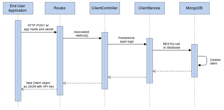
The end-user application then uses the API key and the shared secret to receive a JWT from the Authentication service.
 After receiving the JWT, the end-user application passes the JWT in the header of each API request. The JWT is validated by calling the Authentication service. If the JWT is valid, the request is fulfilled. If not valid, a ‘401 Unauthorized’ status is returned.
 JWT Validation
The JWT draft standard recommends how to validate a JWT. Our Virtual-Vehicles Authentication microservice uses many of those criteria to validate the JWT, which include:
- API Key – Retrieve API client’s shared secret from MongoDB, using API key contained in JWT’s claims set (secret is returned; therefore API key is valid)
- Algorithm – confirm the algorithm (‘alg’), found in the JWT Header, which used to encode JWT, was ‘HS256’ (HMAC SHA-256)
- Valid JWS – Use the client’s shared secret from #1 above, decode HMAC SHA-256 encrypted JWS
- Expiration – confirm JWT is not expired (‘exp’)
Inter-Service Communications
By default, the RestExpress Archetype project does not offer an example of communications between microservices. Service-to-service communications for microservices is most often done using the same HTTP-based REST calls used to by our Virtual-Vehicles REST API. Alternately, a message broker, such as RabbitMQ, Kafka, ActiveMQ, or Kestrel, is often used. Both methods of communicating between microservices, referred to as ‘inter-service communication mechanisms’ by InfoQ, have their pros and cons. The InfoQ website has an excellent microservices post, which discusses the topic of service-to-service communication.
For the Virtual-Vehicles microservices example, we will use HTTP-based REST calls for inter-service communications. The primary service-to-service communications in our example, is between the three microservices, Vehicle, Valet, and Maintenance, and the Authentication microservice. The three services validate the JWT passed in each request to a CRUD operation, by calling the Authentication service and passing the JWT, as shown in the sequence diagram, above. Validation is done using an HTTP GET request to the Authentication service’s .../jwts/{jwt} endpoint. The Authentication service’s method, called by this endpoint, minus some logging and error handling, looks like the following:
| public boolean authenticateJwt(Request request, String baseUrlAndAuthPort) { | |
| String jwt, output, valid = ""; | |
| try { | |
| jwt = (request.getHeader("Authorization").split(" "))[1]; | |
| } catch (NullPointerException | ArrayIndexOutOfBoundsException e) { | |
| return false; | |
| } | |
| try { | |
| URL url = new URL(baseUrlAndAuthPort + "/jwts/" + jwt); | |
| HttpURLConnection conn = (HttpURLConnection) url.openConnection(); | |
| conn.setRequestMethod("GET"); | |
| conn.setRequestProperty("Accept", "application/json"); | |
| if (conn.getResponseCode() != 200) { | |
| return false; | |
| } | |
| BufferedReader br = new BufferedReader(new InputStreamReader( | |
| (conn.getInputStream()))); | |
| while ((output = br.readLine()) != null) { | |
| valid = output; | |
| } | |
| conn.disconnect(); | |
| } catch (IOException e) { | |
| return false; | |
| } | |
| return Boolean.parseBoolean(valid); | |
| } |
Primarily, we are using the java.net and java.io packages, along with the org.restexpress.Request class to build and send our HTTP request to the Authentication service. Alternately, you could use just the org.restexpress package to construct request and handle the response. This same basic method structure shown above can be used to create unit tests for your service’s endpoints.
Health Ping
Each of the Virtual-Vehicles microservices contain a DiagnosticController in the .utilities package. In our example, we have created a ping() method. This simple method, called through the .../utils/ping endpoint, should return a 200 OK status and a boolean value of ‘true’, indicating the microservice is running and reachable. This route’s associated method could not be simpler:
| public void ping(Request request, Response response) { | |
| response.setResponseStatus(HttpResponseStatus.OK); | |
| response.setResponseCode(200); | |
| response.setBody(true); | |
| } |
The ping health check can even be accessed with a simple curl command, curl localhost:8581/vehicles/utils/ping.
In a real-world application, we would add additional health checks to all services, providing additional insight into the health and performance of each microservice, as well as the service’s dependencies.
API Documentation
A well written RESTful API will not require extensive documentation to understand the API’s operations. Endpoints will be discoverable through linking (see Response Body links section in below example). API documentation should provide HTTP method, required headers and URL parameters, expected response body and response status, and so forth.
An API should be documented before any code is written, similar to TDD. The API documentation is the result of a clear understanding of requirements. The API documentation should make the coding even easier since the documentation serves as a further refinement of the requirements. The requirements are an architectural plan for the microservice’s code structure.
Sample Documentation
Below, is a sample of the Virtual-Vehicles REST API documentation. It details the function responsible for creating a new API client. The documentation provides a brief description of the function, the operation’s endpoint (URI), HTTP method, request parameters, expected response body, expected response status, and even a view of the MongoDB collection’s document for a new API client.

You can download a PDF version of the Virtual-Vehicles RESTful API documentation on GitHub or review the source document on Google Docs. It contains general notes about the API, and details about every one of the API’s operations.
Running the Individual Microservices
For development and testing purposes, the easiest way to start the microservices is in NetBeans using the Run command. The Run command executes the Maven exec goal. Based on the DEFAULT_ENVIRONMENT constant in the org.restexpress.util Environment class, RestExpress will use the ‘dev’ environment’s environment.properties file, in the project’s /config/dev directory.
Alternately, you can use the RestExpress project’s recommended command from a terminal prompt to start each microservice from its root directory (mvn exec:java -Dexec.mainClass=test.Main -Dexec.args="dev"). You can also use this command to switch from the ‘dev’ to ‘prod’ environment properties (-Dexec.args="prod").
You may use a variety of commands to confirm all the microservices are running. I prefer something basic like sudo netstat -tulpn | grep 858[0-9]. This will find all the ports within the ‘dev’ port range. For more in-depth info, you can use a command like ps -aux | grep com.example | grep -v grep

Part Three: Testing our Services
We now have a copy of the Virtual-Vehicles project pulled from GitHub, a basic understanding of how RestExpress works, and our four microservices running on different ports. In Part Three of this series, we will take them for a drive (get it?). There are many ways to test our service’s endpoints. One of my favorite tools is Postman. we will explore how to use several tools, including Postman, and our API documentation, to test our microservice’s endpoints.

Building a Microservices-based REST API with RestExpress, Java EE, and MongoDB: Part 1
Posted by Gary A. Stafford in Enterprise Software Development, Java Development, Software Development on May 18, 2015
Develop a well-architected and well-documented REST API, built on a tightly integrated collection of Java EE-based microservices.
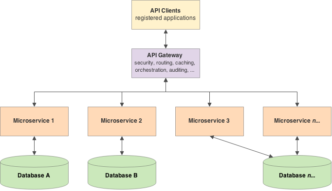
Microservices
Microservices are a popular and growing trend in software development. According to Wikipedia, microservices are “a software architecture style, in which complex applications are composed of small, independent processes communicating with each other using language-agnostic APIs. These services are small, highly decoupled and focus on doing a small task.”
Martin Fowler and James Lewis (ThoughtWorks) have done an exemplary job capturing the essence of microservice architecture in their March 2014 post, microservices. Fowler has also discussed these principles in several presentations, including the January 2015 goto; Conference, Keynote: Microservices by Martin Fowler.
Additionally, noted technical consultant and speaker, Adrian Cockcroft (Battery Ventures), has made significant contributions to the definition of microservices, such as in his December 2014 dockercon14 | eu presentation, State of the Art in Microservices.
Lastly, Zhamak Dehghani (ThoughtWorks), delivered an in-depth discussion of microservices, including customer perspectives, in her October 2014 presentation, Real-World Microservices: Lessons from the Frontline.
Some of the major characteristics of microservices and REST cited by these experts, include:
- Organized Around Business Capabilities
- Single Responsibility
- Loose Coupling / High Cohesion
- Smart Endpoints and Dumb Pipes
- Decentralized Data Management
- Hypermedia as the Engine of Application State (HATEOAS)
As we develop this post’s example, I will demonstrate how all of the above characteristics are implemented.
REST API
A REST API is the mash-up of two common software concepts, Representational State Transfer (REST) and an application programming interface (API). Although even Wikipedia doesn’t have an exact definition of a REST API, they come close to their discussion of REST. According to Wikipedia, “Web service APIs that adhere to the REST architectural constraints are called RESTful APIs. HTTP-based RESTful APIs are defined with these aspects: base URI, an Internet media type for the data, standard HTTP methods, hypertext links to a reference state, and hypertext links to reference related resources.”
An important nuance and differentiator from SOA-based APIs, RESTful APIs do not require XML-based Web service protocols (SOAP and WSDL) to support their interfaces (Wikipedia).
The author of the WebConcepts channel does an excellent job capturing the essence of REST APIs in REST API concepts and examples. Two additional presentations I strongly recommend are REST+JSON API Design – Best Practices for Developers and Designing a Beautiful REST+JSON API, both by Les Hazlewood, CTO of Stormpath. Stormpath is a leader in the commercial REST API space.
Microservices-Based REST API
A microservices-based REST API is a REST API, whose HTTP requests call an orchestrated collection or collections of language-agnostic and platform-agnostic microservices. The combination of these two trends, microservices, and a REST API, offers a simple, reliable, and scalable solution for providing flexible functionality to an end-user, in a technology-agnostic manner.
REST API Example
There is a fast-growing volume of reference materials describing the characteristics, benefits, and general architecture of microservices and REST APIs. However, in researching these topics, I have found a shortage of practical examples or tutorials on building microservices-based REST API solutions.
Undoubtedly, the complexity of even the simplest microservices-based solution limits the number of available cases. A minimally viable solution require planning, coding, testing, and documentation. The addition of cross-cutting features such as security, logging, monitoring, and orchestration, creates an enormous task to build a practical microservices-based example.
In the following series of posts, we will use many of the characteristics of a modern microservice architecture as described by Fowler, Lewis, Cockcroft, and Dehghani. We will combine these microservice characteristics with the best practices of good REST API design, as described by Hazlewood and WebConcepts, to build a minimally viable microservices-based REST API.
In a future post, we will create an application, which leverages the microservices-based solution, through the REST API. Additionally, we will demonstrate how to ensure high-availability of the individual microservices and data sources.
Vehicle for Learning
In a similar vein to the publicly available Twitter, Facebook, and Google REST APIs, we will build the Virtual-Vehicles REST API. The Virtual-Vehicles REST API will constitute a collection of vehicle-themed microservices. Collectively, the microservices will offer a comprehensive set of functionality to the end-user, an application developer. They, in turn, will use the functionality of the Virtual-Vehicles REST API to build applications and games for their end-users.
Technology Choices
There are a seemingly infinite number of technology choices for building microservices and REST APIs. Your choice of development languages, databases, application servers, third-party libraries, API gateway, logging, monitoring, automated testing, ORM or ODM, and even the IDE, all define your technology stack.
For the Virtual-Vehicles solution, we will use the following key technologies:
- RestExpress-Create performant, stand-alone microservices-based REST APIs
- Java EE – Primary development language
- Netty – Async, event-driven Java network application framework
- Apache Maven – Dependency management and more
- MongoDB – Data source
- JSON Web Tokens (JWT) – Claims-based authentication
- Apache Log4j 2 – Logging
- JUnit – Unit testing
- HAProxy – Service gateway and load-balancing
- NetBeans – IDE
- Git and GitHub – SCM
- Postman – REST API testing
What is RestExpress?
According to their website, RestExpress, composes best-of-breed open-source tools to enable quickly creating RESTful microservices that embrace industry best practices. Built from the ground-up for container-less, microservice architectures, RestExpress is the easiest way to create RESTful APIs in Java. RestExpress is an extremely lightweight, fast, REST engine and API for Java. RestExpress is a thin wrapper on Netty IO HTTP handling. RestExpress lets you create performant, stand-alone REST APIs rapidly. RestExpress provides several Maven archetypes, which we will use as a basis for our microservices.
RestExpress will also drive our technology decisions to use Java EE, Maven, MongoDB, and Netty.
Virtual-Vehicles Microservices
Adhering to the first few microservice architectural principles listed above, organized around business capabilities, single responsibility, and high cohesion, we first must determine the proper number of microservices, and their individual responsibilities. In the case of our solution, we will break down Virtual-Vehicles’ business capabilities into the following microservices:
Virtual-Vehicles Services |
|
| Microservice | Purpose (Business Capability) |
| Authentication Service | Manage API clients and JWT authentication |
| Vehicle Service | Manage virtual vehicles |
| Maintenance Service | Manage maintenance on vehicles |
| Valet Parking Service | Manage a valet service to park for vehicles |
| Sales Service | Manage the buying and selling of vehicles |
| Registration Service | Manage registration of vehicles to owners |
| Auction Service | Manage a virtual car auction |
| Car Show Service | Manage a virtual car show |
| Interaction Service | Manage interaction of users with vehicles |
For simplicity in this post’s example, we will only be exploring the (4) services shown above in bold.
This segmentation of service functionality is unlike what we might encounter in traditional monolithic, n-tier applications, and SOA-based architecture. Traditional applications were built around application-centric functionality or business’ organizational structure. Microservices, however, are client-centric and built around business capabilities.
REST API Functionality
The next decision we need to make is required functionality. What are the operational requirements of each business segment, represented by the microservices? Additionally, what are the nonfunctional requirements, such as monitoring, logging, and authentication. Requirements are translated into functionality, which is translated into the available resources exposed via the service’s RESTful endpoints.
For the Virtual-Vehicles microservices solution, based on a hypothetical set of business and non-functional requirements, we will expose the following resources. Collectively, they will compose the REST API:
Virtual-Vehicles REST API Resources |
||
| Microservice | Purpose (Business Capability) | Functions |
| Authentication Service | Manage API clients and JWT authentication |
|
| Vehicle Service | Manage virtual vehicles |
|
| Maintenance Service | Manage maintenance on vehicles |
|
| Valet Parking Service | Manage a valet service to park for vehicles |
|
Reviewing the table above, note the first five functions for each service are all basic CRUD operations: create (POST), read (GET), readAll (GET), update (PUT), delete (DELETE). The readAll function also has find, count, and pagination functionality using query parameters.
All services also have an internal authenticateJwt function, to authenticate the JWT, passed in the HTTP request header, before performing any operation. Additionally, all services have a basic health-check function, ping (GET). There are only a few other functions required for our Virtual-Vehicles example, such as for creating JWTs.
I’ve labeled each function as to suggested user scope. Scopes include public, admin, and internal. As a consumer of the REST API, you may only want to expose certain functionality to your general end-user (public). Additional functionality may be reserved for an administrative user (admin) or only yourself as a developer (internal). Creating a new vehicle might be a common end-user feature. However, the ability to permanently delete one or more vehicles may be reserved for an admin-level user, or not exposed at all.
REST API Patterns
We will not spend a lot of time discussing patterns for building REST APIs. There are many useful materials available on the Internet regarding industry-standard patterns for REST API resource URI construction. The two presentations I recommend above by Les Hazlewood, CTO of Stormpath, are excellent. Also, Microservices.io, RestApiTutorial.com, swagger.io, and raml.org websites offer solid overviews of REST patterns and RESTful standards.
A common RESTful anti-pattern, which is hard to avoid as a OOP developer, is the temptation to use verbs versus nouns and method-like names, in resource URIs. Remember, we are not designing an end-user application. We are building an API, used by API consumers (application developers), to build a variety of platform and language-agnostic applications. Functions like paintCar, changeOil, or parkVehicle are not something the API should define. The Vehicle microservice exposes the update operation, which allows an application developer to change the car’s paint color in their paintCar method. Similarly, the valet service exposes the create operation, which allows the application developer to create a function to park the vehicle (or car, or truck, in a garage, or parking lot, etc.). A good REST API allows for maximum end-user flexibility.
Part Two
In Part Two, we will install a copy of the Virtual-Vehicles project from GitHub. In Part Two, we will gain a basic understanding of how RestExpress works. Finally, we will discover how to get the Virtual-Vehicles microservices up and running.
Instant Oracle Database and PowerShell How-to Book
Posted by Gary A. Stafford in Oracle Database Development, PowerShell Scripting on March 30, 2013
Recently, I finished reading Geoffrey Hudik‘s Instant Oracle Database and PowerShell How-to ebook, part of Packt Publishing‘s Instant book series. Packt’s Instant book series promises short, fast, and focused information; Hudik’s book delivers. It’s eighty pages deliver hundreds of pages worth of the author’s knowledge in a highly-condensed format, perfect for today’s multi-tasking technical professionals.
Hudik’s book is ideal for anyone experienced with the Oracle Database 11g platform, and interested in leveraging Microsoft’s PowerShell scripting technology to automate their day-to-day database tasks. Even a seasoned developer, experienced in both technologies, will gain from the author’s insight on overcoming several PowerShell and .NET framework related integration intricacies.
As a busy developer, I was able to immediately start implementing many of the book’s recipes to improve my productivity. I especially enjoyed the way the book builds upon previous lessons, resulting in a useful collection of foundational PowerShell scripts and modules. Building on top of these, save time when automating a new task.

Getting started with the book’s examples required a few free downloads from Oracle and Microsoft. Starting with a Windows 7 Enterprise laptop, I downloaded and installed Oracle Database 11g Express Edition (Oracle Database XE) Release 2,
Oracle Developer Tools for Visual Studio, and Oracle SQL Developer IDE. I also made sure my laptop was up-to-date with the latest Visual Studio 2012, .NET framework, and PowerShell updates.
If you are new to administering Oracle databases or using Oracle SQL Developer IDE, Oracle has some excellent interactive tutorials online to help you get started.
Database First Development with Entity Framework 5 in Visual Studio 2012
Posted by Gary A. Stafford in .NET Development, Software Development on November 22, 2012
Build and test a Data Access Layer (DAL) using Entity Framework 5 and Database First Development in Visual Studio 2012. Use the Entity Framework Designer to build an ADO.NET Entity Data Model containing database tables, views, stored procedures, and scalar-valued functions. An updated version of this project’s source code, using EF6 is now available on GitHub. The GitHub repository contains all three Entity Framework blog posts.
![]()
Introduction
In the last post, we explored Microsoft’s new Entity Framework 5 with Code First Development. In this post, we will explore Entity Framework 5 with Database First Development. We will be using the same data model as before. However, this time instead of POCOs, we will start with a SQL Server 2008 R2 database and use the Entity Framework Designer to build an ADO.NET Entity Data Model (EDM). In addition to database tables, we will look at Entity Framework’s ability to support database views (virtual tables), stored procedures, and scalar-valued functions.
Download a complete copy of the post’s source code, with SQL scripts to create the database objects and populate the database with sample data, from DropBox.
Entity Framework’s Code First and Model First development offer many great options for .NET developers. However, in my experience, most enterprise-level application developers work with a Database First Development model. Using Database First Development, Entity Framework 5 (EF5) provides the ability to construct a powerful yet easy-to-implement data access layer (DAL) between the database and the business logic.
The steps involved in this example are as follows:
- Create the new SQL Server database;
- Create the database objects;
- Create a new C# Class Library Project in Visual Studio 2012 Solution;
- Add a new ADO.NET Entity Data Model to project;
- Create a new Database Connection;
- Import the database objects into the EDM;
- Modify the EDM to accommodate the scalar-valued functions;
- Populate the database with sample data;
- Validate the EDM using a Unit Test Project;
Below is a final view of the entire Solution for reference as you work through the post.

Solution Explorer View of Final Solution
The Database
Using SQL Server 2008 R2 Management Studio (SSMS), Toad for SQL, or similar application, create a new database, named ‘HealthTracker’. I left all the default database settings unchanged for this post.

Create the New Health Tracker Database
Next, execute the supplied sql script to populate the HealthTracker database with the necessary database objects. The script should insert the following objects: (6) tables, (1) view, (1) stored procedure, (3) scalar-valued functions, and all the necessary table relationships. All objects will be members of the default ‘dbo’ schema.

Database in SQL Server Object Viewer
Barring a few minor changes, this data model is identical to the one we built in the last post using Code First Development with POCOs. The below Database Diagram illustrates the one-to-many relationships between the tables. The tables are pluralized in the database, as opposed to singular in the ADO.NET Entity Data Model (Meals vs. Meal, People vs. Person, etc.). This is a common pattern with Entity Framework.

Database Diagram of Table Relationships
Optional: Setting Up Database Credentials
For security and simplicity, I choose to add a new Login, User, and Role to the database. This step is not necessary for this post. However, it is good to get into the habit of securing your database, using database Logins, Users, Roles, and Permissions. In addition, if you are planning to deploy the database and the DAL to other environments such as Test or Production, don’t tie your Solution to personal credentials, a machine-specific account, or to an administrative role in the database with overly broad permissions.
The Database User, DemoUser, is associated with the Login, DemoLogin. DemoUser is a member of the Database Role, DemoRole. I will use the DemoLogin account to connect the EDM to the database. DemoRole has the minimal required database permissions the Entity will need to function: Alter, Insert, Delete, Execute, Select, Update, and View definition. DemoUser only needs Connect permission. Again, this step is optional. You can use your own credentials if you choose.
Included with the downloadable code is a third sql script that should create the User, Role, Login, and required Permissions, if you choose to use them to follow along with the post.

Database Permissions for User and Role
The Data Access Layer
Following good software design principles, we will separate our concerns between Projects. We want to create a Data Access Layer (DAL), to act as an interface between our database and our business logic. We don’t want to interact with the data directly in our DAL Project. By separating the DAL into its own project, we can reference that project’s assembly (.dll) from any other project, be it another class library (our business logic), a WCF service, WPF, Silverlight or console application, or an ASP.NET site. To start, create a new Visual C# Class Library. Name it ‘HealthTracker.DataAccess.DbFirst’. Create a new Solution for the Project in the same dialog box, named ‘HealthTracker’.

New Visual C# Windows Class Library Project
First, install Entity Framework (System.Data.Entity namespace classes) into the Solution by right clicking on the Solution and selecting ‘Manage NuGet Packages for Solution…’. Install the ‘EntityFramework’ package. If you haven’t discovered the power of NuGet with Visual Studio, check out their site.

Manage NuGet Packages – Install EntityFramework Package
Next, add a new ‘ADO.NET Entity Data Model’ item, named ‘HealthTracker.edmx’, to the HealthTracker.DataAccess.DbFirst project. According to Microsoft, an .edmx file also contains information used by the ADO.NET Entity Data Model Designer (Entity Designer) to render a model graphically. An .edmx file is the combination of three metadata files: the conceptual schema definition language (CSDL), store schema definition language (SSDL), and mapping specification language (MSL) files. For more information, see .edmx File Overview (Entity Framework).

Adding the ADO.NET Entity Data Model to Project
Adding the ADO.NET Entity Data Model item will start the Entity Data Model Wizard. Since we are exploring Database First Development, select ‘Generate from Database’.

Entity Data Model Wizard – Generate from Database
Next, we will be prompted to choose a data connection. Since this is the first time we are accessing our newly created HealthTracker database, we need to create a new data connection. Select ‘New Connection…’

The options you chose in the ‘Connection Properties’ dialog window, such as the server and instance name, will depend on your own SQL Server configuration and the method you chose to log onto the server. As mentioned before, I will use the ‘DemoLogin’ account. The connection string will reside in the project’s app.config file. Make sure to always chose ‘Test Connection’ to verify you have configured the Data Connection properly.

New Connection – Database Connection Properties
Once the data connection is established, we are prompted to add the database objects to the EDM. Only add the objects that we created earlier with the sql script.

Entity Data Model Wizard – Choose Your Database Objects
When the import is complete, the EDM should look like the following in the Entity Designer. You should see the six table entities, with one-to-many associations between them, as well as the one view entity, ‘PersonSummaryView’. Each database object you imported is referred to as an entity. Drag the entities into any position you want on the Design surface.
HealthTracker Entity Data Model Diagram
Similarly, when the import is complete, the EDM should look like the following in the Model Browser.

Model Browser – View of the Entity Data Model
Stored Procedures
You recall we imported a stored procedure, ‘GetPersonSummary’. What happened to that object? In the Model Browser, double-click on the GetPersonSummary item under the Function Imports. The stored procedure was imported into the EDM by EF. The results the procedure returns from the database is associated with a new complex object type, ‘GetPersonSummary_Result’.

Function Import – Stored Procedure
Scalar Functions
If you view the sql code for the above stored procedure, ‘GetPersonSummary’, you will note it calls three scalar-valued functions. These three happen to be the three functions we imported into the EDM. Each function takes a single input parameter, ‘personId’, and returns an integer value – the count of Meals, Activities, and Hydrations for a that Person, based on their Id.
We can also call the scalar-valued functions directly. Unfortunately, in my experience, working scalar-valued functions in Entity Framework is still not as easy as tables, views, and stored procedures. I have found two methods to work with scalar-valued functions. The first method is a bit of hack in my opinion, but it works. The method is documented in several Internet posts, including this one on Stack Overflow.
This method requires some minor changes of the .edmx file’s xml, directly. To do so, right-click on the .edmx file and select ‘Open With…’, ‘XML (Text) Editor’. This is how the functions looks in the .edmx file before changes:
<Function Name="CountActivities" ReturnType="int" Aggregate="false" BuiltIn="false" NiladicFunction="false" IsComposable="false" ParameterTypeSemantics="AllowImplicitConversion" Schema="dbo">
    <Parameter Name="personId" Type="int" Mode="In" />
</Function>
<Function Name="CountHydrations" ReturnType="int" Aggregate="false" BuiltIn="false" NiladicFunction="false" IsComposable="true" ParameterTypeSemantics="AllowImplicitConversion" Schema="dbo">
    <Parameter Name="personId" Type="int" Mode="In" />
</Function>
<Function Name="CountMeals" ReturnType="int" Aggregate="false" BuiltIn="false" NiladicFunction="false" IsComposable="true" ParameterTypeSemantics="AllowImplicitConversion" Schema="dbo">
    <Parameter Name="personId" Type="int" Mode="In" />
</Function>
Remove the ‘ReturnType’ attribute from the <Function /> element. Then, add a <CommandText /> element to each of the <Function /> elements. See the modified .edmx file below for the contents of the <CommandText /> elements.
<Function Name="CountActivities" Aggregate="false" BuiltIn="false" NiladicFunction="false" IsComposable="false" ParameterTypeSemantics="AllowImplicitConversion" Schema="dbo">
    <CommandText>
        SELECT [dbo].[CountActivities] (@personId)
    </CommandText>
    <Parameter Name="personId" Type="int" Mode="In" />
</Function>
<Function Name="CountHydrations" Aggregate="false" BuiltIn="false" NiladicFunction="false" IsComposable="true" ParameterTypeSemantics="AllowImplicitConversion" Schema="dbo">
    <CommandText>
        SELECT [dbo].[CountHydrations] (@personId)
    </CommandText>
    <Parameter Name="personId" Type="int" Mode="In" />
</Function>
<Function Name="CountMeals" Aggregate="false" BuiltIn="false" NiladicFunction="false" IsComposable="true" ParameterTypeSemantics="AllowImplicitConversion" Schema="dbo">
    <CommandText>
        SELECT [dbo].[CountMeals] (@personId)
    </CommandText>
    <Parameter Name="personId" Type="int" Mode="In" />
</Function>
Next, in the Model Browser, right-click on the ‘Function Imports’ folder and select ‘Add Function Import…’ This brings up the ‘Add Function Import’ dialog window. We will import the ‘CountActivities’ scalar-valued function to show this method. Enter the following information in the dialog window and select Save:

Function Import – Scalar-valued Function
You can do the same for the other two scalar-valued functions, if you choose. We will only test the ‘CountActivities’ function, next with our Unit Tests. The downside of this method is the edits to the .edmx file will be lost when you update the EDM from the database. You will have to re-edit the .edmx file each time. This not a great solution.
The second method to call a scalar-valued function uses a feature of Entity Framework 5, the ‘Database.SqlQuery Method (String, Object[])’ Method. According to Microsoft, an instance of this class is obtained from an DbContext object and can be used to manage the actual database backing a DbContext or connection. Using ‘SqlQuery’ method, a raw SQL query that will return elements of the given generic type is created. The type can be any type that has properties that match the names of the columns returned from the query, or can be a simple primitive type.
Below is an example of the method’s use, similar to code in the Unit Test Project we will create next, to test our EDM.
using (HealthTrackerEntities context = new HealthTrackerEntities())
{
    string sqlQuery = "SELECT [dbo].[CountMeals] ({0})";
    Object[] parameters = { 1 };
    int activityCount = db.Database.SqlQuery<int>(sqlQuery, parameters).FirstOrDefault();
}
This method allows us to call the scalar-valued function directly from the database, just as we could any other object using a sql query. The downside of this method is that we are not really taking advantage of the EDM we constructed. It is easier than the first method and it doesn’t need continued changes if we update the EDM. Undoubtedly, there are better methods out there than I have presented here.
Testing the Entity Data Model
To confirm that the EDM is functioning properly, we will create and execute a series of Unit Tests. In reality, although we will be using Visual Studio’s Unit Test Project type, the tests are more like functional tests than true unit tests. This is especially true because we are writing the tests after we have completed development our DAL’s EDM.
We will perform minimal testing of the EDM’s tables, view, stored procedure, and scalar-valued functions, with a series of several simple tests. The tests are only meant to demonstrate the type of tests you could use across all entities in the Model to confirm various functions.
Sample Data
In SSMS or VS2012, execute the supplied sql script that populates the database with test data. The script contains a variety of Meal Types, Activity Types, People, Meals, Activities, and Hydrations table records. Note the script deletes all existing data from those tables. Below is a sample of the Meal table’s sample data.

Sample Meal Data
The Unit Test Project
After adding the sample data to the HealthTracker database, add a new Visual Studio 2012 Unit Test Project, named ‘HealthTracker.UnitTests’, to the ‘HealthTracker’ Solution.

Add New Unit Test Project to Solution
Next, add a Reference to the Unit Test Project from our DAL, the ‘HealthTracker.DataAccess.DbFirst’ Project. This step adds the ‘HealthTracker.DataAccess.DbFirst.dll’ assembly to our Unit Test Project.

Add Entity Data Model Project Reference to Unit Test Project
Next, we need to add the same Database Connection we used in the ‘HealthTracker.DataAccess.DbFirst’ Project, to this Project. I always forget this step and end up with a database connection error the first time I try to run a new project. Right-click on the Unit Test Project and select ‘Add New Item…’ Add an ‘Application Configuration File’ item, named ‘app.config’, to the Unit Test Project.

Add Application Configuration File to Unit Test Project
Open the corresponding Application Configuration File in the ‘HealthTracker.DataAccess.DbFirst’ Project and copy the <connectionStrings /> element to our Unit Test Project’s app.config file. The file’s contents should look similar to the following when complete (note, your ‘connectionString’ attribute will have different values).
<?xml version="1.0" encoding="utf-8" ?>
<configuration>
<connectionStrings>
<add name="HealthTrackerEntities" connectionString="metadata=res://*/HealthTracker.csdl|res://*/HealthTracker.ssdl|res://*/HealthTracker.msl;provider=System.Data.SqlClient;provider connection string="data source=gstafford-windows-laptop\DEVELOPMENT;initial catalog=HealthTracker;persist security info=True;user id=DemoLogin;password=DemoLogin123;MultipleActiveResultSets=True;App=EntityFramework"" providerName="System.Data.EntityClient" />
</connectionStrings>
</configuration>
Lastly, rename the default ‘UnitTest’ class in the Unit Test Project to ‘HealthTrackerUnitTests’. Enter or copy and paste the contents of the supplied HealthTrackerUnitTests.cs file to this file. The supplied file contains all the unit tests.
using System.Linq;
using Microsoft.VisualStudio.TestTools.UnitTesting;
using HealthTracker.DataAccess.DbFirst;

namespace HealthTracker.UnitTests
{
    [TestClass]
    public class HealthTrackerUnitTests
    {
        private const string PersonOriginal = "John Doe";
        private const string PersonNew = "New Person";
        private const string PersonNameUpdated = "Updated Name";

        /// <summary>
        /// Delete any non-sample People from the database created by previous tests
        /// </summary>
        [TestInitialize]
        public void RemoveNonSamplePeople()
        {
            using (var db = new HealthTrackerEntities())
            {
                var peopleToDelete = db.People
                    .Where(person => person.PersonId > 4);

                foreach (var personToDelete in peopleToDelete)
                {
                    db.People.Remove(personToDelete);
                }
                db.SaveChanges();
            }
        }

        /// <summary>
        /// Return the count of People in the database, which should be 4.
        /// </summary>
        [TestMethod]
        public void PersonCountTest()
        {
            using (var db = new HealthTrackerEntities())
            {
                var personCount = (db.People.Select(p => p)).Count();
                Assert.IsTrue(personCount > 0);
            }
        }

        /// <summary>
        /// Return the PersonId of 'John Doe', which should be is 1.
        /// </summary>
        [TestMethod]
        public void PersonIdTest()
        {
            using (var db = new HealthTrackerEntities())
            {
                var personId = db.People
                    .Where(person => person.Name == PersonOriginal)
                    .Select(person => person.PersonId)
                    .First();
                Assert.AreEqual(1, personId);
            }
        }
        /// <summary>
        /// Insert a new Person into the database.
        /// </summary>
        [TestMethod]
        public void PersonAddNewTest()
        {
            using (var db = new HealthTrackerEntities())
            {
                // Setup test
                db.People.Add(new Person { Name = PersonNew });
                db.SaveChanges();

                // Test 1
                var personCount = (db.People.Select(p => p)).Count();
                Assert.AreEqual(5, personCount);

                // Test 2
                var newPersonFound = db.People.FirstOrDefault(
                    person => person.Name == PersonNew);
                Assert.IsNotNull(newPersonFound);
            }
        }

        /// <summary>
        /// Update a Person's name in the database.
        /// </summary>
        [TestMethod]
        public void PersonUpdateNameTest()
        {
            using (var db = new HealthTrackerEntities())
            {
                // Setup test
                var personToUpdate = db.People.FirstOrDefault(
                    person => person.Name == PersonOriginal);

                if (personToUpdate != null) personToUpdate.Name = PersonNameUpdated;
                db.SaveChanges();

                // Test
                var updatedPerson = db.People.FirstOrDefault(
                    person => person.Name == PersonNameUpdated);
                Assert.IsNotNull(updatedPerson);

                // Tear down test
                var personToRevert = db.People.FirstOrDefault(
                    person => person.Name == PersonNameUpdated);

                if (personToRevert != null) personToRevert.Name = PersonOriginal;
                db.SaveChanges();
            }
        }

        /// <summary>
        /// Return the Meal count from PersonSummaryViews database view, which should be 21.
        /// </summary>
        [TestMethod]
        public void PersonSummaryViewTest()
        {
            using (var db = new HealthTrackerEntities())
            {
                var mealCount = (db.PersonSummaryViews
                    .Where(p => p.PersonId == 1)
                    .Select(p => p.MealsCount))
                    .First();
                Assert.AreEqual(21, mealCount);
            }
        }

        /// <summary>
        /// Call CountActivities scalar-valued function directly from in the database.
        /// </summary>
        [TestMethod]
        public void ActivtyCountFunctionFromDatabaseTest()
        {
            using (var db = new HealthTrackerEntities())
            {
                object[] parameters = { 1 };
                var activityCount = db.Database.SqlQuery<int>(
                    "SELECT [dbo].[CountActivities] ({0})",
                    parameters).FirstOrDefault();
                Assert.AreEqual(7, activityCount);
            }
        }

        /// <summary>
        /// Call CountActivities scalar-valued function from the Entity Data Model.
        /// </summary>
        [TestMethod]
        public void ActivtyCountFunctionFromEntityTest()
        {
            using (var db = new HealthTrackerEntities())
            {
                var activityCount = db.CountActivities(1).First();
                if (activityCount != null) activityCount = activityCount.Value;
                Assert.AreEqual(7, activityCount);
            }
        }
    }
}
When complete, build the Solution. Then finally, from the Test menu in the top Visual Studio menu bar, or by right clicking on the ‘HealthTrackerUnitTests’, run all Unit Tests. The test results should look like the following.

Test Explorer Showing Results of Unit Tests
Conclusion
Congratulations, we have built and tested a Data Access Layer using Entity Framework 5. The DAL can now be referenced from a middle-tier business assemble, WCF Service, or directly from a client application.
First Impressions of Code First Development with Entity Framework 5 in Visual Studio 2012
Posted by Gary A. Stafford in .NET Development, Software Development, SQL Server Development on October 30, 2012
Build a Data Access Layer (DAL) in Visual Studio 2012 using the recently-released Entity Framework 5 with Code First Development. Leverage Entity Framework 5’s eagerly anticipated enum support, as well as Code First Migrations and Lazy Loading functionality. An updated version of this project’s source code, using EF6 is now available on GitHub. The GitHub repository contains all three Entity Framework blog posts.
![]()
Introduction
In August of this year (2012), along with the release of Visual Studio 2012, Microsoft announced the release of Entity Framework 5 (EF5). According to Microsoft, “Entity Framework (EF) is an object-relational mapper that enables .NET developers to work with relational data using domain-specific objects. It eliminates the need for most of the data-access code that developers usually need to write.”
EF5 offers multiple options for development, including Model First, Database First, and Code First. Code First, first introduced in EF4.1, allows you to define your model using C# or VB.Net POCO classes. Additional configuration can optionally be performed using attributes on your classes and properties or by using a fluent API. Code First will then create a database if it doesn’t exist, or Code First will use an existing empty database, adding new tables, according to Microsoft.
Exploring Code First
I started by looking at EF5’s Code First development to create a new database. I chose to create a Data Access Layer (DAL) for a health tracker application. This was loosely based on a mobile application I developed some time ago. You can track food intake, physical activities, and how much water you drink per day.
To further explore EF5’s new enum support feature, I substituted two of the database tables, containing static ‘system’ data, for enumeration classes. Added in EF5, Enumeration (enum) support, was the number one user-requested EF feature. Also added to EF5 were spatial data types and my personal favorite, table-valued functions (TVF).
Once the new database was created, I tested another newer EF feature, Code First Migrations. Code First Migrations, introduced in EF4.3, is a feature that allows a database created by Code First to be incrementally changed as your Code First model evolves.
Creating the HealthTracker DAL

Final View of Both Projects in Solution
Here are the steps I followed to create my EF5 Entity Framework DAL project:
1. Create a new C# Class Library, ‘HealthTracker.DataAccess’, in a Solution, ‘HealthTracker’. Target the .NET Framework 4.5.

New Class Library
2. Create (4) POCO (Plain Old CLR Object) classes: Person, Activity, Meal, and Hydration, shown below. Note the virtual properties. According to Microsoft, this enables the Lazy Loading feature of Entity Framework. Lazy Loading means that the contents of these properties will be automatically loaded from the database when you try to access them.
using System;
using System.Collections.Generic;
using System.ComponentModel.DataAnnotations;
using System.Linq;

namespace HealthTracker.DataAccess.Classes
{
    public class Person
    {
        public int PersonId { get; set; }
        public string Name { get; set; }
        public virtual List<Meal> Meals { get; set; }
        public virtual List<Activity> Activities { get; set; }
        public virtual List<Hydration> Hydrations { get; set; }
    }
}
using System;
using System.Collections.Generic;
using System.ComponentModel.DataAnnotations;
using System.Linq;

namespace HealthTracker.DataAccess.Classes
{
    public class Activity
    {
        public int ActivityId { get; set; }
        public DateTime Date { get; set; }
        public ActivityType Type { get; set; }
        public string Notes { get; set; }
        public int PersonId { get; set; }
        public virtual Person Person { get; set; }
    }
}
using System;
using System.Collections.Generic;
using System.ComponentModel.DataAnnotations;
using System.Linq;

namespace HealthTracker.DataAccess.Classes
{
    public class Hydration
    {
        public int HydrationId { get; set; }
        public DateTime Date { get; set; }
        public int Count { get; set; }
        public int PersonId { get; set; }
        public virtual Person Person { get; set; }
    }
}
using System;
using System.Collections.Generic;
using System.ComponentModel.DataAnnotations;
using System.Linq;

namespace HealthTracker.DataAccess.Classes
{
    public class Meal
    {
        public int MealId { get; set; }
        public DateTime Date { get; set; }
        public MealType Type { get; set; }
        public string Description { get; set; }
        public int PersonId { get; set; }
        public virtual Person Person { get; set; }
    }
}
3. Add data annotations to the POCO classes. Annotations are used to specify validation for fields in the data model. Data annotations can include required, min, max, string length, and so forth. Annotations are part of the System.ComponentModel.DataAnnotations namespace. As an alternative to annotations, you can use the Code First Fluent API.
using System;
using System.Collections.Generic;
using System.ComponentModel.DataAnnotations;
using System.Linq;

namespace HealthTracker.DataAccess.Classes
{
    public class Person
    {
        public int PersonId { get; set; }

        [Required]
        [StringLength(100,
        ErrorMessage = "Name must be less than 100 characters."),
        MinLength(2,
        ErrorMessage = "Name must be less than 2 characters.")]
        public string Name { get; set; }

        public virtual List<Meal> Meals { get; set; }
        public virtual List<Activity> Activities { get; set; }
        public virtual List<Hydration> Hydrations { get; set; }
    }
}
using System;
using System.Collections.Generic;
using System.ComponentModel.DataAnnotations;
using System.Linq;

namespace HealthTracker.DataAccess.Classes
{
    public class Activity
    {
        public int ActivityId { get; set; }

        [Required]
        public DateTime Date { get; set; }

        [Required]
        [EnumDataType(typeof(ActivityType))]
        public ActivityType Type { get; set; }

        [StringLength(100,
        ErrorMessage = "Note must be less than 100 characters.")]
        public string Notes { get; set; }

        [Required]
        public int PersonId { get; set; }
        public virtual Person Person { get; set; }
    }
}
using System;
using System.Collections.Generic;
using System.ComponentModel.DataAnnotations;
using System.Linq;

namespace HealthTracker.DataAccess.Classes
{
    public class Hydration
    {
        public int HydrationId { get; set; }

        [Required]
        public DateTime Date { get; set; }

        [Required]
        [Range(0, 20,
        ErrorMessage = "Hydration amount must be between 0 - 20.")]
        public int Count { get; set; }

        [Required]
        public int PersonId { get; set; }
        public virtual Person Person { get; set; }
    }
}
using System;
using System.Collections.Generic;
using System.ComponentModel.DataAnnotations;
using System.Linq;

namespace HealthTracker.DataAccess.Classes
{
    public class Meal
    {
        public int MealId { get; set; }

        [Required]
        public DateTime Date { get; set; }

        [Required]
        [EnumDataType(typeof(MealType))]
        public MealType Type { get; set; }

        [StringLength(100,
        ErrorMessage = "Description must be less than 100 characters.")]
        public string Description { get; set; }

        [Required]
        public int PersonId { get; set; }
        public virtual Person Person { get; set; }
    }
}
4. Create (2) enum classes: MealType and ActivityType, shown below.
using System;
using System.Collections.Generic;
using System.Linq;

namespace HealthTracker.DataAccess.Classes
{
    public enum ActivityType
    {
        Treadmill,
        Jogging,
        WeightTraining,
        Biking,
        Aerobics,
        Other
    }
}
using System;
using System.Collections.Generic;
using System.Linq;

namespace HealthTracker.DataAccess.Classes
{
    public enum MealType
    {
        Breakfast,
        MidMorning,
        Lunch,
        MidAfternoon,
        Dinner,
        Snack,
        Brunch,
        Other
    }
}
5. Add Entity Framework (System.Data.Entity namespace classes) to the Solution by right-clicking on the Solution and selecting ‘Manage NuGet Packages for Solution…’ Install the ‘EntityFramework’ package. If you haven’t discovered the power of NuGet with Visual Studio, check out their site.

Manage NuGet Packages – Add Entity Framework
6. Add a DbContext class, ‘HealthTrackerContext’, shown below. According to Microsoft, “DbContext represents a combination of the Unit-Of-Work and Repository patterns and enables you to query a database and group together changes that will then be written back to the store as a unit.”
using System;
using System.Collections.Generic;
using System.Linq;
using System.Data.Entity;
using HealthTracker.DataAccess.Classes;

namespace HealthTracker.DataAccess
{
    public class HealthTrackerContext : DbContext
    {
        public DbSet<Activity> Activities { get; set; }
        public DbSet<Hydration> Hydrations { get; set; }
        public DbSet<Meal> Meals { get; set; }
        public DbSet<Person> Persons { get; set; }
    }
}
7. Add ‘Code First Migrations’ by running the Enable-Migrations command in the NuGet Package Manager Console. This allowed me to make changes to POCO classes, while keeping the database schema in sync. This only needs to be run once.
Enable-Migrations -ProjectName HealthTracker.DataAccess -Force -EnableAutomaticMigrations -Verbose

Package Manager Console – Code First Migrations
This creates the following class in a new Migrations folder, called Configuration.cs
namespace HealthTracker.DataAccess.Migrations
{
    using System;
    using System.Data.Entity;
    using System.Data.Entity.Migrations;
    using System.Linq;

    internal sealed class Configuration : DbMigrationsConfiguration<HealthTracker.DataAccess.HealthTrackerContext>
    {
        public Configuration()
        {
            AutomaticMigrationsEnabled = true;
        }

        protected override void Seed(HealthTracker.DataAccess.HealthTrackerContext context)
        {
            //  This method will be called after migrating to the latest version.

            //  You can use the DbSet<T>.AddOrUpdate() helper extension method
            //  to avoid creating duplicate seed data. E.g.
            //
            //    context.People.AddOrUpdate(
            //      p => p.FullName,
            //      new Person { FullName = "Andrew Peters" },
            //      new Person { FullName = "Brice Lambson" },
            //      new Person { FullName = "Rowan Miller" }
            //    );
            //
        }
    }
}
Running the Update-Database command in Package Manager Console updates the database when you have made changes.
Update-Database -ProjectName HealthTracker.DataAccess -Verbose -Force
I found the Code First Migrations feature a bit confusing at first. It took several tries to work out the correct command to use to add Code First Migrations to my data access project, and the command to call later, to update the database based on my project.
Dependency Graph
Here is the way the class relationships should look using Visual Studio 2012’s powerful new Dependency Graph feature:
Visual Studio 2012 Dependency Graph of HealthTracker
Testing the Project
To test the entities, I created a simple console application, which references the above EF5 class library. The application takes a person’s name as input. It then adds and/or updates Activities, Meals, and Hydrations, for that Person, depending on whether or not that Person already exists in the database.
1. Create a new C# Console Application, ‘HealthTracker.Console’.

New Console Application
2. Add a reference to the ‘HealthTracker.DataAccess’ project.
Add Reference to HealthTracker.DataAccess Project
3. Create the Examples class and add the code below to the Main method class. As seen in the Examples class, using Micorsoft’s LINQ to Entities with the new .NET Framework 4.5, makes querying the entities very easy.
using System;

namespace HealthTracker.ConsoleApp
{
    class Program
    {
        private static string _newName = String.Empty;

        static void Main()
        {
            GetNameInput();
            var personId = Examples.FindPerson(_newName);

            if (personId == 0)
            {
                Examples.CreatePerson(_newName);
                personId = Examples.FindPerson(_newName);
            }

            Examples.CreateActivity(personId);
            Examples.CreateMeals(personId);
            Examples.UpdateOrAddHydration(personId);

            Console.WriteLine("Click any key to quit.");
            Console.ReadKey();
        }

        private static void GetNameInput()
        {
            Console.Write("Input Person's Name: ");
            var readLine = Console.ReadLine();
            if (readLine != null) _newName = readLine.Trim();
            if (_newName.Length > 2) return;
            Console.WriteLine("Name to short. Exiting program.");
            GetNameInput();
        }
    }
}
using System;
using System.Globalization;
using System.Linq;
using HealthTracker.DataAccess;
using HealthTracker.DataAccess.Classes;

namespace HealthTracker.ConsoleApp
{
    public class Examples
    {
        private static readonly DateTime Today = DateTime.Now.Date;

        /// <summary>
        /// Example of finding a Person in database.
        /// </summary>
        /// <param name="name">Name of the Person</param>
        /// <returns>Person's unique PersonId</returns>
        public static int FindPerson(string name)
        {
            using (var db = new HealthTrackerContext())
            {
                var personId = db.Persons.Where(person => person.Name == name)
                    .Select(person => person.PersonId).FirstOrDefault();

                if (personId == 0)
                    Console.WriteLine("Person, {0}, could not be found...", name);
                else
                    Console.WriteLine("PersonId {0} retrieved...", personId);

                return personId;
            }
        }

        /// <summary>
        /// Example of Adding a new Person
        /// </summary>
        /// <param name="name">Name of the Person</param>
        public static void CreatePerson(string name)
        {
            using (var db = new HealthTrackerContext())
            {
                // Add a new Person
                db.Persons.Add(new Person { Name = name });
                db.SaveChanges();
                Console.WriteLine("New Person, {0}, added...", name);
            }
        }

        /// <summary>
        /// Example of updating existing Hydration count.
        /// Else adding new Hydration if it doesn't exist.
        /// </summary>
        /// <param name="personId">Person's unique PersonId</param>
        public static void UpdateOrAddHydration(int personId)
        {
            using (var db = new HealthTrackerContext())
            {
                var existingHydration = db.Hydrations.FirstOrDefault(
                    hydration => hydration.PersonId == personId
                        && hydration.Date == Today);

                if (existingHydration != null && existingHydration.HydrationId > 0)
                {
                    existingHydration.Count++;
                    db.SaveChanges();
                    Console.WriteLine("Existing Hydration count increased to {0}...",
                        existingHydration.Count.ToString(CultureInfo.InvariantCulture));
                    return;
                }

                db.Hydrations.Add(new Hydration
                {
                    PersonId = personId,
                    Date = Today,
                    Count = 1
                });
                db.SaveChanges();
                Console.WriteLine("New Hydration added...");
            }
        }

        /// <summary>
        /// Example of adding two Meals.
        /// </summary>
        /// <param name="personId">Person's unique PersonId</param>
        public static void CreateMeals(int personId)
        {
            using (var db = new HealthTrackerContext())
            {
                db.Meals.Add(new Meal
                {
                    PersonId = personId,
                    Date = Today,
                    Type = MealType.Breakfast,
                    Description = "(2) slices toast, (1) glass orange juice"
                });

                db.Meals.Add(new Meal
                {
                    PersonId = personId,
                    Date = Today,
                    Type = MealType.Lunch,
                    Description = "(1) protein shake, (1) apple"
                });

                db.SaveChanges();
                Console.WriteLine("Two new Meals added...");
            }
        }

        /// <summary>
        /// Example of adding an Activity
        /// </summary>
        /// <param name="personId">Person's unique PersonId</param>
        public static void CreateActivity(int personId)
        {
            using (var db = new HealthTrackerContext())
            {
                db.Activities.Add(new Activity
                {
                    PersonId = personId,
                    Date = Today,
                    Type = ActivityType.Treadmill,
                    Notes = "30 minutes, 500 calories"
                });

                db.SaveChanges();
                Console.WriteLine("New Activity added...");
            }
        }
    }
}
The console output below demonstrates the addition a new Person, Susan Jones, with an associated Activity, two Meals, and a Hydration.

Console Output – Adding New Person
The console output below demonstrates inputting Susan Jones a second time. Observe what happened to the output.

Console Output – Updating Existing Person
Below is a view of the newly created SQL Express ‘HealthTracker.DataAccess.HealthTrackerContext’ database. Note the four database tables, which correspond to the four POCO classes in the project. Why did the database show up in SQL Express or LocalDB? Read the ‘Where’s My Data?‘ section of this tutorial by Microsoft. Code First uses SQL Express or LocalDB by default, but you add a connection to your project to target SQL Server.
View of HealthTracker SQL Express Database
You can switch your connection SQL Server at anytime, even after the SQL Express or LocalDB database has been created, and updated using Code First Migrations. That’s what I chose to do after completing this post’s example. I prefer doing my initial development with a temporary SQL Express or LocalDB database while the entities and database schema are still evolving. Once I have the model a fairly stable point, I create the SQL Server database, and continue from there evolving the schema.
Conclusion
Having worked with earlier editions of Entity Framework’s Database First and Model First development, in addition to other ORM packages, I was impressed with EF5’s new features as well as the Code First development methodology. Overall, I feel EF5 is another big step toward making Entity Framework a top-notch ORM, on par with other established products on the market.
Gary Stafford
AWS Area Principal Solutions Architect | 10x AWS Certified Pro | DevOps | Data/ML | Serverless | Polyglot Developer | Former ThoughtWorks and Accenture
