Posts Tagged MongoDB
Eventual Consistency with Spring for Apache Kafka: Part 2 of 2
Posted by Gary A. Stafford in Java Development, Kubernetes on May 22, 2021
Using Spring for Apache Kafka to manage a Distributed Data Model in MongoDB across multiple microservices
As discussed in Part One of this post, given a modern distributed system composed of multiple microservices, each possessing a sub-set of a domain’s aggregate data, the system will almost assuredly have some data duplication. Given this duplication, how do we maintain data consistency? In this two-part post, we explore one possible solution to this challenge — Apache Kafka and the model of eventual consistency.
Part Two
In Part Two of this post, we will review how to deploy and run the storefront API components in a local development environment running on Kubernetes with Istio, using minikube. For simplicity’s sake, we will only run a single instance of each service. Additionally, we are not implementing custom domain names, TLS/HTTPS, authentication and authorization, API keys, or restricting access to any sensitive operational API endpoints or ports, all of which we would certainly do in an actual production environment.
To provide operational visibility, we will add Yahoo’s CMAK (Cluster Manager for Apache Kafka), Mongo Express, Kiali, Prometheus, and Grafana to our system.

Prerequisites
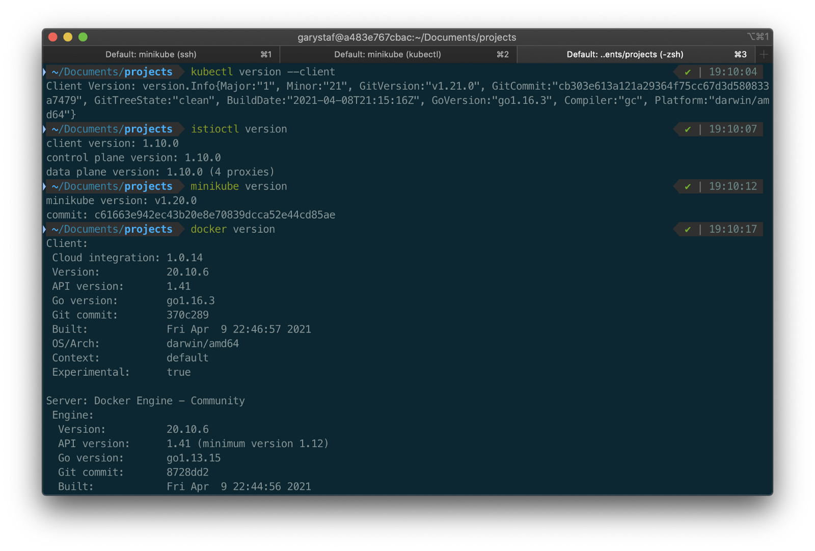
This post will assume a basic level of knowledge of Kubernetes, minikube, Docker, and Istio. Furthermore, the post assumes you have already installed recent versions of minikube, kubectl, Docker, and Istio. Meaning, that the kubectl, istioctl, docker, and minikube commands are all available from the terminal.
For this post demonstration, I am using an Apple MacBook Pro running macOS as my development machine. I have the latest versions of Docker Desktop, minikube, kubectl, and Istio installed as of May 2021.
Source Code
The source code for this post is open-source and is publicly available on GitHub. Clone the GitHub project using the following command:
clone --branch 2021-istio \
    --single-branch --depth 1 \
    https://github.com/garystafford/storefront-demo.git
Minikube
Part of the Kubernetes project, minikube is local Kubernetes, focusing on making it easy to learn and develop for Kubernetes. Minikube quickly sets up a local Kubernetes cluster on macOS, Linux, and Windows. Given the number of Kubernetes resources we will be deploying to minikube, I would recommend at least 3 CPUs and 4–5 GBs of memory. If you choose to deploy multiple observability tools, you may want to increase both of these resources if you can afford it. I maxed out both CPUs and memory several times while setting up this demonstration, causing temporary lock-ups of minikube.
minikube --cpus 3 --memory 5g --driver=docker start start

The Docker driver allows you to install Kubernetes into an existing Docker install. If you are using Docker, please be aware that you must have at least an equivalent amount of resources allocated to Docker to apportion to minikube.

Before continuing, confirm minikube is up and running and confirm the current context of kubectl is minikube.
minikube status
kubectl config current-context
The statuses should look similar to the following:

Use the eval below command to point your shell to minikube’s docker-daemon. You can confirm this by using the docker image ls and docker container ls command to view running Kubernetes containers on minikube.
eval $(minikube -p minikube docker-env)
docker image ls
docker container ls
The output should look similar to the following:

You can also check the status of minikube from Docker Desktop. Minikube is running as a container, instantiated from a Docker image, gcr.io/k8s-minikube/kicbase. View the container’s Stats, as shown below.

Istio
Assuming you have downloaded and configured Istio, install it onto minikube. I currently have Istio 1.10.0 installed and have theISTIO_HOME environment variable set in my Oh My Zsh .zshrc file. I have also set Istio’s bin/ subdirectory in my PATH environment variable. The bin/ subdirectory contains the istioctl executable.
echo $ISTIO_HOME
> /Applications/Istio/istio-1.10.0
where istioctl
> /Applications/Istio/istio-1.10.0/bin/istioctl
istioctl version

> client version: 1.10.0
  control plane version: 1.10.0
  data plane version: 1.10.0 (4 proxies)
Istio comes with several built-in configuration profiles. The profiles provide customization of the Istio control plane and of the sidecars for the Istio data plane.
istioctl profile list
> Istio configuration profiles:
    default
    demo
    empty
    external
    minimal
    openshift
    preview
    remote
For this demonstration, we will use the default profile, which installs istiod and an istio-ingressgateway. We will not require the use of an istio-egressgateway, since all components will be installed locally on minikube.
istioctl install --set profile=default -y
> ✔ Istio core installed
  ✔ Istiod installed
  ✔ Ingress gateways installed
  ✔ Installation complete

Minikube Tunnel
kubectl get svc istio-ingressgateway -n istio-system
To associate an IP address, run the minikube tunnel command in a separate terminal tab. Since it requires opening privileged ports 80 and 443 to be exposed, this command will prompt you for your sudo password.
Services of the type LoadBalancer can be exposed by using the minikube tunnel command. It must be run in a separate terminal window to keep the LoadBalancer running. We previously created the istio-ingressgateway. Run the following command and note that the status of EXTERNAL-IP is <pending>. There is currently no external IP address associated with our LoadBalancer.
minikube tunnel
Rerun the previous command. There should now be an external IP address associated with the LoadBalancer. In my case, 127.0.0.1.
kubectl get svc istio-ingressgateway -n istio-system
The external IP address shown is the address we will use to access the resources we chose to expose externally on minikube.
Minikube Dashboard
Once again, in a separate terminal tab, open the Minikube Dashboard (aka Kubernetes Dashboard).
minikube dashboard
The dashboard will give you a visual overview of all your installed Kubernetes components.

Namespaces
Kubernetes supports multiple virtual clusters backed by the same physical cluster. These virtual clusters are called namespaces. For this demonstration, we will use four namespaces to organize our deployed resources: dev, mongo, kafka, and storefront-kafka-project. The dev namespace is where we will deploy our Storefront API’s microservices: accounts, orders, and fulfillment. We will deploy MongoDB and Mongo Express to the mongo namespace. Lastly, we will use the kafka and storefront-kafka-project namespaces to deploy Apache Kafka to minikube using Strimzi, a Cloud Native Computing Foundation sandbox project, and CMAK.
kubectl apply -f ./minikube/resources/namespaces.yaml
Automatic Sidecar Injection
In order to take advantage of all of Istio’s features, pods in the mesh must be running an Istio sidecar proxy. When you set the istio-injection=enabled label on a namespace and the injection webhook is enabled, any new pods created in that namespace will automatically have a sidecar added to them. Labeling the dev namespace for automatic sidecar injection ensures that our Storefront API’s microservices — accounts, orders, and fulfillment— will have Istio sidecar proxy automatically injected into their pods.
kubectl label namespace dev istio-injection=enabled
MongoDB
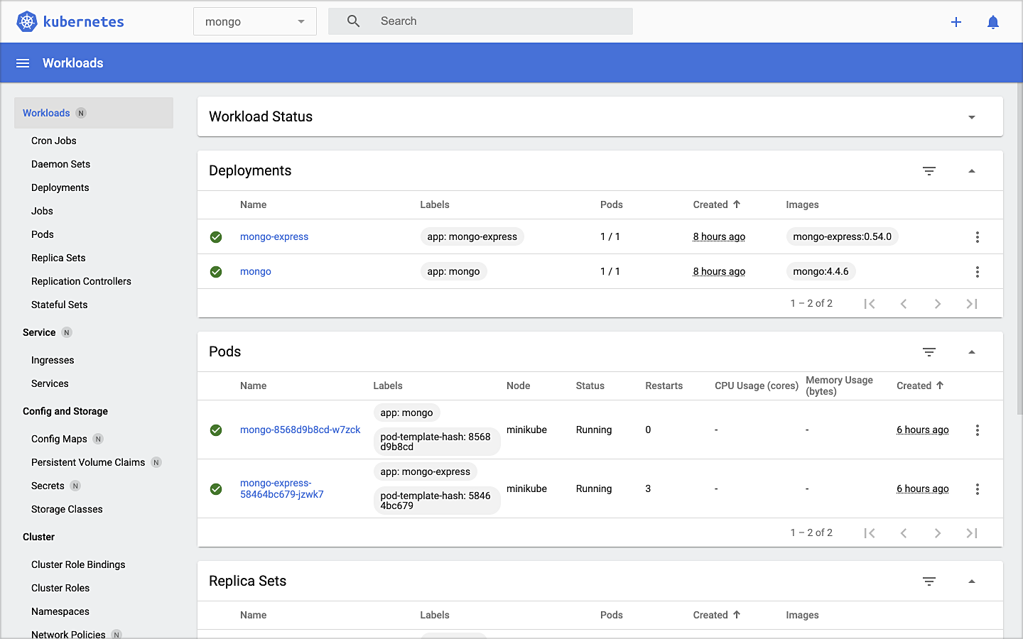
Next, deploy MongoDB and Mongo Express to the mongo namespace on minikube. To ensure a successful connection to MongoDB from Mongo Express, I suggest giving MongoDB a chance to start up fully before deploying Mongo Express.
kubectl apply -f ./minikube/resources/mongodb.yaml -n mongo
sleep 60
kubectl apply -f ./minikube/resources/mongo-express.yaml -n mongo
To confirm the success of the deployments, use the following command:
kubectl get services -n mongo
Or use the Kubernetes Dashboard to confirm deployments.
Mongo Express UI Access
For parts of your application (for example, frontends) you may want to expose a Service onto an external IP address outside of your cluster. Kubernetes ServiceTypes allows you to specify what kind of Service you want; the default is ClusterIP.
Note that while MongoDB uses the ClusterIP, Mongo Express uses NodePort. With NodePort, the Service is exposed on each Node’s IP at a static port (the NodePort). You can contact the NodePort Service, from outside the cluster, by requesting <NodeIP>:<NodePort>.
In a separate terminal tab, open Mongo Express using the following command:
minikube service --url mongo-express -n mongo
You should see output similar to the following:

Click on the link to open Mongo Express. There should already be three MongoDB operational databases shown in the UI. The three Storefront databases and collections will be created automatically, later in the post: accounts, orders, and fulfillment.

Apache Kafka using Strimzi
Next, we will install Apache Kafka and Apache Zookeeper into the kafka and storefront-kafka-project namespaces on minikube, using Strimzi. Since Strimzi has a great, easy-to-use Quick Start guide, I will not detail the complete install complete process in this post. I suggest using their guide to understand the process and what each command does. Then, use the slightly modified Strimzi commands I have included below to install Kafka and Zookeeper.
# assuming 0.23.0 is latest version available
curl -L -O https://github.com/strimzi/strimzi-kafka-operator/releases/download/0.23.0/strimzi-0.23.0.zip
unzip strimzi-0.23.0.zip
cd strimzi-0.23.0
sed -i '' 's/namespace: .*/namespace: kafka/' install/cluster-operator/*RoleBinding*.yaml
# manually change STRIMZI_NAMESPACE value to storefront-kafka-project
nano install/cluster-operator/060-Deployment-strimzi-cluster-operator.yaml
kubectl create -f install/cluster-operator/ -n kafka
kubectl create -f install/cluster-operator/020-RoleBinding-strimzi-cluster-operator.yaml -n storefront-kafka-project
kubectl create -f install/cluster-operator/032-RoleBinding-strimzi-cluster-operator-topic-operator-delegation.yaml -n storefront-kafka-project
kubectl create -f install/cluster-operator/031-RoleBinding-strimzi-cluster-operator-entity-operator-delegation.yaml -n storefront-kafka-project
kubectl apply -f ../storefront-demo/minikube/resources/strimzi-kafka-cluster.yaml -n storefront-kafka-project
kubectl wait kafka/kafka-cluster --for=condition=Ready --timeout=300s -n storefront-kafka-project
kubectl apply -f ../storefront-demo/minikube/resources/strimzi-kafka-topics.yaml -n storefront-kafka-project
Zoo Entrance
We want to install Yahoo’s CMAK (Cluster Manager for Apache Kafka) to give us a management interface for Kafka. However, CMAK required access to Zookeeper. You can not access Strimzi’s Zookeeper directly from CMAK; this is intentional to avoid performance and security issues. See this GitHub issue for a better explanation of why. We will use the appropriately named Zoo Entrance as a proxy for CMAK to Zookeeper to overcome this challenge.
To install Zoo Entrance, review the GitHub project’s install guide, then use the following commands:
git clone https://github.com/scholzj/zoo-entrance.git
cd zoo-entrance
# optional: change my-cluster to kafka-cluster
sed -i '' 's/my-cluster/kafka-cluster/' deploy.yaml
kubectl apply -f deploy.yaml -n storefront-kafka-project
Cluster Manager for Apache Kafka
Next, install Yahoo’s CMAK (Cluster Manager for Apache Kafka) to give us a management interface for Kafka. Run the following command to deploy CMAK into the storefront-kafka-project namespace.
kubectl apply -f ./minikube/resources/cmak.yaml -n storefront-kafka-project

Similar to Mongo Express, we can access CMAK’s UI using its NodePort. In a separate terminal tab, run the following command:
minikube service --url cmak -n storefront-kafka-project
You should see output similar to Mongo Express. Click on the link provided to access CMAK. Choose ‘Add Cluster’ in CMAK to add our existing Kafka cluster to CMAK’s management interface. Use Zoo Enterence’s service address for the Cluster Zookeeper Hosts value.
zoo-entrance.storefront-kafka-project.svc:2181

Once complete, you should see the three Kafka topics we created previously with Strimzi: accounts.customer.change, fulfillment.order.change, and orders.order.change. Each topic will have three partitions, one replica, and one broker. You should also see the _consumer_offsets topic that Kafka uses to store information about committed offsets for each topic:partition per group of consumers (groupID).

Storefront API Microservices
We are finally ready to install our Storefront API’s microservices into the dev namespace. Each service is preconfigured to access Kafka and MongoDB in their respective namespaces.
kubectl apply -f ./minikube/resources/accounts.yaml -n dev
kubectl apply -f ./minikube/resources/orders.yaml -n dev
kubectl apply -f ./minikube/resources/fulfillment.yaml -n dev
Spring Boot services usually take about two minutes to fully start. The time required to download the Docker Images from docker.com and the start-up time means it could take 3–4 minutes for each of the three services to be ready to accept API traffic.

Istio Components
We want to be able to access our Storefront API’s microservices through our Kubernetes LoadBalancer, while also leveraging all the capabilities of Istio as a service mesh. To do so, we need to deploy an Istio Gateway and a VirtualService. We will also need to deploy DestinationRule resources. A Gateway describes a load balancer operating at the edge of the mesh receiving incoming or outgoing HTTP/TCP connections. A VirtualService defines a set of traffic routing rules to apply when a host is addressed. Lastly, a DestinationRule defines policies that apply to traffic intended for a Service after routing has occurred.
kubectl apply -f ./minikube/resources/destination_rules.yaml -n dev
kubectl apply -f ./minikube/resources/istio-gateway.yaml -n dev
Testing the System and Creating Sample Data
I have provided a Python 3 script that runs a series of seven HTTP GET requests, in a specific order, against the Storefront API. These calls will validate the deployments, confirm the API’s services can access Kafka and MongoDB, generate some initial data, and automatically create the MongoDB database collections from the initial Insert statements.
python3 -m pip install -r ./utility_scripts/requirements.txt -U
python3 ./utility_scripts/refresh.py
The script’s output should be as follows:

If we now look at Mongo Express, we should note three new databases: accounts, orders, and fulfillment.

Observability Tools
Istio makes it easy to integrate with a number of common tools, including cert-manager, Prometheus, Grafana, Kiali, Zipkin, and Jaeger. In order to better observe our Storefront API, we will install three well-known observability tools: Kiali, Prometheus, and Grafana. Luckily, these tools are all included with Istio. You can install any or all of these to minikube. I suggest installing the tools one at a time as not to overwhelm minikube’s CPU and memory resources.
kubectl apply -f ./minikube/resources/prometheus.yaml

kubectl apply -f $ISTIO_HOME/samples/addons/grafana.yaml

kubectl apply -f $ISTIO_HOME/samples/addons/kiali.yaml
Once deployment is complete, to access any of the UI’s for these tools, use the istioctl dashboard command from a new terminal window:
istioctl dashboard kiali

istioctl dashboard prometheus

istioctl dashboard grafana
Kiali
Below we see a view of Kiali with API traffic flowing to Kafka and MongoDB.

Prometheus
Each of the three Storefront API microservices has a dependency on Micrometer; specifically, a dependency on micrometer-registry-prometheus. As an instrumentation facade, Micrometer allows you to instrument your code with dimensional metrics with a vendor-neutral interface and decide on the monitoring system as a last step. Instrumenting your core library code with Micrometer allows the libraries to be included in applications that ship metrics to different backends. Given the Micrometer Prometheus dependency, each microservice exposes a /prometheus endpoint (e.g., http://127.0.0.1/accounts/actuator/prometheus) as shown below in Postman.

The /prometheus endpoint exposes dozens of useful metrics and is configured to be scraped by Prometheus. These metrics can be displayed in Prometheus and indirectly in Grafana dashboards via Prometheus. I have customized Istio’s version of Prometheus and included it in the project (prometheus.yaml), which now scrapes the Storefront API’s metrics.
scrape_configs:
    - job_name: 'spring_micrometer'
      metrics_path: '/actuator/prometheus'
      scrape_interval: 5s
      static_configs:
        - targets: ['accounts.dev:8080','orders.dev:8080','fulfillment.dev:8080']
Here we see an example graph of a Spring Kafka Listener metric, spring_kafka_listener_seconds_sum, in Prometheus. There are dozens of metrics exposed to Prometheus from our system that we can observe and alert on.

Grafana
Lastly, here is an example Spring Boot Dashboard in Grafana. More dashboards are available on Grafana’s community dashboard page. The Grafana dashboard uses Prometheus as the source of its metrics data.

Storefront API Endpoints
The three storefront services are fully functional Spring Boot, Spring Data REST, Spring HATEOAS-enabled applications. Each service exposes a rich set of CRUD endpoints for interacting with the service’s data entities. To better understand the Storefront API, each Spring Boot microservice uses SpringFox, which produces automated JSON API documentation for APIs built with Spring. The service builds also include the springfox-swagger-ui web jar, which ships with Swagger UI. Swagger takes the manual work out of API documentation, with a range of solutions for generating, visualizing, and maintaining API docs.
From a web browser, you can use the /swagger-ui/ subdirectory/subpath with any of the three microservices to access the fully-featured Swagger UI (e.g., http://127.0.0.1/accounts/swagger-ui/).

Each service’s data model (POJOs) is also exposed through the Swagger UI.

Spring Boot Actuator
Additionally, each service includes Spring Boot Actuator. The Actuator exposes additional operational endpoints, allowing us to observe the running services. With Actuator, you get many features, including access to available operational-oriented endpoints, using the /actuator/ subdirectory/subpath (e.g., http://127.0.0.1/accounts/actuator/). For this demonstration, I have not restricted access to any available Actuator endpoints.


Conclusion
In this two-part post, we learned how to build an API using Spring Boot. We ensured the API’s distributed data integrity using a pub/sub model with Spring for Apache Kafka Project. When a relevant piece of data was changed by one microservice, that state change triggered a state change event that was shared with other microservices using Kafka topics.
We also learned how to deploy and run the API in a local development environment running on Kubernetes with Istio, using minikube. We have added production-tested observability tools to provide operational visibility, including CMAK, Mongo Express, Kiali, Prometheus, and Grafana.
This blog represents my own viewpoints and not of my employer, Amazon Web Services (AWS). All product names, logos, and brands are the property of their respective owners.
IoT Telemetry Collection using Google Protocol Buffers, Google Cloud Functions, Cloud Pub/Sub, and MongoDB Atlas
Posted by Gary A. Stafford in Big Data, Cloud, GCP, Python, Serverless, Software Development on May 21, 2019

Collect IoT sensor telemetry using Google Protocol Buffers’ serialized binary format over HTTPS, serverless Google Cloud Functions, Google Cloud Pub/Sub, and MongoDB Atlas on GCP, as an alternative to integrated Cloud IoT platforms and standard IoT protocols. Aggregate, analyze, and build machine learning models with the data using tools such as MongoDB Compass, Jupyter Notebooks, and Google’s AI Platform Notebooks.
Introduction
Most of the dominant Cloud providers offer IoT (Internet of Things) and IIotT (Industrial IoT) integrated services. Amazon has AWS IoT, Microsoft Azure has multiple offering including IoT Central, IBM’s offering including IBM Watson IoT Platform, Alibaba Cloud has multiple IoT/IIoT solutions for different vertical markets, and Google offers Google Cloud IoT platform. All of these solutions are marketed as industrial-grade, highly-performant, scalable technology stacks. They are capable of scaling to tens-of-thousands of IoT devices or more and massive amounts of streaming telemetry.
In reality, not everyone needs a fully integrated IoT solution. Academic institutions, research labs, tech start-ups, and many commercial enterprises want to leverage the Cloud for IoT applications, but may not be ready for a fully-integrated IoT platform or are resistant to Cloud vendor platform lock-in.
Similarly, depending on the performance requirements and the type of application, organizations may not need or want to start out using IoT/IIOT industry standard data and transport protocols, such as MQTT (Message Queue Telemetry Transport) or CoAP (Constrained Application Protocol), over UDP (User Datagram Protocol). They may prefer to transmit telemetry over HTTP using TCP, or securely, using HTTPS (HTTP over TLS).
Demonstration
In this demonstration, we will collect environmental sensor data from a number of IoT device sensors and stream that telemetry over the Internet to Google Cloud. Each IoT device is installed in a different physical location. The devices contain a variety of common sensors, including humidity and temperature, motion, and light intensity.

Prototype IoT Devices used in this Demonstration
We will transmit the sensor telemetry data as JSON over HTTP to serverless Google Cloud Function HTTPS endpoints. We will then switch to using Google’s Protocol Buffers to transmit binary data over HTTP. We should observe a reduction in the message size contained in the request payload as we move from JSON to Protobuf, which should reduce system latency and cost.
Data received by Cloud Functions over HTTP will be published asynchronously to Google Cloud Pub/Sub. A second Cloud Function will respond to all published events and push the messages to MongoDB Atlas on GCP. Once in Atlas, we will aggregate, transform, analyze, and build machine learning models with the data, using tools such as MongoDB Compass, Jupyter Notebooks, and Google’s AI Platform Notebooks.
For this demonstration, the architecture for JSON over HTTP will look as follows. All sensors will transmit data to a single Cloud Function HTTPS endpoint.
![]()
For Protobuf over HTTP, the architecture will look as follows in the demonstration. Each type of sensor will transmit data to a different Cloud Function HTTPS endpoint.
![]()
Although the Cloud Functions will automatically scale horizontally to accommodate additional load created by the volume of telemetry being received, there are also other options to scale the system. For example, we could create individual pipelines of functions and topic/subscriptions for each sensor type. We could also split the telemetry data across multiple MongoDB Atlas Collections, based on sensor type, instead of a single collection. In all cases, we will still benefit from the Cloud Function’s horizontal scaling capabilities.
![]()
Source Code
All source code is all available on GitHub. Use the following command to clone the project.
git clone \
  --branch master --single-branch --depth 1 --no-tags \
  https://github.com/garystafford/iot-protobuf-demo.git
You will need to adjust the project’s environment variables to fit your own development and Cloud environments. All source code for this post is written in Python. It is intended for Python 3 interpreters but has been tested using Python 2 interpreters. The project’s Jupyter Notebooks can be viewed from within the project on GitHub or using the free, online Jupyter nbviewer.

Technologies
Protocol Buffers
 According to Google, Protocol Buffers (aka Protobuf) are a language- and platform-neutral, efficient, extensible, automated mechanism for serializing structured data for use in communications protocols, data storage, and more. Protocol Buffers are 3 to 10 times smaller and 20 to 100 times faster than XML.
Each protocol buffer message is a small logical record of information, containing a series of strongly-typed name-value pairs. Once you have defined your messages, you run the protocol buffer compiler for your application’s language on your .proto file to generate data access classes.
Google Cloud Functions

According to Google, Cloud Functions is Google’s event-driven, serverless compute platform. Key features of Cloud Functions include automatic scaling, high-availability, fault-tolerance,
no servers to provision, manage, patch or update, only
pay while your code runs, and they easily connect and extend other cloud services. Cloud Functions natively support multiple event-types, including HTTP, Cloud Pub/Sub, Cloud Storage, and Firebase. Current language support includes Python, Go, and Node.
Google Cloud Pub/Sub
 According to Google, Cloud Pub/Sub is an enterprise message-oriented middleware for the Cloud. It is a scalable, durable event ingestion and delivery system. By providing many-to-many, asynchronous messaging that decouples senders and receivers, it allows for secure and highly available communication among independent applications. Cloud Pub/Sub delivers low-latency, durable messaging that integrates with systems hosted on the Google Cloud Platform and externally.
MongoDB Atlas
 MongoDB Atlas is a fully-managed MongoDB-as-a-Service, available on AWS, Azure, and GCP. Atlas, a mature SaaS product, offers high-availability, uptime service-level agreements, elastic scalability, cross-region replication, enterprise-grade security, LDAP integration, BI Connector, and much more.
MongoDB Atlas currently offers four pricing plans, Free, Basic, Pro, and Enterprise. Plans range from the smallest, free M0-sized MongoDB cluster, with shared RAM and 512 MB storage, up to the massive M400 MongoDB cluster, with 488 GB of RAM and 3 TB of storage.
Cost Effectiveness of Cloud Functions
At true IIoT scale, Google Cloud Functions may not be the most efficient or cost-effective method of ingesting telemetry data. Based on Google’s pricing model, you get two million free function invocations per month, with each additional million invocations costing USD $0.40. The total cost also includes memory usage, total compute time, and outbound data transfer. If your system is comprised of tens or hundreds of IoT devices, Cloud Functions may prove cost-effective.
However, with thousands of devices or more, each transmitting data multiple times per minutes, you could quickly outgrow the cost-effectiveness of Google Functions. In that case, you might look to Google’s Google Cloud IoT platform. Alternately, you can build your own platform with Google products such as Knative, letting you choose to run your containers either fully managed with the newly-released Cloud Run, or in your Google Kubernetes Engine cluster with Cloud Run on GKE.
Sensor Scripts
For each sensor type, I have developed separate Python scripts, which run on each IoT device. There are two versions of each script, one for JSON over HTTP and one for Protobuf over HTTP.
JSON over HTTPS
Below we see the script, dht_sensor_http_json.py, used to transmit humidity and temperature data via JSON over HTTP to a Google Cloud Function running on GCP. The JSON request payload contains a timestamp, IoT device ID, device type, and the temperature and humidity sensor readings. The URL for the Google Cloud Function is stored as an environment variable, local to the IoT devices, and set when the script is deployed.
import json
import logging
import os
import socket
import sys
import time

import Adafruit_DHT
import requests

URL = os.environ.get('GCF_URL')
JWT = os.environ.get('JWT')
SENSOR = Adafruit_DHT.DHT22
TYPE = 'DHT22'
PIN = 18
FREQUENCY = 15


def main():
    if not URL or not JWT:
        sys.exit("Are the Environment Variables set?")
    get_sensor_data(socket.gethostname())


def get_sensor_data(device_id):
    while True:
        humidity, temperature = Adafruit_DHT.read_retry(SENSOR, PIN)
        payload = {'device': device_id,
                   'type': TYPE,
                   'timestamp': time.time(),
                   'data': {'temperature': temperature,
                            'humidity': humidity}}
        post_data(payload)
        time.sleep(FREQUENCY)


def post_data(payload):
    payload = json.dumps(payload)

    headers = {
        'Content-Type': 'application/json; charset=utf-8',
        'Authorization': JWT
    }

    try:
        requests.post(URL, json=payload, headers=headers)
    except requests.exceptions.ConnectionError:
        logging.error('Error posting data to Cloud Function!')
    except requests.exceptions.MissingSchema:
        logging.error('Error posting data to Cloud Function! Are Environment Variables set?')


if __name__ == '__main__':
    sys.exit(main())
Telemetry Frequency
Although the sensors are capable of producing data many times per minute, for this demonstration, sensor telemetry is intentionally limited to only being transmitted every 15 seconds. To reduce system complexity, potential latency, back-pressure, and cost, in my opinion, you should only produce telemetry data at the frequency your requirements dictate.
JSON Web Tokens
For security, in addition to the HTTPS endpoints exposed by the Google Cloud Functions, I have incorporated the use of a JSON Web Token (JWT). JSON Web Tokens are an open, industry standard RFC 7519 method for representing claims securely between two parties. In this case, the JWT is used to verify the identity of the sensor scripts sending telemetry to the Cloud Functions. The JWT contains an id, password, and expiration, all encrypted with a secret key, which is known to each Cloud Function, in order to verify the IoT device’s identity. Without the correct JWT being passed in the Authorization header, the request to the Cloud Function will fail with an HTTP status code of 401 Unauthorized. Below is an example of the JWT’s payload data.
{
  "sub": "IoT Protobuf Serverless Demo",
  "id": "iot-demo-key",
  "password": "t7J2gaQHCFcxMD6584XEpXyzWhZwRrNJ",
  "iat": 1557407124,
  "exp": 1564664724
}
For this demonstration, I created a temporary JWT using jwt.io. The HTTP Functions are using PyJWT, a Python library which allows you to encode and decode the JWT. The PyJWT library allows the Function to decode and validate the JWT (Bearer Token) from the incoming request’s Authorization header. The JWT token is stored as an environment variable. Deployment instructions are included in the GitHub project.

JSON Payload
Below is a typical JSON request payload (pretty-printed), containing DHT sensor data. This particular message is 148 bytes in size. The message format is intentionally reader-friendly. We could certainly shorten the message’s key fields, to reduce the payload size by an additional 15-20 bytes.
{
  "device": "rp829c7e0e",
  "type": "DHT22",
  "timestamp": 1557585090.476025,
  "data": {
    "temperature": 17.100000381469727,
    "humidity": 68.0999984741211
  }
}
Protocol Buffers
For the demonstration, I have built a Protocol Buffers file, sensors.proto, to support the data output by three sensor types: digital humidity and temperature (DHT), passive infrared sensor (PIR), and digital light intensity (DLI). I am using the newer proto3 version of the protocol buffers language. I have created a common Protobuf sensor message schema, with the variable sensor telemetry stored in the nested data object, within each message type.
It is important to use the correct Protobuf Scalar Value Type to maintain numeric precision in the language you compile for. For simplicity, I am using a double to represent the timestamp, as well as the numeric humidity and temperature readings. Alternately, you could choose Google’s Protobuf WellKnownTypes, Timestamp to store timestamp.
syntax = "proto3";

package sensors;

// DHT22
message SensorDHT {
    string device = 1;
    string type = 2;
    double timestamp = 3;
    DataDHT data = 4;
}

message DataDHT {
    double temperature = 1;
    double humidity = 2;
}

// Onyehn_PIR
message SensorPIR {
    string device = 1;
    string type = 2;
    double timestamp = 3;
    DataPIR data = 4;
}

message DataPIR {
    bool motion = 1;
}

// Anmbest_MD46N
message SensorDLI {
    string device = 1;
    string type = 2;
    double timestamp = 3;
    DataDLI data = 4;
}

message DataDLI {
    bool light = 1;
}
Since the sensor data will be captured with scripts written in Python 3, the Protocol Buffers file is compiled for Python, resulting in the file, sensors_pb2.py.
protoc --python_out=. sensors.proto
Protocol Buffers over HTTPS
Below we see the alternate DHT sensor script, dht_sensor_http_pb.py, which transmits a Protocol Buffers-based binary request payload over HTTPS to a Google Cloud Function running on GCP. Note the request’s Content-Type header has been changed from application/json to application/x-protobuf. In this case, instead of JSON, the same data fields are stored in an instance of the Protobuf’s SensorDHT message type (sensors_pb2.SensorDHT()). Note the import sensors_pb2 statement. This statement imports the compiled Protocol Buffers file, which is stored locally to the script on the IoT device.
import logging
import os
import socket
import sys
import time

import Adafruit_DHT
import requests
import sensors_pb2

URL = os.environ.get('GCF_DHT_URL')
JWT = os.environ.get('JWT')
SENSOR = Adafruit_DHT.DHT22
TYPE = 'DHT22'
PIN = 18
FREQUENCY = 15


def main():
    if not URL or not JWT:
        sys.exit("Are the Environment Variables set?")
    get_sensor_data(socket.gethostname())


def get_sensor_data(device_id):
    while True:
        try:
            humidity, temperature = Adafruit_DHT.read_retry(SENSOR, PIN)

            sensor_dht = sensors_pb2.SensorDHT()
            sensor_dht.device = device_id
            sensor_dht.type = TYPE
            sensor_dht.timestamp = time.time()
            sensor_dht.data.temperature = temperature
            sensor_dht.data.humidity = humidity

            payload = sensor_dht.SerializeToString()

            post_data(payload)
            time.sleep(FREQUENCY)
        except TypeError:
            logging.error('Error getting sensor data!')


def post_data(payload):
    headers = {
        'Content-Type': 'application/x-protobuf',
        'Authorization': JWT
    }

    try:
        requests.post(URL, data=payload, headers=headers)
    except requests.exceptions.ConnectionError:
        logging.error('Error posting data to Cloud Function!')
    except requests.exceptions.MissingSchema:
        logging.error('Error posting data to Cloud Function! Are Environment Variables set?')


if __name__ == '__main__':
    sys.exit(main())
Protobuf Binary Payload
To understand the binary Protocol Buffers-based payload, we can write a sample SensorDHT message to a file on disk as a byte array.
message = sensorDHT.SerializeToString()

binary_file_output = open("./data_binary.txt", "wb")
file_byte_array = bytearray(message)
binary_file_output.write(file_byte_array)
Then, using the hexdump command, we can view a representation of the binary data file.
> hexdump -C data_binary.txt
00000000  0a 08 38 32 39 63 37 65  30 65 12 05 44 48 54 32  |..829c7e0e..DHT2|
00000010  32 1d 05 a0 b9 4e 22 0a  0d ec 51 b2 41 15 cd cc  |2....N"...Q.A...|
00000020  38 42                                             |8B|
00000022
The binary data file size is 48 bytes on disk, as compared to the equivalent JSON file size of 148 bytes on disk (32% the size). As a test, we could then send that binary data file as the payload of a POST to the Cloud Function, as shown below using Postman. Postman will serialize the binary data file’s contents to a binary string before transmitting.

Similarly, we can serialize the same binary Protocol Buffers-based SensorDHT message to a binary string using the SerializeToString method.
message = sensorDHT.SerializeToString()
print(message)
The resulting binary string resembles the following.
b'\n\nrp829c7e0e\x12\x05DHT22\x19c\xee\xbcg\xf5\x8e\xccA"\x12\t\x00\x00\x00\xa0\x99\x191@\x11\x00\x00\x00`f\x06Q@'
The binary string length of the serialized message, and therefore the request payload sent by Postman and received by the Cloud Function for this particular message, is 111 bytes, as compared to the JSON payload size of 148 bytes (75% the size).
Validate Protobuf Payload
To validate the data contained in the Protobuf payload is identical to the JSON payload, we can parse the payload from the serialized binary string using the Protobuf ParseFromString method. We then convert it to JSON using the Protobuf MessageToJson method.
message = sensorDHT.SerializeToString()
message_parsed = sensors_pb2.SensorDHT()
message_parsed.ParseFromString(message)
print(MessageToJson(message_parsed))
The resulting JSON object is identical to the JSON payload sent using JSON over HTTPS, earlier in the demonstration.
{
  "device": "rp829c7e0e",
  "type": "DHT22",
  "timestamp": 1557585090.476025,
  "data": {
    "temperature": 17.100000381469727,
    "humidity": 68.0999984741211
  }
}
Google Cloud Functions
There are a series of Google Cloud Functions, specifically four HTTP Functions, which accept the sensor data over HTTP from the IoT devices. Each function exposes an HTTPS endpoint. According to Google, you use HTTP functions when you want to invoke your function via an HTTP(S) request. To allow for HTTP semantics, HTTP function signatures accept HTTP-specific arguments.
Below, I have deployed a single function that accepts JSON sensor telemetry from all sensor types, and three functions for Protobuf, one for each sensor type: DHT, PIR, and DLI.

JSON Message Processing
Below, we see the Cloud Function, main.py, which processes the incoming JSON over HTTPS payload from all sensor types. Once the request’s JWT is validated, the JSON message payload is serialized to a byte string and sent to a common Google Cloud Pub/Sub Topic. Note the JWT secret key, id, and password, and the Google Cloud Pub/Sub Topic are all stored as environment variables, local to the Cloud Functions. In my tests, the JSON-based HTTP Functions took an average of 9–18 ms to execute successfully.
import logging
import os

import jwt
from flask import make_response, jsonify
from flask_api import status
from google.cloud import pubsub_v1

TOPIC = os.environ.get('TOPIC')
SECRET_KEY = os.getenv('SECRET_KEY')
ID = os.getenv('ID')
PASSWORD = os.getenv('PASSWORD')


def incoming_message(request):
    if not validate_token(request):
        return make_response(jsonify({'success': False}),
                             status.HTTP_401_UNAUTHORIZED,
                             {'ContentType': 'application/json'})

    request_json = request.get_json()
    if not request_json:
        return make_response(jsonify({'success': False}),
                             status.HTTP_400_BAD_REQUEST,
                             {'ContentType': 'application/json'})

    send_message(request_json)

    return make_response(jsonify({'success': True}),
                         status.HTTP_201_CREATED,
                         {'ContentType': 'application/json'})


def validate_token(request):
    auth_header = request.headers.get('Authorization')
    if not auth_header:
        return False
    auth_token = auth_header.split(" ")[1]

    if not auth_token:
        return False
    try:
        payload = jwt.decode(auth_token, SECRET_KEY)
        if payload['id'] == ID and payload['password'] == PASSWORD:
            return True
    except jwt.ExpiredSignatureError:
        return False
    except jwt.InvalidTokenError:
        return False


def send_message(message):
    publisher = pubsub_v1.PublisherClient()
    publisher.publish(topic=TOPIC,
                      data=bytes(str(message), 'utf-8'))
The Cloud Functions are deployed to GCP using the gcloud functions deploy CLI command (I use Jenkins to automate the deployments). I have wrapped the deploy commands into bash scripts. The script also copies over a common environment variables YAML file, consumed by the Cloud Function. Each Function has a deployment script, included in the project.
# get latest env vars file
cp -f ./../env_vars_file/env.yaml .

# deploy function
gcloud functions deploy http_json_to_pubsub \
  --runtime python37 \
  --trigger-http \
  --region us-central1 \
  --memory 256 \
  --entry-point incoming_message \
  --env-vars-file env.yaml
Using a .gcloudignore file, the gcloud functions deploy CLI command deploys three files: the cloud function (main.py), required Python packages file (requirements.txt), the environment variables file (env.yaml). Google automatically installs dependencies using the requirements.txt file.
Protobuf Message Processing
Below, we see the Cloud Function, main.py, which processes the incoming Protobuf over HTTPS payload from DHT sensor types. Once the sensor data Protobuf message payload is received by the HTTP Function, it is deserialized to JSON and then serialized to a byte string. The byte string is then sent to a Google Cloud Pub/Sub Topic. In my tests, the Protobuf-based HTTP Functions took an average of 7–14 ms to execute successfully.
As before, note the import sensors_pb2 statement. This statement imports the compiled Protocol Buffers file, which is stored locally to the script on the IoT device. It is used to parse a serialized message into its original Protobuf’s SensorDHT message type.
import logging
import os

import jwt
import sensors_pb2
from flask import make_response, jsonify
from flask_api import status
from google.cloud import pubsub_v1
from google.protobuf.json_format import MessageToJson

TOPIC = os.environ.get('TOPIC')
SECRET_KEY = os.getenv('SECRET_KEY')
ID = os.getenv('ID')
PASSWORD = os.getenv('PASSWORD')


def incoming_message(request):
    if not validate_token(request):
        return make_response(jsonify({'success': False}),
                             status.HTTP_401_UNAUTHORIZED,
                             {'ContentType': 'application/json'})

    data = request.get_data()
    if not data:
        return make_response(jsonify({'success': False}),
                             status.HTTP_400_BAD_REQUEST,
                             {'ContentType': 'application/json'})

    sensor_pb = sensors_pb2.SensorDHT()
    sensor_pb.ParseFromString(data)
    sensor_json = MessageToJson(sensor_pb)
    send_message(sensor_json)

    return make_response(jsonify({'success': True}),
                         status.HTTP_201_CREATED,
                         {'ContentType': 'application/json'})


def validate_token(request):
    auth_header = request.headers.get('Authorization')
    if not auth_header:
        return False
    auth_token = auth_header.split(" ")[1]

    if not auth_token:
        return False
    try:
        payload = jwt.decode(auth_token, SECRET_KEY)
        if payload['id'] == ID and payload['password'] == PASSWORD:
            return True
    except jwt.ExpiredSignatureError:
        return False
    except jwt.InvalidTokenError:
        return False


def send_message(message):
    publisher = pubsub_v1.PublisherClient()
    publisher.publish(topic=TOPIC, data=bytes(message, 'utf-8'))
Cloud Pub/Sub Functions
In addition to HTTP Functions, the demonstration uses a function triggered by Google Cloud Pub/Sub Triggers. According to Google, Cloud Functions can be triggered by messages published to Cloud Pub/Sub Topics in the same GCP project as the function. The function automatically subscribes to the Topic. Below, we see that the function has automatically subscribed to iot-data-demo Cloud Pub/Sub Topic.

Sending Telemetry to MongoDB Atlas
The common Cloud Function, triggered by messages published to Cloud Pub/Sub, then sends the messages to MongoDB Atlas. There is a minimal amount of cleanup required to re-format the Cloud Pub/Sub messages to BSON (binary JSON). Interestingly, according to bsonspec.org, BSON can be compared to binary interchange formats, like Protocol Buffers. BSON is more schema-less than Protocol Buffers, which can give it an advantage in flexibility but also a slight disadvantage in space efficiency (BSON has overhead for field names within the serialized data).
The function uses the PyMongo to connect to MongoDB Atlas. According to their website, PyMongo is a Python distribution containing tools for working with MongoDB and is the recommended way to work with MongoDB from Python.
import base64
import json
import logging
import os
import pymongo

MONGODB_CONN = os.environ.get('MONGODB_CONN')
MONGODB_DB = os.environ.get('MONGODB_DB')
MONGODB_COL = os.environ.get('MONGODB_COL')


def read_message(event, context):
    message = base64.b64decode(event['data']).decode('utf-8')
    message = message.replace("'", '"')
    message = message.replace('True', 'true')
    message = json.loads(message)

    client = pymongo.MongoClient(MONGODB_CONN)
    db = client[MONGODB_DB]
    col = db[MONGODB_COL]
    col.insert_one(message)
The function responds to the published events and sends the messages to the MongoDB Atlas cluster, running in the same Region, us-central1, as the Cloud Functions and Pub/Sub Topic. Below, we see the current options available when provisioning an Atlas cluster.

MongoDB Atlas provides a rich, web-based UI for managing and monitoring MongoDB clusters, databases, collections, security, and performance.

Although Cloud Pub/Sub to Atlas function execution times are longer in duration than the HTTP functions, the latency is greatly reduced by locating the Cloud Pub/Sub Topic, Cloud Functions, and MongoDB Atlas cluster into the same GCP Region. Cross-region execution times were as high as 500-600 ms, while same-region execution times averaged 200-225 ms. Selecting a more performant Atlas cluster would likely result in even lower function execution times.

Aggregating Data with MongoDB Compass
MongoDB Compass is a free, convenient, desktop application for interacting with your MongoDB databases. You can view the collected sensor data, review message (document) schema, manage indexes, and build complex MongoDB aggregations.


When performing analytics or machine learning, I primarily use MongoDB Compass to preview the captured telemetry data and build aggregation pipelines. Aggregation operations process data records and returns computed results. This feature saves a ton of time, filtering and preparing data for further analysis, visualization, and machine learning with Jupyter Notebooks.

Aggregation pipelines can be directly exported to Java, Node, C#, and Python 3. The exported aggregation pipeline code can be placed directly into your Python applications and Jupyter Notebooks.

Below, the exported aggregation pipelines code from MongoDB Compass is used to load a resultset directly into a Pandas DataFrame. This particular aggregation returns time-series DHT sensor data from a specific IoT device over a 72-hour period.
DEVICE_1 = 'rp59adf374'
pipeline = [
    {
        '$match': {
            'type': 'DHT22',
            'device': DEVICE_1,
            'timestamp': {
                '$gt': 1557619200,
                '$lt': 1557792000
            }
        }
    }, {
        '$project': {
            '_id': 0,
            'timestamp': 1,
            'temperature': '$data.temperature',
            'humidity': '$data.humidity'
        }
    }, {
        '$sort': {
            'timestamp': 1
        }
    }
]
aggResult = iot_data.aggregate(pipeline)
df1 = pd.DataFrame(list(aggResult))
MongoDB Atlas Performance
In this demonstration, from Python3-based Jupyter Notebooks, I was able to consistently query a MongoDB Atlas collection of almost 70k documents for resultsets containing 3 days (72 hours) worth of digital temperature and humidity data, roughly 10.2k documents, in an average of 825 ms. That is round trip from my local development laptop to MongoDB Atlas running on GCP, in a different geographic region.
Query times on GCP are much faster, such as when running a Notebook in JupyterLab on Google’s AI Platform, or a PySpark job with Cloud Dataproc, against Atlas. Running the same Jupyter Notebook directly on Google’s AI Platform, the same MongoDB Atlas query took an average of 450 ms versus 825 ms (1.83x faster). This was across two different GCP Regions; same Region times should be even faster.

GCP Observability
There are several choices for observing the system’s Google Cloud Functions, Google Cloud Pub/Sub, and MongoDB Atlas. As shown above, the GCP Cloud Functions interface lets you see the individual function executions, execution times, memory usage, and active instances, over varying time intervals.
For a more detailed view of Google Cloud Functions and Google Cloud Pub/Sub, I built two custom dashboards using Stackdriver. According to Google, Stackdriver aggregates metrics, logs, and events from infrastructure, giving developers and operators a rich set of observable signals. I built a custom Stackdriver Cloud Functions dashboard (shown below) and a Cloud Pub/Sub Topics and Subscriptions dashboard.
For functions, I chose to display execution times, memory usage, the number of executions, and network egress, all in a single pane of glass, using four graphs. Below, I am using the 95th percentile average for monitoring. The 95th percentile asserts that 95% of the time, the observed values are below this amount and the remaining 5% of the time, the observed values are above that amount.

Data Analysis using Jupyter Notebooks
According to jupyter.org, the Jupyter Notebook is an open-source web application that allows you to create and share documents that contain live code, equations, visualizations, and narrative text. Uses include data cleaning and transformation, numerical simulation, statistical modeling, data visualization, machine learning, and much more. The widespread use of Jupyter Notebooks has grown significantly, as Big Data, AI, and ML have all experienced explosive growth.
PyCharm
JetBrains PyCharm, my favorite Python IDE, has direct integrations with Jupyter Notebooks. In fact, PyCharm’s most recent updates to the Professional Edition greatly enhanced those integrations. PyCharm offers round-trip editing in the IDE and the Jupyter Notebook web browser interface. PyCharm allows you to run and debug individual cells within the notebook. PyCharm automatically starts the Jupyter Server and appropriate kernel for the Notebook you have opened. And, one of my favorite features, PyCharm’s variable viewer tracks the current value of a variable, automatically.

Below, we see the example Analytics Notebook, included in the demonstration’s project, displayed in PyCharm 19.1.2 (Professional Edition). To effectively work with Notebooks in PyCharm really requires a full-size monitor. Working on a laptop with PyCharm’s crowded Notebook UI is workable, but certainly not as effective as on a larger monitor.

Jupyter Notebook Server
Below, we see the same Analytics Notebook, shown above in PyCharm, opened in Jupyter Notebook Server’s web-based client interface, running locally on the development workstation. The web browser-based interface also offers a rich set of features for Notebook development.
From within the Notebook, we are able to query the data from MongoDB Atlas, again using PyMongo, and load the resultsets into Panda DataFrames. As an alternative to hard-coded values and environment variables, with Notebooks, I use the python-dotenv Python package. This package allows me to place my environment variables in a common .env file and reference them from any Notebook. The package has many options for managing environment variables.

We can then analyze the data using a number of common frameworks, including Pandas, Matplotlib, SciPy, PySpark, and NumPy, to name but a few. Below, we see time series data from four different sensors, on the same IoT device. Viewing the data together, we can study the causal effect of one environment variable on another, such as the impact of light on temperature or humidity.

Below, we can use histograms to visualize temperature frequencies for
intervals, over time, for a given device location.

Machine Learning using Jupyter Notebooks
In addition to data analytics, we can use Jupyter Notebooks with tools such as scikit-learn to build machine learning models based on our sensor telemetry. Scikit-learn is a set of machine learning tools in Python, built on NumPy, SciPy, and matplotlib. Below, I have used JupyterLab on Google’s AI Platform and scikit-learn to build several models, based on the sensor data.


Using scikit-learn, we can build models to predict such things as which IoT device generated a specific temperature and humidity reading, or the temperature and humidity, given the time of day, device location, and external environment variables, or discover anomalies in the sensor telemetry.
Scikit-learn makes it easy to construct randomized training and test datasets, to build models, using data from multiple IoT devices, as shown below.

The project includes a Jupyter Notebook that demonstrates how to build several ML models using sensor data. Examples of supervised learning algorithms used to build the classification models in this demonstration include Support Vector Machine (SVM), k-nearest neighbors (k-NN), and Random Forest Classifier.

Having data from multiple sensors, we are able to enrich the ML models by adding additional categorical (discrete) features to our training data. For example, we could look at the effect of light, motion, and time of day on temperature and humidity.

Conclusion
Hopefully, this post has demonstrated how to efficiently collect telemetry data from IoT devices using Google Protocol Buffers over HTTPS, serverless Google Cloud Functions, Cloud Pub/Sub, and MongoDB Atlas, all on the Google Cloud Platform. Once captured, the telemetry data was easily aggregated and analyzed using common tools, such as MongoDB Compass and Jupyter Notebooks. Further, we used the data and tools to build machine learning models for prediction and anomaly detection.
All opinions expressed in this post are my own and not necessarily the views of my current or past employers or their clients.
Image: everythingpossible © 123RF.com
Apache Solr: Because your Database is not a Search Engine
Posted by Gary A. Stafford in Python, Software Development on February 25, 2019
In this post, we will examine what sets Apache Solr aside as a search engine, from conventional databases like MongoDB. We will explore the similarities and differences between Solr and MongoDB by analyzing a series of comparative queries. We will then delve into some of Solr’s more advanced search capabilities.

Why Search?
The ability to search for information is a basic requirement of many applications. Architects and Developers who limit themselves to traditional databases, often attempt to meet search requirements by creating unnecessarily and overly complex SQL query-based solutions. They force end-users to search in unnatural or highly-structured ways or provide results that lack a sense of relevancy. End-users are not Database Administrators, they do not understand the nuances of SQL, they simply want relevant responses to their inquiries.
In a scenario where data consumers are arbitrarily searching for relevant information within a distinct domain, implementing a search-optimized, Lucene-based platform, such as Elasticsearch or Apache Solr, for reads, is often an effective solution.
Separating database reads from writes is not uncommon. I’ve worked on many projects where the requirements suggested an architecture in which one type of data storage technology should be implemented to optimize for writes, while a different type or types of data storage technologies should be implemented to optimize for reads. Architectures in which this is common include the following.
- CQRS (Command Query Responsibility Segregation) and Event Sourcing;
- Reporting, Data Analytics, and Big Data;
- ML (Machine Learning) and AI (Artificial Intelligence);
- Real-Time and Streaming Data (such as IoT);
- Search: Content, Document, Knowledge;
In this post, we will examine the search capabilities of Apache Solr. We will compare and contrast Solr’s search capabilities to those of MongoDB, the leading NoSQL database. We will consider the differences between querying for data and searching for information.
Apache Lucene
According to Apache, the Apache Lucene project develops open-source search software, including the following sub-projects: Lucene Core, Solr, and PyLucene. The Lucene Core sub-project provides Java-based indexing and search technology, as well as spellchecking, hit highlighting, and advanced analysis/tokenization capabilities.
Apache Lucene 7.7.0 and Apache Solr 7.7.0 were just released in February 2019 and used for all the post’s examples.
 Apache Solr
According to Apache, Apache Solr is the popular, blazing fast, open source, enterprise search platform built on Apache Lucene. Solr powers the search and navigation features of many of the world’s largest internet sites.
Apache Solr includes the ability to set up a cluster of Solr servers that combines fault tolerance and high availability. Referred to as SolrCloud, and backed by Apache Zookeeper, these capabilities provide distributed, sharded, and replicated indexing and search capabilities.
According to Wikipedia, Solr was created at CNET Networks in 2004, donated to the Apache Software Foundation in 2006, and graduated from their incubator in 2007. Solr version 1.3 was released in 2008. In 2010, the Lucene and Solr projects merged; Solr became a Lucene subproject. With Apache Solr 7.7.0 just released, Solr has well over ten years of development and enterprise adoption behind it.
MongoDB
The leading NoSQL database, MongoDB, describes itself as a document database with the scalability and flexibility that you want with the querying and indexing that users need. Mongo features include ad hoc queries, indexing, and real-time aggregation, which provide powerful ways to access and analyze your data.
Released less than a year ago, MongoDB 4.0 added multi-document ACID transactions, data type conversions, non-blocking secondary replica reads, SHA-2 authentication, MongoDB Compass aggregation pipeline builder, Kubernetes integration, and the MongoDB Stitch serverless platform. MongoDB 4.0.6 was just released in February 2019 and used for all the post’s examples.
Comparing Search Features
Solr and MongoDB appear to have many search-related features in common.
- Both Solr and MongoDB are document-based data stores;
- Both Solr and MongoDB use a non-relational data model;
- Both feature advanced querying and indexing capabilities;
- Solr implements Lucene-based search capabilities; MongoDB has text-based search capabilities;
- Solr scores the relevance of search results using the Lucene scoring algorithm; MongoDB has the capability of ranking text search results using the $meta operator;
- Solr is able to selectively boost the relative importance of search fields and specific values in a field when calculating scores; MongoDB has the capability of boosting the relative importance of fields used in a text search using text indexes;
- Both Solr and MongoDB are capable of implementing stop words, stemming, and tokenization;
Demonstration
Source Code Examples
All examples shown in this post are available as a series of Python 3 scripts, contained in an open-source project on GitHub, searching-solr-vs-mongodb. The project contains the script, query_mongo.py, which uses the Python driver for MongoDB, pymongo, to execute all the MongoDB queries in this post. The project also contains the script, query_solr.py, which uses the lightweight Python wrapper for Apache Solr, pysolr, to execute all the Solr searches in this post. Both packages, along with ancillary packages, may be installed with pip.
pip3 install pysolr pymongo bson.json_util requests
MongoDB and Solr Instances
To follow along, you will need your own MongoDB and Solr instances. Both are easily stood up locally with Docker, using the official MongoDB and Solr Docker Hub images. Example docker run commands are shown below.
The second command, the Solr command, also creates a new Solr core. The command also bind-mounts the ‘conf’ directory, within the local project, into the container. This will give us the ability to modify our index’s configuration and to store that configuration in source control. All data is ephemeral, neither container persists data outside the container, using these particular commands.
docker run --name mongo -p 27017:27017 -d mongo:latest

docker run --name solr -d \
  -p 8983:8983 \
  -v $PWD/conf:/conf \
  solr:latest \
  solr-create -c movies -d /conf

Environment Variables
The source code expects two environment variables, which contain the connection information for MongoDB and Solr. You will need to replace the values below with your own connection strings if they are different than the examples below, used for Docker.
export SOLR_URL="http://localhost:8983/solr"
export MONOGDB_CONN="mongodb://localhost:27017/movies"

Importing Movies to MongoDB
For this post, we will be using a publicly available movie dataset from MongoDB. A copy of the dataset is available in the project, as well as on MongoDB’s website, Setup and Import the Data.
Assuming you have an instance of MongoDB accessible and have set the two environment variables above, import the specially-formatted JSON file for MongoDB, movieDetails_mongo.json, directly into the movies database’s movieDetails collection, using the following mongoimport command.
mongoimport \
  --uri $MONOGDB_CONN \
  --collection "movieDetails" \
  --drop --file "data/movieDetails_mongo.json"

Below is a view of the movies database’s movieDetails collection, running in the Docker container, as shown in the MongoDB Compass application.

Indexing Movies to Solr
Assuming you have an instance of Solr accessible and have set the two environment variables above, import the contents of the JSON file, movieDetails.json, by running the Python script, solr_index_movies.py, using the following command.
python3 ./solr_index_movies.py
The command executes a series of HTTP calls to Solr’s exposed RESTful API.

Below is a view of the Solr Administration User Interface, running within the Docker container, and showing the new movies core. After running the script, we should have 2,250 movie documents indexed.

The Solr Admin UI offers a number of useful tools for examing indexes, reviewing schemas and field types, and creating, analyzing, and debugging Solr queries. Below we see the Query UI with the results of a query displayed.

Tuning the Solr Index
The movies index uses a default schema, which was created when the movie documents were indexed. To optimize our query results, we will want to make a few adjustments to the default movies schema. First, we want to ensure that our Solr searches consider the pluralization of words. For example, when we search for the search term ‘Adventure’, we want Solr to also return documents containing terms like adventure, adventures, adventure’s, adventuring, and adventurer, but not misadventure. This is known as Stemming, or reducing words to their word stem. An example is shown below in the Solr Analysis UI.

The fields that we want to search, such as title, plot, and genres, were all indexed by default as the ‘text_general’ Solr field type. The ‘text_general’ field type does not implement stemming when indexing or querying. We need to switch the title, plot, and genres fields to the ‘text_en’ (English text) field type. The ‘text_en’ field type implements multiple indexing and querying filters, including the PorterStemFilterFactory filter, which removes common endings from words. Similar filters include the English Minimal Stem Filter and the English Possessive Filter.
Additionally, the MultiValued field property is set to true by default for these fields in Solr. Since the title and plot fields, amongst others, were only intended to hold a single text value, as opposed to an array of values, we will switch the MultiValued field property to false. This helps with sorting and filtering, and the correct deserialization of documents.
The solr_index_movies.py script will change the title, plot, and genres fields from text_general’ to ‘text_en’ and change the title and plot fields from multi-valued to single-valued. Since we have changed the index’s schema, the script will re-import all the documents after making the schema changes.
To get a better sense of what the schema changes look like, let’s look at the equivalent cURL command to change the schema. This gives you a better sense of the field-level modifications we are making.
This file contains bidirectional Unicode text that may be interpreted or compiled differently than what appears below. To review, open the file in an editor that reveals hidden Unicode characters.
Learn more about bidirectional Unicode characters
| curl -X POST \ | |
| "${SOLR_URL}/movies/schema" \ | |
| -H 'Content-Type: application/json' \ | |
| -d '{ | |
| "replace-field":{ | |
| "name":"title", | |
| "type":"text_en", | |
| "multiValued":false | |
| }, | |
| "replace-field":{ | |
| "name":"plot", | |
| "type":"text_en", | |
| "multiValued":false | |
| }, | |
| "replace-field":{ | |
| "name":"genres", | |
| "type":"text_en", | |
| "multiValued":true | |
| } | |
| }' |
You can use the Schema UI to view the results, as shown below. Note the new field types for title, plot, and genres. Also, note the index and query analyzers, including the PorterStemFilterFactory, used by the ‘text_en’ field type.

Comparative Queries
To demonstrate the similarities and the differences between Solr and MongoDB, we will examine a series of comparative queries, followed by a series of Solr-only searches. Again, all queries and output shown are included in the two project’s Python scripts.
Query 1a: All Documents
To start, we will perform a simple query for all the movie documents in the MongoDB collection, followed by the Solr index. With MongoDB, we use the find method. With Solr, we will use the Standard Query Parser, commonly known as the ‘lucene’ query parser, and the q (query) parameter. The result of the queries should be identical, with all 2,250 documents returned.
MongoDB:
Parameters
----------
query: {}

Results
----------
document count: 2250
Solr:
Parameters
----------
q: *:*
kwargs: {}

Results
----------
document count: 2250
Query 1b: Count Only
We can alter our first query to limit our response to only the count of documents for a given query in MongoDB; no documents will be returned. Since our query is empty, we will get back a count of all documents in the MongoDB database’s collection.
db.movieDetails.count()
Similarly, in Solr, we can set the rows parameter to zero to return only the document count. For brevity, we can also omit the Solr response header using the omitHeader parameter.
Parameters
----------
q: *:*
kwargs: {
  'omitHeader': 'true',
  'rows': '0'
}

Results
----------
document count: 2250
Query 2: Exact Search
Next, we will perform a query for the exact movie title, ‘Star Wars: Episode V – The Empire Strikes Back’ in MongoDB, then Solr. Again, the results of the queries should be identical, with one document returned, matching the title.

MongoDB:
Parameters
----------
query: {'title': 'Star Wars: Episode V - The Empire Strikes Back'}
projection: {'_id': 0, 'title': 1}

Results
----------
document count: 1
{'title': 'Star Wars: Episode V - The Empire Strikes Back'}
The quotes around the title are key for Solr to view the query as a single phrase as opposed to a series of search terms.
Solr:
Parameters
----------
q: title:"Star Wars: Episode V - The Empire Strikes Back"
kwargs: {
  'defType': 'lucene',
  'fl': 'title, score'
}

Results
----------
document count: 1
{'title': 'Star Wars: Episode V - The Empire Strikes Back', 'score': 29.41}
Note the use of 'defType': 'lucene' is optional. The standard Lucene query parser is the default parser used by Solr. I am merely showing this parameter to improve the reader’s understanding. Later, we will use other query parsers.
Query 3: Search Phrase
Next, we will perform a query for the phrase ‘star wars’. With MongoDB, we will use the $regex and $options Evaluation Query Operators. The results from both the MongoDB and Solr queries should be identical, the six Star Wars movies are returned.
MongoDB:
Parameters
----------
query: {
  'title': {'$regex': '\\bstar wars\\b',
  '$options': 'i'}
}
projection: {'_id': 0, 'title': 1}

Results
----------
document count: 6
{'title': 'Star Wars: Episode I - The Phantom Menace'}
{'title': 'Star Wars: Episode II - Attack of the Clones'}
{'title': 'Star Wars: Episode III - Revenge of the Sith'}
{'title': 'Star Wars: Episode IV - A New Hope'}
{'title': 'Star Wars: Episode V - The Empire Strikes Back'}
{'title': 'Star Wars: Episode VI - Return of the Jedi'}
With Solr, wrapping the phrase ‘star wars’ in quotes ensures Solr will treat the query string as an exact phrase, not individual search terms. Solr results are scored, but scores are almost all identical since all six movies contain the exact phrase.
Solr:
Parameters
----------
q: "star wars"
kwargs: {
  'defType': 'lucene',
  'df': 'title',
  'fl': 'title, score'
}

Results
----------
document count: 6
{'title': 'Star Wars: Episode VI - Return of the Jedi', 'score': 8.21}
{'title': 'Star Wars: Episode II - Attack of the Clones', 'score': 8.21}
{'title': 'Star Wars: Episode IV - A New Hope', 'score': 8.21}
{'title': 'Star Wars: Episode I - The Phantom Menace', 'score': 8.21}
{'title': 'Star Wars: Episode III - Revenge of the Sith', 'score': 8.21}
{'title': 'Star Wars: Episode V - The Empire Strikes Back', 'score': 7.55}
Here is the actual Lucene query (q) Solr will run.
title:"star war"
Query 4: Search Terms
Next, we will perform a query for all movies whose title contains either the search terms ‘star’ or ‘wars’, as opposed to the phrase, ‘star wars’. The Solr web console has a very powerful Analysis tool. Using the Analysis tool, we can examine how each filter (abbreviated in the far left column, below), associated with a particular field type, will impact the matching capabilities of Solr. To use the Analysis tool, place your search term(s) or phrase on the right side, an indexed field value on the left, and choose a field or field type from the dropdown.
Below, we see how the search terms ‘Star’ and ‘Wars’ (shown below right) would match a series of variations on the two words (shown below left) if the fields being searched are of the field type, ‘text_en’, as discussed earlier. For example, a query for ‘Star’ would match ‘star’, ‘stars’, ‘star‘s’, ‘starring’, ‘starred’, ‘star-shaped’, but not ‘shaped’, ‘superstars’, ‘started’.

Below, we see similar results for the search term, ‘Wars’.

MongoDB Text Search
To accomplish the query with MongoDB, we will use MongoDB’s $text Evaluation Query Operator. The MongoDB $text operator is able to perform a text search across multiple fields indexed with a text index. MongoDB’s text indexes support text search queries on string content. The text indexes can include any field whose value is a string or an array of string elements, such as the movieDetail collection’s genres field. Although not as powerful as Solr’s search capabilities, MongoDB’s text search may address many basic search requirements without the need to augment the architecture with a search engine.
For our next query, we will rely on a text index on the title field. When the Python script runs, it creates the following three indexes on the collection, including the title text index.
This file contains bidirectional Unicode text that may be interpreted or compiled differently than what appears below. To review, open the file in an editor that reveals hidden Unicode characters.
Learn more about bidirectional Unicode characters
| db.movieDetails.createIndex({ title: 1 }) | |
| db.movieDetails.createIndex({ countries: 1 }) | |
| db.movieDetails.createIndex({ title: 'text' }) |
With the text index in place, the result of the queries should be identical, with 18 documents returned. Both the MongoDB and Solr resultsets are scored, however, both are scored differently, using different algorithms.
MongoDB:
Parameters
----------
query: {
  '$text': {'$search': 'star wars', '$language': 'en', '$caseSensitive': False},
  'countries': 'USA'
}
projection: {'score': {'$meta': 'textScore'}, '_id': 0, 'title': 1}
sort: [('score', {'$meta': 'textScore'})]

Results
----------
document count: 18
{'title': 'Star Wars: Episode I - The Phantom Menace', 'score': 1.2}
{'title': 'Star Wars: Episode IV - A New Hope', 'score': 1.17}
{'title': 'Star Wars: Episode VI - Return of the Jedi', 'score': 1.17}
{'title': 'Star Wars: Episode II - Attack of the Clones', 'score': 1.17}
{'title': 'Star Wars: Episode III - Revenge of the Sith', 'score': 1.17}
Solr:
Parameters
----------
q: star wars
kwargs: {
  'defType': 'lucene',
  'fq': 'countries: USA'
  'df': 'title',
  'fl': 'title, score',
  'rows': '5'
}

Results
----------
document count: 18
{'title': 'Star Wars: Episode VI - Return of the Jedi', 'score': 8.21}
{'title': 'Star Wars: Episode II - Attack of the Clones', 'score': 8.21}
{'title': 'Star Wars: Episode IV - A New Hope', 'score': 8.21}
{'title': 'Star Wars: Episode I - The Phantom Menace', 'score': 8.21}
{'title': 'Star Wars: Episode III - Revenge of the Sith', 'score': 8.21}
Here is the actual Lucene query (q) Solr will run. The countries filter is applied afterward.
title:star title:war
Find me a Good Western
Query 5a: Multiple Search Terms
Next, we will perform a query for movies, produced in the USA, with the search terms ‘western’, ‘action’, or ‘adventure’ in the movie genres field. The genres field may hold multiple genre values. Although this is a simple query, we can start to see the advantages of Solr’s Lucene scoring capability to provide a way to measure the relevancy of individual results.
Even limited to the USA-based movies, this genres query returns a large number of results, 244 documents. With MongoDB, we have no sense of which documents are more relevant than others. Compared to the Solr results, MongoDB got a few in the top five results, but not the most relevant, based on matching all or most of the genres.
MongoDB:
Parameters
----------
query: {
  'genres': {'$in': ['Adventure', 'Action', 'Western']},
  'countries': 'USA'
}
projection: {'_id': 0, 'genres': 1, 'title': 1}

Results
----------
document count: 244
{'title': 'Wild Wild West', 'genres': ['Action', 'Western', 'Comedy']}
{'title': 'A Million Ways to Die in the West', 'genres': ['Comedy', 'Western']}
{'title': 'An American Tail: Fievel Goes West', 'genres': ['Animation', 'Adventure', 'Family']}
{'title': 'Once Upon a Time in the West', 'genres': ['Western']}
{'title': 'How the West Was Won', 'genres': ['Western']}
However, with Solr’s scoring, we see the first (top) result, ‘The Wild Bunch’, has a score of 7.18. It genres contain exactly ‘western’, ‘action’, or ‘adventure’. The last (bottom) result, ‘S.S. Doomtrooper’, has a score of 1.47. The most relevant result scored nearly 5x higher (488%) than the least most relevant result. If you were searching for a western action adventure movie, it is pretty apparent the top Solr result, ‘The Wild Bunch’, is a much better choice than the bottom result, ‘S.S. Doomtrooper’. In fact, as shown below, all five top-scoring Solr results look pretty promising based on their score, genres, and title.
Solr:
Parameters
----------
q: adventure action western
kwargs: {
  'defType': 'lucene',
  'fq': 'countries: USA',
  'df': 'genres',
  'fl': 'title, genres, score',
  'rows': '5'
}

Results
----------
document count: 244
{'title': 'The Wild Bunch', 'genres': ['Action', 'Adventure', 'Western'], 'score': 7.18}
{'title': 'Crossfire Trail', 'genres': ['Action', 'Western'], 'score': 6.26}
{'title': 'The Big Trail', 'genres': ['Adventure', 'Western', 'Romance'], 'score': 5.46}
{'title': 'Once Upon a Time in the West', 'genres': ['Western'], 'score': 5.26}
{'title': 'How the West Was Won', 'genres': ['Western'], 'score': 5.26}
Here is the actual Lucene query (q) Solr will run. The countries filter is applied afterward.
genres:adventur genres:action genres:western
Query 5b: Required Search Term
There are nearly endless options that can be used with Solr to influence Solr’s results. For example, we could perform the same Solr query above, but this time require that the word ‘western’ is the genres field, by using the plus symbol (+) boolean operator. The top five results and scores are the same, but the total number of relevant results have decreased from 244 to just 24. That means 220 of the previous results contained ‘action’, and/or ‘adventure’, but not ‘western’. The opposite is also true, using the minus symbol (-) boolean operator will ensure the results do not contain a particular word or phrase.
Solr:
Parameters
----------
q: adventure action +western
kwargs: {
  'defType': 'lucene',
  'fq': 'countries: USA',
  'df': 'genres',
  'fl': 'title, genres, score',
  'rows': '5'
}

Results
----------
document count: 24
{'title': 'The Wild Bunch', 'genres': ['Action', 'Adventure', 'Western'], 'score': 7.18}
{'title': 'Crossfire Trail', 'genres': ['Action', 'Western'], 'score': 6.26}
{'title': 'The Big Trail', 'genres': ['Adventure', 'Western', 'Romance'], 'score': 5.46}
{'title': 'Once Upon a Time in the West', 'genres': ['Western'], 'score': 5.26}
{'title': 'How the West Was Won', 'genres': ['Western'], 'score': 5.26}
Here is the actual Lucene query (q) Solr will run. The countries filter is applied afterward.
(genres:adventur genres:action) +genres:western
Query 6a: eDisMax Query
For our next query, we will compare Solr’s eDisMax query parser to MongoDB’s text search capabilities.
Solr Extended DisMax
According to Solr, The DisMax query parser is designed to process simple phrases and to search for individual terms across several fields using different weighting (boosts) based on the significance of each field. Additional options enable users to influence the score based on rules specific to each use case (independent of user input). Solr’s Extended DisMax (eDisMax) query parser is an improved version of the DisMax query parser.
In my opinion, in addition to the Lucene-based scoring, the ability to easily search across multiple fields and selectively boost results with the DisMax and eDisMax query parsers is what starts to differentiate querying data in a database, from searching for relevant results with a search engine.
Multi-Field Text Index
For our next query, the Python script will drop the previous MongoDB text index on the title field and create a new compound text index, which will incorporate the title, plot, and genres fields.
This file contains bidirectional Unicode text that may be interpreted or compiled differently than what appears below. To review, open the file in an editor that reveals hidden Unicode characters.
Learn more about bidirectional Unicode characters
| db.movieDetails.dropIndex('title_text') | |
| db.movieDetails.createIndex({ | |
| title: 'text', | |
| plot: 'text', | |
| genres: 'text' | |
| }) |
Below, we see the new compound text index in the MongoDB Compass application’s Indexes tab.

We will perform a query for movies, produced in the USA, with the search terms ‘western’, ‘action’, or ‘adventure’ in the movie title, plot, or genres fields. The results of the queries should be identical, with 259 documents returned. Both the MongoDB and Solr resultsets are scored, but again, the scores and ordering of results are not identical. Of the top ten results, the two queries matched six movies in their top ten results.
MongoDB:
Parameters
----------
query: {
  '$text': {'$search': 'western action adventure', '$language': 'en', '$caseSensitive': False},
  'countries': 'USA'
}
projection: {'score': {'$meta': 'textScore'}, '_id': 0, 'title': 1}

Results
----------
document count: 259
{'title': 'Zathura: A Space Adventure', 'genres': ['Action', 'Adventure', 'Comedy'], 'score': 3.3}
{'title': 'The Extraordinary Adventures of Adèle Blanc-Sec', 'genres': ['Action', 'Adventure', 'Fantasy'], 'score': 3.24}
{'title': 'The Wild Bunch', 'genres': ['Action', 'Adventure', 'Western'], 'score': 3.2}
{'title': 'The Adventures of Tintin', 'genres': ['Animation', 'Action', 'Adventure'], 'score': 2.85}
{'title': 'Adventures in Babysitting', 'genres': ['Action', 'Adventure', 'Comedy'], 'score': 2.85}
Solr:
Parameters
----------
q: western action adventure
kwargs: {
  'defType': 'edismax',
  'fq': 'countries: USA',
  'qf': 'plot title genres',
  'fl': 'title, genres, score',
  'rows': '5'
}

Results
----------
document count: 259
{'title': 'The Secret Life of Walter Mitty', 'genres': ['Adventure', 'Comedy', 'Drama'], 'score': 7.67}
{'title': 'Western Union', 'genres': ['History', 'Western'], 'score': 7.39}
{'title': 'The Adventures of Tintin', 'genres': ['Animation', 'Action', 'Adventure'], 'score': 7.36}
{'title': 'Adventures in Babysitting', 'genres': ['Action', 'Adventure', 'Comedy'], 'score': 7.36}
{'title': 'The Poseidon Adventure', 'genres': ['Action', 'Adventure', 'Drama'], 'score': 7.36}
Here is the actual Lucene query Solr will run.
+(
  (title:adventur | plot:adventur | genres:adventur)
  (title:action | plot:action | genres:action)
  (title:western | plot:western | genres:western)
)
Query 6b: Boosting Fields
If you really wanted a ‘western action adventure’ movie as opposed to a ‘western’, ‘action’, or ‘adventure’ movie, then neither Solr or MongoDB’s probably completely satisfied you with their first five search results. Boosting or weighting fields can often provide more relevant search results if the correct fields are boosted, and the amount of positive or negative boost is appropriate.
MongoDB’s text indexes also allow for weighting individual fields. The weight of an indexed field denotes the significance of the field relative to the other indexed fields and directly impacts the text search score. Weighting fields are the equivalent to boosting fields with Solr. Below, we see a modification applied to our previous text index in which the title field is given twice the weight of the plot field (1.0 is default) and the genres field is given twice the weight of the title field. The Python script also applies this index for you.
This file contains bidirectional Unicode text that may be interpreted or compiled differently than what appears below. To review, open the file in an editor that reveals hidden Unicode characters.
Learn more about bidirectional Unicode characters
| db.movieDetails.dropIndex('genres_text_title_text_plot_text') | |
| db.movieDetails.createIndex({ | |
| title: 'text', | |
| plot: 'text', | |
| genres: 'text' | |
| }, { | |
| weights: { | |
| genres: 4, | |
| title: 2 | |
| } | |
| ) |
Likewise, Solr is also capable of boosting fields for both the DisMax and eDisMax query parsers. For our next query, we will repeat the previous query, but boost fields in the eDisMax’s qf (Query Fields) parameter to match the boost in the MongoDB weighted text index, shown above.
The results of the queries should be identical, with 259 documents returned. MongoDB and Solr’s results are scored and ordered differently. However, compared to the previous, un-weighted/boosted MongoDB and Solr query results above, the relative scores are higher, the order of movies returned are different, and most importantly, the Solr results seem more relevant to the original search intent.
For example with Solr, take the movie, ‘The Secret Life of Walter Mitty’, which previously scored highest at 7.58. In the boosted search results, the movie, ‘The Wild Bunch’ is now ranked first with a score of 28.71. The movie, ‘The Secret Life of Walter Mitty’ is no longer even in the top 50 Solr results. Comparatively, other movies, like ‘The Adventures of Tintin’ and ‘Adventures in Babysitting’, barely moved in position even though their scores changed proportionally.
MongoDB:
Parameters
----------
query: {
  '$text': {'$search': 'western action adventure', '$language': 'en', '$caseSensitive': False},
  'countries': 'USA'
}
projection: {'score': {'$meta': 'textScore'}, '_id': 0, 'title': 1}

Results
----------
document count: 259
{'title': 'The Wild Bunch', 'genres': ['Action', 'Adventure', 'Western'], 'score': 12.8}
{'title': 'Zathura: A Space Adventure', 'genres': ['Action', 'Adventure', 'Comedy'], 'score': 10.27}
{'title': 'The Extraordinary Adventures of Adèle Blanc-Sec', 'genres': ['Action', 'Adventure', 'Fantasy'], 'score': 10.14}
{'title': 'The Adventures of Tintin', 'genres': ['Animation', 'Action', 'Adventure'], 'score': 9.9}
{'title': 'Adventures in Babysitting', 'genres': ['Action', 'Adventure', 'Comedy'], 'score': 9.9}
Solr:
Parameters
----------
q: western action adventure
kwargs: {
  'defType': 'edismax',
  'fq': 'countries: USA',
  'qf': 'plot title^2.0 genres^4.0',
  'fl': 'title, genres, score',
  'rows': '5'
}

Results
----------
document count: 259
{'title': 'The Wild Bunch', 'genres': ['Action', 'Adventure', 'Western'], 'score': 28.71}
{'title': 'Crossfire Trail', 'genres': ['Action', 'Western'], 'score': 25.05}
{'title': 'The Big Trail', 'genres': ['Adventure', 'Western', 'Romance'], 'score': 21.84}
{'title': 'Once Upon a Time in the West', 'genres': ['Western'], 'score': 21.05}
{'title': 'How the West Was Won', 'genres': ['Western'], 'score': 21.05}
Here is the actual Lucene query Solr will run.
+(
  ((title:adventur)^2.0 | plot:adventur | (genres:adventur)^4.0)
  ((title:action)^2.0 | plot:action | (genres:action)^4.0)
  ((title:western)^2.0 | plot:western | (genres:western)^4.0)
)
Query 6c: eDisMax Boosted with Required/Prohibited Terms
We can use both the plus (+) and minus (-) boolean operators to obtain more relevant search results. Let’s repeat the last Solr boosted query, but this time, also require any results to contain the search term, ‘western’, and prohibit the responses from containing the search term, ‘romance’. I would consider the new search results, based these modifications to the Solr query, to be more relevant to the original intent of the search, than the previous results. For example, the movie, ‘The Big Trail’, a romantic western adventure movie, according to its genres, is no longer included in the results sets.
Solr:
Parameters
----------
q: adventure action +western -romance
kwargs: {
  'defType': 'edismax',
  'fq': 'countries: USA',
  'qf': 'plot title^2.0 genres^4.0',
  'fl': 'title, genres, score',
  'rows': '5'
}

Results
----------
document count: 25
{'title': 'The Wild Bunch', 'genres': ['Action', 'Adventure', 'Western'], 'score': 28.71}
{'title': 'Crossfire Trail', 'genres': ['Action', 'Western'], 'score': 25.05}
{'title': 'Once Upon a Time in the West', 'genres': ['Western'], 'score': 21.05}
{'title': 'How the West Was Won', 'genres': ['Western'], 'score': 21.05}
{'title': 'Cowboy', 'genres': ['Western'], 'score': 21.05}
Here is the actual Lucene query Solr will run.
+(
  ((title:adventur)^2.0 | plot:adventur | (genres:adventur)^4.0)
  ((title:action)^2.0 | plot:action | (genres:action)^4.0)
  +((title:western)^2.0 | plot:western | (genres:western)^4.0)
  -((title:romanc)^2.0 | plot:romanc | (genres:romanc)^4.0)
)
Query 7a: The Movie Dilemma
Frequently, end-users interact with a search engine, such as Google, through a search box. We type something into a search box and get back a list of relevant results. By now, most of us have learned how to phrase our Google search to get optimal results. However, the reality is, people can and will type just about anything into a search box.
To try and improve the average search results for end-users, search engineers will often try to tune query parameters, such as boosting the importance certain search fields over other, adjusting fuzzy search parameters, or ignore irrelevant words in the search phases by adding them to the stop words. Default English in Solr stop words include like: ‘a’, ‘an’, ‘and’, ‘are’, ‘as’, ‘at’, ‘be’, ‘but’, ‘by’, ‘for’, and so forth.
Take, for example, the word ‘movie’. Someone searching for a movie to watch, using a search box, might enter the phrase ‘A cowboy movie’. The term, ‘A’, is ignored as a stop word. This leaves the search terms ‘cowboy’ and ‘movie’ to be searched for in the title, plot, and genres fields. As we see by the top ten results below, most appear to be about cowboys, having the word ‘cowboy’ in their title or plot. Then there is the result, ‘TV: The Movie’. This does not appear to be a movie about cowboys. The word ‘cowboy’ is not in the title, plot, or genres, yet here it is in third place since it contains the word ‘movie’ in the title, plot, and/or genres.
Similarly, the top movie result, ‘Cowboy Bebop: The Movie’, is probably no more relevant than the second, third, or fourth place movies. However, ‘Cowboy Bebop: The Movie’ has scored significantly higher than even the number two results (11.24 vs. 7.31). This is because the movie’s title contains both search terms, ‘cowboy’ and ‘movie’, even though the word ‘movie’ is irrelevant to the original intent of the search phrase.
Solr:
Parameters
----------
q: A cowboys movie
kwargs: {
  'defType': 'edismax',
  'fq': 'countries: USA',
  'qf': 'plot title genres',
  'fl': 'title, genres, score',
  'rows': '10'
}

Results
----------
document count: 23
{'title': 'Cowboy Bebop: The Movie', 'genres': ['Animation', 'Action', 'Crime'], 'score': 11.24}
{'title': 'Cowboy', 'genres': ['Western'], 'score': 7.31}
{'title': 'TV: The Movie', 'genres': ['Comedy'], 'score': 6.42}
{'title': 'Space Cowboys', 'genres': ['Action', 'Adventure', 'Thriller'], 'score': 6.33}
{'title': 'Midnight Cowboy', 'genres': ['Drama'], 'score': 6.33}
{'title': 'Drugstore Cowboy', 'genres': ['Crime', 'Drama'], 'score': 6.33}
{'title': 'Urban Cowboy', 'genres': ['Drama', 'Romance', 'Western'], 'score': 6.33}
{'title': 'The Cowboy Way', 'genres': ['Action', 'Comedy', 'Drama'], 'score': 6.33}
{'title': 'The Cowboy and the Lady', 'genres': ['Comedy', 'Drama', 'Romance'], 'score': 6.33}
{'title': 'Toy Story', 'genres': ['Animation', 'Adventure', 'Comedy'], 'score': 5.65}
Here is the actual Lucene query Solr will run.
+(
  (title:cowboi | plot:cowboi | genres:cowboi)
  (title:movi | plot:movi | genres:movi)
)
Query 7b: Stop Words
To solve the movie dilemma, we might consider adding the word ‘movie’ to the stop words, since the word ‘movie’ seems to be irrelevant to the search phrase ‘A cowboys movie’, or to a movie search engine in general. However, this choice will negatively impact other searches. There are 12 movie titles containing the word ‘movie’. If you were searching for ‘The Lego Movie’, ignoring the word ‘movie’, as a stop word, would negatively impact the accuracy and relevance of your search results. You would end up with only one of two Lego movies in your search results, the one without the title that contained the word ‘movie’. Note only one of the two Lego movies is returned.
Solr:
Parameters
----------
q: The Lego Movie
kwargs: {
  'defType': 'edismax',
  'fq': 'countries: USA',
  'qf': 'plot title genres',
  'fl': 'title, genres, score',
  'rows': '5'
}

Results
----------
document count: 1
{'title': 'Lego DC Comics Super Heroes: Justice League vs. Bizarro League', 'genres': ['Animation', 'Action', 'Adventure'], 'score': 3.63}
Here is the actual Lucene query Solr will run. Note neither the term ‘a’ and ‘movie’ are part of the search.
+((title:lego | plot:lego | genres:lego)
Query 7c: Negative Boost
A second method to solve the movie dilemma might be to negatively boost the word ‘movie’ when it appears in the title field, thus reducing its relevance. Negatively boosting fields, or more precisely, negatively boosting a specific field value, is possible with both the DisMax and eDisMax query parsers. We can assign a negative boost to the word ‘movie’ when it appears in the title field, by using the bq (Boost Query) parameter. According to Solr, The bq parameter specifies an additional, optional, query clause that will be added to the user’s main query to influence the score. As Developers, we could programmatically append the negatively boosted term(s) into the query without directly altering the user’s original search phrase. Again, like stop words, boosting may also negatively impact other searches.
After some experimentation, we will try a boost value of -2. We still get 23 results, however, the top ten results now appear to be more relevant, based on the intent of our search phrase. The movies, ‘Cowboy Bebop: The Movie’ and ‘TV: The Movie’ are not present in the top ten results; their scoring was lowered. You can repeat this process for more search terms, like ‘movie’, positively or negatively boosting their scores, to improve the relevancy of the results.
Solr:
Parameters
----------
q: A cowboys movie
kwargs: {
  'defType': 'edismax',
  'fq': 'countries: USA',
  'qf': 'plot title genres',
  'bq': 'title:movie^-2.0',
  'fl': 'title, genres, score',
  'rows': '10'
}

Results
----------
document count: 23
{'title': 'Cowboy', 'genres': ['Western'], 'score': 7.31}
{'title': 'Space Cowboys', 'genres': ['Action', 'Adventure', 'Thriller'], 'score': 6.33}
{'title': 'Midnight Cowboy', 'genres': ['Drama'], 'score': 6.33}
{'title': 'Drugstore Cowboy', 'genres': ['Crime', 'Drama'], 'score': 6.33}
{'title': 'Urban Cowboy', 'genres': ['Drama', 'Romance', 'Western'], 'score': 6.33}
{'title': 'The Cowboy Way', 'genres': ['Action', 'Comedy', 'Drama'], 'score': 6.33}
{'title': 'The Cowboy and the Lady', 'genres': ['Comedy', 'Drama', 'Romance'], 'score': 6.33}
{'title': 'Toy Story', 'genres': ['Animation', 'Adventure', 'Comedy'], 'score': 5.65}
{'title': "Ride 'Em Cowboy", 'genres': ['Comedy', 'Western', 'Musical'], 'score': 5.58}
{'title': "G.M. Whiting's Enemy", 'genres': ['Mystery'], 'score': 5.32}
Here is the actual Lucene query Solr will run, accounting for the negative boost.
+((title:cowboi | plot:cowboi | genres:cowboi)
  (title:movi | plot:movi | genres:movi))
(title:movi)^-2.0
Function Query
Solr’s Lucene scoring is effective, but what if we wanted to use an additional, subjective measure of relevance to enrich our search results? If we examine the movies index schema, we will see there are quite a few rating-related fields that provide a sense of the movie’s quality, as judged by viewers and organizations. For example, there is a nested ‘tomato’ object, containing a number of qualitative data fields, such as the tomato rating and a tomato user rating. Tomato refers to Rotten Tomatoes. According to their site, Rotten Tomatoes provides the world’s most trusted recommendation resources for quality entertainment. Additionally, the movies index schema includes similar ‘awards’ and ‘imdb’ objects and a ‘metacritic’ rating. Here is a snippet of data from the movie, ‘Butch Cassidy and the Sundance Kid’, showing many of those qualitative fields.
  "imdb": {
    "id": "tt0064115",
    "rating": 8.1,
    "votes": 142642
  },
  "tomato": {
    "meter": 89,
    "image": "certified",
    "rating": 8.2,
    "reviews": 46,
    "fresh": 41,
    "consensus": "With its iconic pairing of Paul Newman and Robert Redford, jaunty screenplay and Burt Bacharach score, Butch Cassidy and the Sundance Kid has gone down as among the defining moments in late-'60s American cinema.",
    "userMeter": 93,
    "userRating": 4,
    "userReviews": 70088
  },
  "metacritic": 58,
  "awards": {
    "wins": 16,
    "nominations": 14,
    "text": "Won 4 Oscars. Another 16 wins & 14 nominations."
  }
According to Apache, Lucene scoring is a combination of the Vector Space Model (VSM) of Information Retrieval and the Boolean model. Lucene allows influencing search results by ‘boosting’. Using the Solr’s Function Query, we can apply a document-level multiplicative boost function, which will alter the scores of the query’s search results.
Query 8: Boost Function
If you remember in our previous example, we queried for ‘adventure action +western -romance’. If we run it again, without the boosted fields, we got back 25 documents, of which ‘Western Union’ ranked highest, with a score of 7.39.
Solr:
Parameters
----------
q: adventure action +western -romance
kwargs: {
  'defType': 'edismax',
  'fq': 'countries: USA',
  'qf': 'plot title genres',
  'fl': 'title, awards.wins, score',
  'rows': '5'
}

Results
----------
document count: 25
{'title': 'Western Union', 'awards.wins': [0.0], 'score': 7.39}
{'title': 'The Wild Bunch', 'awards.wins': [5.0], 'score': 7.18}
{'title': 'Western Spaghetti', 'awards.wins': [2.0], 'score': 6.64}
{'title': 'Crossfire Trail', 'awards.wins': [1.0], 'score': 6.26}
{'title': 'Butch Cassidy and the Sundance Kid', 'awards.wins': [16.0], 'score': 6.23}
Here is the actual Lucene query Solr will run.
+(
  (title:adventur | plot:adventur | genres:adventur)
  (title:action | plot:action | genres:action)
  +(title:western | plot:western | genres:western)
  -(title:romanc | plot:romanc | genres:romanc)
)
Now, we will apply a boost function. In the function below, I have arbitrarily taken the number of awards won by each movie and divided it in half. The function is applied to the eDisMax’s boost parameter.
div(field(awards.wins,min),2)
This function has a multiplicative effect on the Lucene scoring of the documents in the result set, by boosting scores in proportion to the number of awards each movie has won. We now get movies that are a blend of both relevant results, based on our search phrase, as well as those movies that are highly acclaimed.
The impact of the multiplicative boost function is immediately apparent with the top result, ‘Butch Cassidy and the Sundance Kid’. This widely acclaimed movie climbed from fifth place in the previous search to first place, using the boost formula. The movie, ‘Butch Cassidy and the Sundance Kid’, won an amazing 16 awards, which is 16 more than that of the previous first place movie, ‘Western Union’, which won no awards, moving it down all the way down to 17th place in the boosted results. A movie that wasn’t even in the top five results, ‘Wild Wild West’, is now in second place, having received ten awards.
The impact of the boost function is most apparent in the scores. Previously, the score delta between the first and fifth positions in the results was 1.16. The delta between the first and second position was a mear 0.21. Now, with the boost function applied, the range of scoring, and consequently, the two deltas increased significantly, 36.78 compared to 1.16 and 23.83 compared to 0.21.
Solr:
Parameters
----------
q: adventure action +western -romance
kwargs: {
  'defType': 'edismax',
  'fq': 'countries: USA',
  'qf': 'plot title genres',
  'fl': 'title, awards.wins, score',
  'boost': 'div(field(awards.wins,min),2)',
  'rows': '5'
}

Results
----------
document count: 25
{'title': 'Butch Cassidy and the Sundance Kid', 'awards.wins': [16.0], 'score': 49.86}
{'title': 'Wild Wild West', 'awards.wins': [10.0], 'score': 26.03}
{'title': 'How the West Was Won', 'awards.wins': [7.0], 'score': 18.42}
{'title': 'The Wild Bunch', 'awards.wins': [5.0], 'score': 17.95}
{'title': 'All Quiet on the Western Front', 'awards.wins': [5.0], 'score': 13.08}
Here is the actual Lucene query Solr will run, using the boost function.
FunctionScoreQuery(+((title:adventur | plot:adventur |
  genres:adventur) (title:action | plot:action | genres:action)
  +(title:western | plot:western | genres:western)
  -(title:romanc | plot:romanc | genres:romanc)),
  scored by boost(div(double(awards.wins,MIN),const(2))))
Solr’s Function Query offers a large number of mathematical functions, which can be combined into complex formulas. For example, we could also take the square root of the sum of the IMDB rating and the number of award nominations.
sqrt(sum(field(imdb.rating,min),field(awards.wins,min)))
More Like This, Please
You’ve found a good movie, and now you want more movies just like that one. Maybe you want more movies by a particular director, or starring a certain actor, or based on the same theme. Solr has a solution for this, the More Like This Query Parser. The MLTQParser, for short, enables retrieving documents that are similar to a given document. It uses Lucene’s existing MoreLikeThis logic. To use the parser, you provide the unique Solr ID of the document you want to find more like and the field(s) to use for the comparison. For example:
q: {!mlt qf="genres"}da54520e-a013-4ea3-9698-230ed02c8cf0
Query 9a: MLT Genres
In the first MLTQParser query, we will select the movie, ‘Star Wars: Episode I – The Phantom Menace’. We will look for more movies, produced in the USA, that are similar to ‘Star Wars: Episode I – The Phantom Menace’, by looking for similarities in the genres field. The MLTQParser’s qf field specifies the fields to use for similarity. We will require amintf (Minimum Term Frequency) of 1. This is the frequency below which search terms will be ignored in the source document. We will also require a mindf (Minimum Document Frequency) of 1. This is the frequency at which words will be ignored when they do not occur in at least this many documents.
The results of the Solr search appear logical, they are the other five Star Wars movies. Note that since the first five results are exact matches on The Phantom Menace’s three genres, ‘action’, ‘adventure’, and ‘fantasy’, their scores are identical, 6.33.
Solr:
Parameters
----------
q: {!mlt qf="genres" mintf=1 mindf=1}aaf956a5-afa5-4284-91c1-69455142884f
kwargs: {
  'defType': 'lucene',
  'fq': 'countries: USA',
  'fl': 'title, genres, score',
  'rows': '5'
}

Results
----------
document count: 252
{'title': 'Star Wars: Episode IV - A New Hope', 'genres': ['Action', 'Adventure', 'Fantasy'], 'score': 6.33}
{'title': 'Star Wars: Episode V - The Empire Strikes Back', 'genres': ['Action', 'Adventure', 'Fantasy'], 'score': 6.33}
{'title': 'Star Wars: Episode VI - Return of the Jedi', 'genres': ['Action', 'Adventure', 'Fantasy'], 'score': 6.33}
{'title': 'Star Wars: Episode III - Revenge of the Sith', 'genres': ['Action', 'Adventure', 'Fantasy'], 'score': 6.33}
{'title': 'Star Wars: Episode II - Attack of the Clones', 'genres': ['Action', 'Adventure', 'Fantasy'], 'score': 6.33}
Here is the actual Lucene query Solr will run.
+(genres:action genres:adventur genres:fantasi)
-id:652adcfa-c59c-4fa0-ace5-6345fec3cfff
Query 9b: The Problem with George
In the second MLTQParser query example, we will again choose the movie, ‘Star Wars: Episode I – The Phantom Menace’. However, this time will look for similar movies based on a comparison of the actors, director, and writers fields (shown below). Basically, we are looking for similarities between the people associated with ‘Star Wars: Episode I – The Phantom Menace’ and other movies.
Solr:
Parameters
----------
q: id:"aaf956a5-afa5-4284-91c1-69455142884f"
kwargs: {
  'defType': 'lucene',
  'fl': 'actors, director, writers'
}

Results
----------
document count: 1
{
  'director': ['George Lucas'],
  'writers': ['George Lucas'],
  'actors': ['Liam Neeson', 'Ewan McGregor', 'Natalie Portman', 'Jake Lloyd']
}
As you can tell by the results of the MLTQParser query below, the first nine out of ten search results make sense. However, the tenth movie result, ‘New Meet Me on South Street: The Story of JC Dobbs’, has no obvious similarities with ‘Star Wars: Episode I – The Phantom Menace’. The movie does not share a common director, writer, or actor.
Solr:
Parameters
----------
q: {!mlt qf="actors director writers" mintf=1 mindf=1}aaf956a5-afa5-4284-91c1-69455142884f
kwargs: {
  'defType': 'lucene',
  'fq': 'countries: USA',
  'fl': 'title, actors, director, writers, score',
  'rows': '10'
}

Results
----------
document count: 55
{'title': 'Star Wars: Episode III - Revenge of the Sith', 'director': ['George Lucas'], 'writers': ['George Lucas'], 'actors': ['Ewan McGregor', 'Natalie Portman', 'Hayden Christensen', 'Ian McDiarmid'], 'score': 44.84}
{'title': 'Star Wars: Episode II - Attack of the Clones', 'director': ['George Lucas'], 'writers': ['George Lucas', 'Jonathan Hales', 'George Lucas'], 'actors': ['Ewan McGregor', 'Natalie Portman', 'Hayden Christensen', 'Christopher Lee'], 'score': 44.58}
{'title': 'Star Wars: Episode IV - A New Hope', 'director': ['George Lucas'], 'writers': ['George Lucas'], 'actors': ['Mark Hamill', 'Harrison Ford', 'Carrie Fisher', 'Peter Cushing'], 'score': 23.51}
{'title': 'Star Wars: Episode VI - Return of the Jedi', 'director': ['Richard Marquand'], 'writers': ['Lawrence Kasdan', 'George Lucas', 'George Lucas'], 'actors': ['Mark Hamill', 'Harrison Ford', 'Carrie Fisher', 'Billy Dee Williams'], 'score': 11.96}
{'title': 'A Million Ways to Die in the West', 'director': ['Seth MacFarlane'], 'writers': ['Seth MacFarlane', 'Alec Sulkin', 'Wellesley Wild'], 'actors': ['Seth MacFarlane', 'Charlize Theron', 'Amanda Seyfried', 'Liam Neeson'], 'score': 11.72}
{'title': 'Run All Night', 'director': ['Jaume Collet-Serra'], 'writers': ['Brad Ingelsby'], 'actors': ['Liam Neeson', 'Ed Harris', 'Joel Kinnaman', 'Boyd Holbrook'], 'score': 11.72}
{'title': 'I Love You Phillip Morris', 'director': ['Glenn Ficarra, John Requa'], 'writers': ['John Requa', 'Glenn Ficarra', 'Steve McVicker'], 'actors': ['Jim Carrey', 'Ewan McGregor', 'Leslie Mann', 'Rodrigo Santoro'], 'score': 10.97}
{'title': 'The Island', 'director': ['Michael Bay'], 'writers': ['Caspian Tredwell-Owen', 'Alex Kurtzman', 'Roberto Orci', 'Caspian Tredwell-Owen'], 'actors': ['Ewan McGregor', 'Scarlett Johansson', 'Djimon Hounsou', 'Sean Bean'], 'score': 10.97}
{'title': 'Big Fish', 'director': ['Tim Burton'], 'writers': ['Daniel Wallace', 'John August'], 'actors': ['Ewan McGregor', 'Albert Finney', 'Billy Crudup', 'Jessica Lange'], 'score': 10.97}
{'title': 'New Meet Me on South Street: The Story of JC Dobbs', 'director': ['George Manney'], 'writers': ['George Manney'], 'actors': ['Tony Bidgood', 'Peter Stone Brown', 'Stephen Caldwell', 'Tommy Conwell'], 'score': 10.5}
Here is the actual Lucene query Solr run.
+(writers:george director:george actors:natalie writers:lucas
  actors:jake actors:portman actors:ewan actors:mcgregor
  actors:liam actors:lloyd director:lucas actors:neeson)
-id:652adcfa-c59c-4fa0-ace5-6345fec3cfff
Examining the query, we can plainly see the problem with MLTQParser. The MLTQParser query is splitting the first and last names of actors, directors, and writers, then searching for each name individually, but not their whole name. In my opinion, this is a bug with the MLTQParser, since each value in the actors, director, and writers MultiValued fields are wrapped in double quotes. The query should treat each value an exact phrase, not individual search terms.
Given the MLTQParser’s query logic, it is now clear why a seemingly irrelevant movie, like ‘New Meet Me on South Street: The Story of JC Dobbs’, was part of the search results. Examining the debug output of the scoring explanation, we see the following.
"544637e5-e96d-4f62-9b22-5174c60ee512":"
10.504457 = sum of:
  10.504457 = sum of:
    5.5608187 = weight(writers:george in 649) [SchemaSimilarity], result of:
      5.5608187 = score(doc=649,freq=1.0 = termFreq=1.0
), product of:
        4.226696 = idf, computed as log(1 + (docCount - docFreq + 0.5) / (docFreq + 0.5)) from:
          26.0 = docFreq
          1814.0 = docCount
        1.315642 = tfNorm, computed as (freq * (k1 + 1)) / (freq + k1 * (1 - b + b * fieldLength / avgFieldLength)) from:
          1.0 = termFreq=1.0
          1.2 = parameter k1
          0.75 = parameter b
          4.836273 = avgFieldLength
          2.0 = fieldLength
    4.943639 = weight(director:george in 649) [SchemaSimilarity], result of:
      4.943639 = score(doc=649,freq=1.0 = termFreq=1.0
), product of:
        4.6206594 = idf, computed as log(1 + (docCount - docFreq + 0.5) / (docFreq + 0.5)) from:
          20.0 = docFreq
          2081.0 = docCount
        1.069899 = tfNorm, computed as (freq * (k1 + 1)) / (freq + k1 * (1 - b + b * fieldLength / avgFieldLength)) from:
          1.0 = termFreq=1.0
          1.2 = parameter k1
          0.75 = parameter b
          2.3801057 = avgFieldLength
          2.0 = fieldLength
"
George Manney was both the Director and Writer of ‘New Meet Me on South Street: The Story of JC Dobbs’. George Manney shares a first name with George Lucas, the Director and Writer of ‘Star Wars: Episode I – The Phantom Menace’. This is the only similarity between people associated with both movies. Therefore, there were two matches, one match on the director fields and a match on the writers field. Unfortunately, having the same first names negatively impacts the results from the MLTQParser.
Synonyms
For our last example, we will examine the use of synonyms with Solr. In respect to the movie index, we could perform the following eDisMax search on the title, plot, and genres fields: ‘scary’ OR ‘slasher’ OR ‘spooky’ OR ‘evil’ OR ‘horror’, or more simply ‘scary slasher spooky evil horror’. Based on this search, we would get back a truly gruesome collection of 141 films. The search is effective because it uses multiple, similar search terms to return a larger resultset of movies within a similar theme. However, the search relies on each end-user to enter the same relevant search terms, every time.
With Solr’s synonym capability, we can build some intelligence into our index by defining synonymous relationships between terms. There are multiple ways to define synonymous relationships between terms in Solr. Lucidworks has an excellent article, Synonyms Files, on the different synonymous relationships. We will look at three types of relationships, as described by Lucidworks: Replacement Synonyms, Oneway Expansion Synonyms, and Multiway Expansion Synonyms.
I have pre-define some examples for each of the three types of relationships, in the movies index’s synonmys.txt configuration file. This file is created when a new index is created.
## Custom synonym groups for movies index ##

# Replacement Synonyms examples
scarey => scary
ciborg => cyborg

# Multiway Expansion Synonyms examples
scary,slasher,spooky,evil,horror

# Oneway Expansion Synonyms examples
droid => droid,android,robot,cyborg
There is a copy of the file in this project, which will be used by the movies index, running in the Docker container.

Query 10a: Replacement Synonyms
We will start with a Replacement Synonyms example. I have added the following synonym mapping for a common misspelling of the word ‘cyborg’.
ciborg => cyborg
If we perform a search for the term ‘ciborg’, Solr will substitute it with the term ‘cyborg’. We can confirm this by viewing the query, as shown in the debug snippet below.
+(title:cyborg | plot:cyborg | genres:cyborg)
Performing the query returns two documents, including the most famous cyborg, Arnold Schwarzenegger, the Terminator.
Parameters
----------
q: ciborg
kwargs: {
  'defType': 'edismax',
  'qf': 'title plot genres',
  'fl': 'title, score',
  'rows': '5'
}

Results
----------
document count: 2
{'title': 'Terminator 2: Judgment Day', 'score': 8.17}
{'title': "I'm a Cyborg, But That's OK", 'score': 7.13}
Query 10b: Oneway Expansion Synonyms
Next, we will demonstrate Oneway Expansion Synonyms. I have added the following synonym mapping for the word, ‘droid’. Note we must include the word ‘droid’ in the expansion synonyms on the right side of the mapping, as well as on the left.
droid => droid,android,robot,cyborg
When we perform a search on the term ‘droid’, Solr will also search for the synonyms ‘android’, ‘robot’, and ‘cyborg’. We can confirm this by viewing the query Solr constructs for the search term ‘droid’, as shown in the debugger snippet below.
+(
  Synonym(title:android title:cyborg title:droid title:robot) |
  Synonym(plot:android plot:cyborg plot:droid plot:robot) |
  Synonym(genres:android genres:cyborg genres:droid genres:robot)
)
Note the converse is not true since this is a one-way relationship. If we search on ‘cyborg’, Solr will not search on ‘droid’, ‘android’, and ‘robot’.
+(title:cyborg | plot:cyborg | genres:cyborg)
Performing the ‘droid’ eDisMax query returns 15 documents.
Parameters
----------
q: droid
kwargs: {
  'defType': 'edismax',
  'qf': 'title plot genres',
  'fl': 'title, score',
  'rows': '5'
}

Results
----------
document count: 15
{'title': 'Robo Jî', 'score': 7.67}
{'title': "I'm a Cyborg, But That's OK", 'score': 7.13}
{'title': 'BV-01', 'score': 6.6}
{'title': 'Robot Chicken: DC Comics Special', 'score': 6.44}
{'title': 'Terminator 2: Judgment Day', 'score': 6.23}
Query 10c: Multiway Expansion Synonyms
Lastly, we will demonstrate Multiway Expansion Synonyms. I have added the following synonym mapping for the word, ‘scary’.
scary,slasher,spooky,evil,horror
If we perform a search on the term ‘scary’, Solr will also search for the synonyms ‘slasher’, ‘spooky’, ‘evil’, and ‘horror’. Unlike the previous example, the converse is true since this is a multi-way relationship. If we search on any of the five synonyms, Solr will also search on the other four terms and return identical results. We can confirm this by viewing the query Solr constructs for the term ‘scary’, as shown in the debug snippet below.
+(Synonym(title:evil title:horror title:scari title:slasher
  title:spooki) | Synonym(plot:evil plot:horror plot:scari
  plot:slasher plot:spooki) | Synonym(genres:evil genres:horror
  genres:scari genres:slasher genres:spooki))
Performing the ‘scary’ eDisMax query returns 141 documents.
Parameters
----------
q: scary
kwargs: {
  'defType': 'edismax',
  'qf': 'title plot genres',
  'fl': 'title, score',
  'rows': '5'
}

Results
----------
document count: 141
{'title': 'See No Evil, Hear No Evil', 'score': 7.9}
{'title': 'The Evil Dead', 'score': 7.23}
{'title': 'Evil Dead', 'score': 7.23}
{'title': 'Evil Ed', 'score': 7.23}
{'title': 'Evil Dead II', 'score': 6.37}
You may have noticed the other replacement synonym mapping I placed in the index’s synonmys.txt configuration file, shown below.
scarey => scary
You might be wondering if you entered the common misspelling ‘scarey’ as a search term, would Solr replace the term with ‘scary’ and search on the term ‘scary’, but also search on it’s four synonyms, ‘slasher’, ‘spooky’, ‘evil’, and ‘horror’. The answer is no, Solr will only search on ‘scary’. However, Solr does not create indirect or secondary relationships between synonym mappings. You would have to correct the spelling and input the term correctly to take advantage of the multi-way relationship.
Managing Unique Vocabulary with Synonyms
Large corporations, industry verticles, government agencies, and other entities often use a unique lexicon. Their vocabulary includes uncommon terms, phrases, acronyms, abbreviations, and other idioms. These commonly represent products and services, organizational structures, and technical jargon. Synonyms are an excellent way to support domain-specific dictions within indexes. We see this in the examples Solr includes in the synonmys.txt configuration file. The two examples, shown below, demonstrate how associate multiple abbreviations and technical terms to equivalent amounts of compute.
# Some synonym groups specific to this example
GB,gib,gigabyte,gigabytes
MB,mib,megabyte,megabytes
10d: Synonymous Phrases
A largely undocumented feature of synonyms is the ability to create synonymous relationships between common acronyms, abbreviations, terms, and phrases. Below I have provided a few examples of how to create these relationships. The only apparent, logical limitation, you cannot use stop words in the phrases; a good reason not to overuse stop words.
ai,artificial intelligence
cia,central intelligence agency
fbi,federal bureau investigation
lol,laughing out loud,league legends
For example, If we include the full phrase ‘league of legends’ in the synonyms map with ‘lol’, Solr ignores this phrase when I search on ‘LOL’. However, if we remove the stop word, ‘of’, then Solr will create a query that requires the two terms, ‘league’ and ‘legends’, or the two terms ‘laugh’ and ‘loud’, or the single term ‘lol’.
+(
  (((+title:laugh +title:out +title:loud) (+title:leagu +title:legend) title:lol)) |
  (((+plot:laugh +plot:out +plot:loud) (+plot:leagu +plot:legend) plot:lol)) |
  (((+genres:laugh +genres:out +genres:loud) (+genres:leagu +genres:legend) genres:lol))
)
Solr:
Parameters
----------
q: lol
kwargs: {
  'defType': 'edismax',
  'qf': 'title plot genres',
  'fl': 'title, score',
  'rows': '5'
}

Results
----------
document count: 1
{'title': 'JK LOL', 'score': 9.05}
Conclusion
By understanding the capabilities of Apache Solr, the characteristics of the data contained in your indexes and the search patterns of your end users, you will be able to craft queries that ensure responses contain high-quality, relevant search results.
The query examples in this post demonstrate only a very small portion of Solr’s vast search capabilities. There are several additional query examples available in each of the two Python scripts, which you can uncomment and explore their results, further.
Solr’s documentation is very good; to learn more about Solr’s capabilities, I suggest reviewing the various parsers and their options, in the current Solr version 7.6 documentation.
I also suggest reviewing Solr’s Analyzers, Tokenizers, and Filters, and understand how they affect the way in which Solr indexes documents and how Solr interprets the content of the indexes when performing a search.
All opinions expressed in this post are my own and not necessarily the views of my current or past employers or their clients.
Feature Illustration Copyright: Dejan Bozic (123RF)
Building a Microservices Platform with Confluent Cloud, MongoDB Atlas, Istio, and Google Kubernetes Engine
Posted by Gary A. Stafford in Bash Scripting, Cloud, DevOps, Enterprise Software Development, GCP, Java Development, Python, Software Development on December 28, 2018
Leading SaaS providers have sufficiently matured the integration capabilities of their product offerings to a point where it is now reasonable for enterprises to architect multi-vendor, single- and multi-cloud Production platforms, without re-engineering existing cloud-native applications. In previous posts, we have integrated other SaaS products, including as MongoDB Atlas fully-managed MongoDB-as-a-service, ElephantSQL fully-manage PostgreSQL-as-a-service, and CloudAMQP RabbitMQ-as-a-service, into cloud-native applications on Azure, AWS, GCP, and PCF.
In this post, we will build and deploy an existing, Spring Framework, microservice-based, cloud-native API to Google Kubernetes Engine (GKE), replete with Istio 1.0, on Google Cloud Platform (GCP). The API will rely on Confluent Cloud to provide a fully-managed, Kafka-based messaging-as-a-service (MaaS). Similarly, the API will rely on MongoDB Atlas to provide a fully-managed, MongoDB-based Database-as-a-service (DBaaS).
Background
In a previous two-part post, Using Eventual Consistency and Spring for Kafka to Manage a Distributed Data Model: Part 1 and Part 2, we examined the role of Apache Kafka in an event-driven, eventually consistent, distributed system architecture. The system, an online storefront RESTful API simulation, was composed of multiple, Java Spring Boot microservices, each with their own MongoDB database. The microservices used a publish/subscribe model to communicate with each other using Kafka-based messaging. The Spring services were built using the Spring for Apache Kafka and Spring Data MongoDB projects.
Given the use case of placing an order through the Storefront API, we examined the interactions of three microservices, the Accounts, Fulfillment, and Orders service. We examined how the three services used Kafka to communicate state changes to each other, in a fully-decoupled manner.
The Storefront API’s microservices were managed behind an API Gateway, Netflix’s Zuul. Service discovery and load balancing were handled by Netflix’s Eureka. Both Zuul and Eureka are part of the Spring Cloud Netflix project. In that post, the entire containerized system was deployed to Docker Swarm.

Developing the services, not operationalizing the platform, was the primary objective of the previous post.
Featured Technologies
The following technologies are featured prominently in this post.
Confluent Cloud
In May 2018, Google announced a partnership with Confluence to provide Confluent Cloud on GCP, a managed Apache Kafka solution for the Google Cloud Platform. Confluent, founded by the creators of Kafka, Jay Kreps, Neha Narkhede, and Jun Rao, is known for their commercial, Kafka-based streaming platform for the Enterprise.
Confluent Cloud is a fully-managed, cloud-based streaming service based on Apache Kafka. Confluent Cloud delivers a low-latency, resilient, scalable streaming service, deployable in minutes. Confluent deploys, upgrades, and maintains your Kafka clusters. Confluent Cloud is currently available on both AWS and GCP.
Confluent Cloud offers two plans, Professional and Enterprise. The Professional plan is optimized for projects under development, and for smaller organizations and applications. Professional plan rates for Confluent Cloud start at $0.55/hour. The Enterprise plan adds full enterprise capabilities such as service-level agreements (SLAs) with a 99.95% uptime and virtual private cloud (VPC) peering. The limitations and supported features of both plans are detailed, here.
MongoDB Atlas

Similar to Confluent Cloud, MongoDB Atlas is a fully-managed MongoDB-as-a-Service, available on AWS, Azure, and GCP. Atlas, a mature SaaS product, offers high-availability, uptime SLAs, elastic scalability, cross-region replication, enterprise-grade security, LDAP integration, BI Connector, and much more.
MongoDB Atlas currently offers four pricing plans, Free, Basic, Pro, and Enterprise. Plans range from the smallest, M0-sized MongoDB cluster, with shared RAM and 512 MB storage, up to the massive M400 MongoDB cluster, with 488 GB of RAM and 3 TB of storage.
MongoDB Atlas has been featured in several past posts, including Deploying and Configuring Istio on Google Kubernetes Engine (GKE) and Developing Applications for the Cloud with Azure App Services and MongoDB Atlas.
Kubernetes Engine
 According to Google, Google Kubernetes Engine (GKE) provides a fully-managed, production-ready Kubernetes environment for deploying, managing, and scaling your containerized applications using Google infrastructure. GKE consists of multiple Google Compute Engine instances, grouped together to form a cluster.
A forerunner to other managed Kubernetes platforms, like EKS (AWS), AKS (Azure), PKS (Pivotal), and IBM Cloud Kubernetes Service, GKE launched publicly in 2015. GKE was built on Google’s experience of running hyper-scale services like Gmail and YouTube in containers for over 12 years.
GKE’s pricing is based on a pay-as-you-go, per-second-billing plan, with no up-front or termination fees, similar to Confluent Cloud and MongoDB Atlas. Cluster sizes range from 1 – 1,000 nodes. Node machine types may be optimized for standard workloads, CPU, memory, GPU, or high-availability. Compute power ranges from 1 – 96 vCPUs and memory from 1 – 624 GB of RAM.
Demonstration
In this post, we will deploy the three Storefront API microservices to a GKE cluster on GCP. Confluent Cloud on GCP will replace the previous Docker-based Kafka implementation. Similarly, MongoDB Atlas will replace the previous Docker-based MongoDB implementation.

Kubernetes and Istio 1.0 will replace Netflix’s Zuul and Eureka for API management, load-balancing, routing, and service discovery. Google Stackdriver will provide logging and monitoring. Docker Images for the services will be stored in Google Container Registry. Although not fully operationalized, the Storefront API will be closer to a Production-like platform, than previously demonstrated on Docker Swarm.

For brevity, we will not enable standard API security features like HTTPS, OAuth for authentication, and request quotas and throttling, all of which are essential in Production. Nor, will we integrate a full lifecycle API management tool, like Google Apigee.
Source Code
The source code for this demonstration is contained in four separate GitHub repositories, storefront-kafka-docker, storefront-demo-accounts, storefront-demo-orders, and, storefront-demo-fulfillment. However, since the Docker Images for the three storefront services are available on Docker Hub, it is only necessary to clone the storefront-kafka-docker project. This project contains all the code to deploy and configure the GKE cluster and Kubernetes resources (gist).
This file contains bidirectional Unicode text that may be interpreted or compiled differently than what appears below. To review, open the file in an editor that reveals hidden Unicode characters.
Learn more about bidirectional Unicode characters
| git clone –branch master –single-branch –depth 1 –no-tags \ | |
| https://github.com/garystafford/storefront-kafka-docker.git | |
| # optional repositories | |
| git clone –branch gke –single-branch –depth 1 –no-tags \ | |
| https://github.com/garystafford/storefront-demo-accounts.git | |
| git clone –branch gke –single-branch –depth 1 –no-tags \ | |
| https://github.com/garystafford/storefront-demo-orders.git | |
| git clone –branch gke –single-branch –depth 1 –no-tags \ | |
| https://github.com/garystafford/storefront-demo-fulfillment.git |
Source code samples in this post are displayed as GitHub Gists, which may not display correctly on all mobile and social media browsers.
Setup Process
The setup of the Storefront API platform is divided into a few logical steps:
- Create the MongoDB Atlas cluster;
- Create the Confluent Cloud Kafka cluster;
- Create Kafka topics;
- Modify the Kubernetes resources;
- Modify the microservices to support Confluent Cloud configuration;
- Create the GKE cluster with Istio on GCP;
- Apply the Kubernetes resources to the GKE cluster;
- Test the Storefront API, Kafka, and MongoDB are functioning properly;
MongoDB Atlas Cluster
This post assumes you already have a MongoDB Atlas account and an existing project created. MongoDB Atlas accounts are free to set up if you do not already have one. Account creation does require the use of a Credit Card.
For minimal latency, we will be creating the MongoDB Atlas, Confluent Cloud Kafka, and GKE clusters, all on the Google Cloud Platform’s us-central1 Region. Available GCP Regions and Zones for MongoDB Atlas, Confluent Cloud, and GKE, vary, based on multiple factors.

For this demo, I suggest creating a free, M0-sized MongoDB cluster. The M0-sized 3-data node cluster, with shared RAM and 512 MB of storage, and currently running MongoDB 4.0.4, is fine for individual development. The us-central1 Region is the only available US Region for the free-tier M0-cluster on GCP. An M0-sized Atlas cluster may take between 7-10 minutes to provision.

MongoDB Atlas’ Web-based management console provides convenient links to cluster details, metrics, alerts, and documentation.

Once the cluster is ready, you can review details about the cluster and each individual cluster node.

In addition to the account owner, create a demo_user account. This account will be used to authenticate and connect with the MongoDB databases from the storefront services. For this demo, we will use the same, single user account for all three services. In Production, you would most likely have individual users for each service.

Again, for security purposes, Atlas requires you to whitelist the IP address or CIDR block from which the storefront services will connect to the cluster. For now, open the access to your specific IP address using whatsmyip.com, or much less-securely, to all IP addresses (0.0.0.0/0). Once the GKE cluster and external static IP addresses are created, make sure to come back and update this value; do not leave this wide open to the Internet.

The Java Spring Boot storefront services use a Spring Profile, gke. According to Spring, Spring Profiles provide a way to segregate parts of your application configuration and make it available only in certain environments. The gke Spring Profile’s configuration values may be set in a number of ways. For this demo, the majority of the values will be set using Kubernetes Deployment, ConfigMap and Secret resources, shown later.
The first two Spring configuration values will need are the MongoDB Atlas cluster’s connection string and the demo_user account password. Note these both for later use.

Confluent Cloud Kafka Cluster
Similar to MongoDB Atlas, this post assumes you already have a Confluent Cloud account and an existing project. It is free to set up a Professional account and a new project if you do not already have one. Atlas account creation does require the use of a Credit Card.
The Confluent Cloud web-based management console is shown below. Experienced users of other SaaS platforms may find the Confluent Cloud web-based console a bit sparse on features. In my opinion, the console lacks some necessary features, like cluster observability, individual Kafka topic management, detailed billing history (always says $0?), and persistent history of cluster activities, which survives cluster deletion. It seems like Confluent prefers users to download and configure their Confluent Control Center to get the functionality you might normally expect from a web-based Saas management tool.

As explained earlier, for minimal latency, I suggest creating the MongoDB Atlas cluster, Confluent Cloud Kafka cluster, and the GKE cluster, all on the Google Cloud Platform’s us-central1 Region. For this demo, choose the smallest cluster size available on GCP, in the us-central1 Region, with 1 MB/s R/W throughput and 500 MB of storage. As shown below, the cost will be approximately $0.55/hour. Don’t forget to delete this cluster when you are done with the demonstration, or you will continue to be charged.

Cluster creation of the minimally-sized Confluent Cloud cluster is pretty quick.
 Once the cluster is ready, Confluent provides instructions on how to interact with the cluster via the Confluent Cloud CLI. Install the Confluent Cloud CLI, locally, for use later.

As explained earlier, the Java Spring Boot storefront services use a Spring Profile, gke. Like MongoDB Atlas, the Confluent Cloud Kafka cluster configuration values will be set using Kubernetes ConfigMap and Secret resources, shown later. There are several Confluent Cloud Java configuration values shown in the Client Config Java tab; we will need these for later use.

SASL and JAAS
Some users may not be familiar with the terms, SASL and JAAS. According to Wikipedia, Simple Authentication and Security Layer (SASL) is a framework for authentication and data security in Internet protocols. According to Confluent, Kafka brokers support client authentication via SASL. SASL authentication can be enabled concurrently with SSL encryption (SSL client authentication will be disabled).
There are numerous SASL mechanisms. The PLAIN SASL mechanism (SASL/PLAIN), used by Confluent, is a simple username/password authentication mechanism that is typically used with TLS for encryption to implement secure authentication. Kafka supports a default implementation for SASL/PLAIN which can be extended for production use. The SASL/PLAIN mechanism should only be used with SSL as a transport layer to ensure that clear passwords are not transmitted on the wire without encryption.
According to Wikipedia, Java Authentication and Authorization Service (JAAS) is the Java implementation of the standard Pluggable Authentication Module (PAM) information security framework. According to Confluent, Kafka uses the JAAS for SASL configuration. You must provide JAAS configurations for all SASL authentication mechanisms.
Cluster Authentication
Similar to MongoDB Atlas, we need to authenticate with the Confluent Cloud cluster from the storefront services. The authentication to Confluent Cloud is done with an API Key. Create a new API Key, and note the Key and Secret; these two additional pieces of configuration will be needed later.

Confluent Cloud API Keys can be created and deleted as necessary. For security in Production, API Keys should be created for each service and regularly rotated.

Kafka Topics
With the cluster created, create the storefront service’s three Kafka topics manually, using the Confluent Cloud’s ccloud CLI tool. First, configure the Confluent Cloud CLI using the ccloud init command, using your new cluster’s Bootstrap Servers address, API Key, and API Secret. The instructions are shown above Clusters Client Config tab of the Confluent Cloud web-based management interface.

Create the storefront service’s three Kafka topics using the ccloud topic create command. Use the list command to confirm they are created.
# manually create kafka topics
ccloud topic create accounts.customer.change
ccloud topic create fulfillment.order.change
ccloud topic create orders.order.fulfill

# list kafka topics
ccloud topic list

accounts.customer.change
fulfillment.order.change
orders.order.fulfill
Another useful ccloud command, topic describe, displays topic replication details. The new topics will have a replication factor of 3 and a partition count of 12.

Adding the --verbose flag to the command, ccloud --verbose topic describe, displays low-level topic and cluster configuration details, as well as a log of all topic-related activities.

Kubernetes Resources
The deployment of the three storefront microservices to the dev Namespace will minimally require the following Kubernetes configuration resources.
- (1) Kubernetes Namespace;
- (3) Kubernetes Deployments;
- (3) Kubernetes Services;
- (1) Kubernetes ConfigMap;
- (2) Kubernetes Secrets;
- (1) Istio 1.0 Gateway;
- (1) Istio 1.0 VirtualService;
- (2) Istio 1.0 ServiceEntry;
The Istio networking.istio.io v1alpha3 API introduced the last three configuration resources in the list, to control traffic routing into, within, and out of the mesh. There are a total of four new io networking.istio.io v1alpha3 API routing resources: Gateway, VirtualService, DestinationRule, and ServiceEntry.
Creating and managing such a large number of resources is a common complaint regarding the complexity of Kubernetes. Imagine the resource sprawl when you have dozens of microservices replicated across several namespaces. Fortunately, all resource files for this post are included in the storefront-kafka-docker project’s gke directory.
To follow along with the demo, you will need to make minor modifications to a few of these resources, including the Istio Gateway, Istio VirtualService, two Istio ServiceEntry resources, and two Kubernetes Secret resources.
Istio Gateway & VirtualService
Both the Istio Gateway and VirtualService configuration resources are contained in a single file, istio-gateway.yaml. For the demo, I am using a personal domain, storefront-demo.com, along with the sub-domain, api.dev, to host the Storefront API. The domain’s primary A record (‘@’) and sub-domain A record are both associated with the external IP address on the frontend of the load balancer. In the file, this host is configured for the Gateway and VirtualService resources. You can choose to replace the host with your own domain, or simply remove the host block altogether on lines 13–14 and 21–22. Removing the host blocks, you would then use the external IP address on the frontend of the load balancer (explained later in the post) to access the Storefront API (gist).
This file contains bidirectional Unicode text that may be interpreted or compiled differently than what appears below. To review, open the file in an editor that reveals hidden Unicode characters.
Learn more about bidirectional Unicode characters
| apiVersion: networking.istio.io/v1alpha3 | |
| kind: Gateway | |
| metadata: | |
| name: storefront-gateway | |
| spec: | |
| selector: | |
| istio: ingressgateway | |
| servers: | |
| – port: | |
| number: 80 | |
| name: http | |
| protocol: HTTP | |
| hosts: | |
| – api.dev.storefront-demo.com | |
| — | |
| apiVersion: networking.istio.io/v1alpha3 | |
| kind: VirtualService | |
| metadata: | |
| name: storefront-dev | |
| spec: | |
| hosts: | |
| – api.dev.storefront-demo.com | |
| gateways: | |
| – storefront-gateway | |
| http: | |
| – match: | |
| – uri: | |
| prefix: /accounts | |
| route: | |
| – destination: | |
| port: | |
| number: 8080 | |
| host: accounts.dev.svc.cluster.local | |
| – match: | |
| – uri: | |
| prefix: /fulfillment | |
| route: | |
| – destination: | |
| port: | |
| number: 8080 | |
| host: fulfillment.dev.svc.cluster.local | |
| – match: | |
| – uri: | |
| prefix: /orders | |
| route: | |
| – destination: | |
| port: | |
| number: 8080 | |
| host: orders.dev.svc.cluster.local |
Istio ServiceEntry
There are two Istio ServiceEntry configuration resources. Both ServiceEntry resources control egress traffic from the Storefront API services, both of their ServiceEntry Location items are set to MESH_INTERNAL. The first ServiceEntry, mongodb-atlas-external-mesh.yaml, defines MongoDB Atlas cluster egress traffic from the Storefront API (gist).
This file contains bidirectional Unicode text that may be interpreted or compiled differently than what appears below. To review, open the file in an editor that reveals hidden Unicode characters.
Learn more about bidirectional Unicode characters
| apiVersion: networking.istio.io/v1alpha3 | |
| kind: ServiceEntry | |
| metadata: | |
| name: mongdb-atlas-external-mesh | |
| spec: | |
| hosts: | |
| – <your_atlas_url.gcp.mongodb.net> | |
| ports: | |
| – name: mongo | |
| number: 27017 | |
| protocol: MONGO | |
| location: MESH_EXTERNAL | |
| resolution: NONE |
The other ServiceEntry, confluent-cloud-external-mesh.yaml, defines Confluent Cloud Kafka cluster egress traffic from the Storefront API (gist).
This file contains bidirectional Unicode text that may be interpreted or compiled differently than what appears below. To review, open the file in an editor that reveals hidden Unicode characters.
Learn more about bidirectional Unicode characters
| apiVersion: networking.istio.io/v1alpha3 | |
| kind: ServiceEntry | |
| metadata: | |
| name: confluent-cloud-external-mesh | |
| spec: | |
| hosts: | |
| – <your_cluster_url.us-central1.gcp.confluent.cloud> | |
| ports: | |
| – name: kafka | |
| number: 9092 | |
| protocol: TLS | |
| location: MESH_EXTERNAL | |
| resolution: NONE |
Both need to have their host items replaced with the appropriate Atlas and Confluent URLs.
Inspecting Istio Resources
The easiest way to view Istio resources is from the command line using the istioctl and kubectl CLI tools.
istioctl get gateway
istioctl get virtualservices
istioctl get serviceentry

kubectl describe gateway
kubectl describe virtualservices
kubectl describe serviceentry
Multiple Namespaces
In this demo, we are only deploying to a single Kubernetes Namespace, dev. However, Istio will also support routing traffic to multiple namespaces. For example, a typical non-prod Kubernetes cluster might support dev, test, and uat, each associated with a different sub-domain. One way to support multiple Namespaces with Istio 1.0 is to add each host to the Istio Gateway (lines 14–16, below), then create a separate Istio VirtualService for each Namespace. All the VirtualServices are associated with the single Gateway. In the VirtualService, each service’s host address is the fully qualified domain name (FQDN) of the service. Part of the FQDN is the Namespace, which we change for each for each VirtualService (gist).
This file contains bidirectional Unicode text that may be interpreted or compiled differently than what appears below. To review, open the file in an editor that reveals hidden Unicode characters.
Learn more about bidirectional Unicode characters
| apiVersion: networking.istio.io/v1alpha3 | |
| kind: Gateway | |
| metadata: | |
| name: storefront-gateway | |
| spec: | |
| selector: | |
| istio: ingressgateway | |
| servers: | |
| – port: | |
| number: 80 | |
| name: http | |
| protocol: HTTP | |
| hosts: | |
| – api.dev.storefront-demo.com | |
| – api.test.storefront-demo.com | |
| – api.uat.storefront-demo.com | |
| — | |
| apiVersion: networking.istio.io/v1alpha3 | |
| kind: VirtualService | |
| metadata: | |
| name: storefront-dev | |
| spec: | |
| hosts: | |
| – api.dev.storefront-demo.com | |
| gateways: | |
| – storefront-gateway | |
| http: | |
| – match: | |
| – uri: | |
| prefix: /accounts | |
| route: | |
| – destination: | |
| port: | |
| number: 8080 | |
| host: accounts.dev.svc.cluster.local | |
| – match: | |
| – uri: | |
| prefix: /fulfillment | |
| route: | |
| – destination: | |
| port: | |
| number: 8080 | |
| host: fulfillment.dev.svc.cluster.local | |
| – match: | |
| – uri: | |
| prefix: /orders | |
| route: | |
| – destination: | |
| port: | |
| number: 8080 | |
| host: orders.dev.svc.cluster.local | |
| — | |
| apiVersion: networking.istio.io/v1alpha3 | |
| kind: VirtualService | |
| metadata: | |
| name: storefront-test | |
| spec: | |
| hosts: | |
| – api.test.storefront-demo.com | |
| gateways: | |
| – storefront-gateway | |
| http: | |
| – match: | |
| – uri: | |
| prefix: /accounts | |
| route: | |
| – destination: | |
| port: | |
| number: 8080 | |
| host: accounts.test.svc.cluster.local | |
| – match: | |
| – uri: | |
| prefix: /fulfillment | |
| route: | |
| – destination: | |
| port: | |
| number: 8080 | |
| host: fulfillment.test.svc.cluster.local | |
| – match: | |
| – uri: | |
| prefix: /orders | |
| route: | |
| – destination: | |
| port: | |
| number: 8080 | |
| host: orders.test.svc.cluster.local | |
| — | |
| apiVersion: networking.istio.io/v1alpha3 | |
| kind: VirtualService | |
| metadata: | |
| name: storefront-uat | |
| spec: | |
| hosts: | |
| – api.uat.storefront-demo.com | |
| gateways: | |
| – storefront-gateway | |
| http: | |
| – match: | |
| – uri: | |
| prefix: /accounts | |
| route: | |
| – destination: | |
| port: | |
| number: 8080 | |
| host: accounts.uat.svc.cluster.local | |
| – match: | |
| – uri: | |
| prefix: /fulfillment | |
| route: | |
| – destination: | |
| port: | |
| number: 8080 | |
| host: fulfillment.uat.svc.cluster.local | |
| – match: | |
| – uri: | |
| prefix: /orders | |
| route: | |
| – destination: | |
| port: | |
| number: 8080 | |
| host: orders.uat.svc.cluster.local |
MongoDB Atlas Secret
There is one Kubernetes Secret for the sensitive MongoDB configuration and one Secret for the sensitive Confluent Cloud configuration. The Kubernetes Secret object type is intended to hold sensitive information, such as passwords, OAuth tokens, and SSH keys.
The mongodb-atlas-secret.yaml file contains the MongoDB Atlas cluster connection string, with the demo_user username and password, one for each of the storefront service’s databases (gist).
This file contains bidirectional Unicode text that may be interpreted or compiled differently than what appears below. To review, open the file in an editor that reveals hidden Unicode characters.
Learn more about bidirectional Unicode characters
| apiVersion: v1 | |
| kind: Secret | |
| metadata: | |
| name: mongodb-atlas | |
| namespace: dev | |
| type: Opaque | |
| data: | |
| mongodb.uri.accounts: your_base64_encoded_value | |
| mongodb.uri.fulfillment: your_base64_encoded_value | |
| mongodb.uri.orders: your_base64_encoded_value |
Kubernetes Secrets are Base64 encoded. The easiest way to encode the secret values is using the Linux base64 program. The base64 program encodes and decodes Base64 data, as specified in RFC 4648. Pass each MongoDB URI string to the base64 program using echo -n.
MONGODB_URI=mongodb+srv://demo_user:your_password@your_cluster_address/accounts?retryWrites=true
echo -n $MONGODB_URI | base64

bW9uZ29kYitzcnY6Ly9kZW1vX3VzZXI6eW91cl9wYXNzd29yZEB5b3VyX2NsdXN0ZXJfYWRkcmVzcy9hY2NvdW50cz9yZXRyeVdyaXRlcz10cnVl
Repeat this process for the three MongoDB connection strings.

Confluent Cloud Secret
The confluent-cloud-kafka-secret.yaml file contains two data fields in the Secret’s data map, bootstrap.servers and sasl.jaas.config. These configuration items were both listed in the Client Config Java tab of the Confluent Cloud web-based management console, as shown previously. The sasl.jaas.config data field requires the Confluent Cloud cluster API Key and Secret you created earlier. Again, use the base64 encoding process for these two data fields (gist).
This file contains bidirectional Unicode text that may be interpreted or compiled differently than what appears below. To review, open the file in an editor that reveals hidden Unicode characters.
Learn more about bidirectional Unicode characters
| apiVersion: v1 | |
| kind: Secret | |
| metadata: | |
| name: confluent-cloud-kafka | |
| namespace: dev | |
| type: Opaque | |
| data: | |
| bootstrap.servers: your_base64_encoded_value | |
| sasl.jaas.config: your_base64_encoded_value |
Confluent Cloud ConfigMap
The remaining five Confluent Cloud Kafka cluster configuration values are not sensitive, and therefore, may be placed in a Kubernetes ConfigMap, confluent-cloud-kafka-configmap.yaml (gist).
This file contains bidirectional Unicode text that may be interpreted or compiled differently than what appears below. To review, open the file in an editor that reveals hidden Unicode characters.
Learn more about bidirectional Unicode characters
| apiVersion: v1 | |
| kind: ConfigMap | |
| metadata: | |
| name: confluent-cloud-kafka | |
| data: | |
| ssl.endpoint.identification.algorithm: "https" | |
| sasl.mechanism: "PLAIN" | |
| request.timeout.ms: "20000" | |
| retry.backoff.ms: "500" | |
| security.protocol: "SASL_SSL" |
Accounts Deployment Resource
To see how the services consume the ConfigMap and Secret values, review the Accounts Deployment resource, shown below. Note the environment variables section, on lines 44–90, are a mix of hard-coded values and values referenced from the ConfigMap and two Secrets, shown above (gist).
This file contains bidirectional Unicode text that may be interpreted or compiled differently than what appears below. To review, open the file in an editor that reveals hidden Unicode characters.
Learn more about bidirectional Unicode characters
| apiVersion: v1 | |
| kind: Service | |
| metadata: | |
| name: accounts | |
| labels: | |
| app: accounts | |
| spec: | |
| ports: | |
| – name: http | |
| port: 8080 | |
| selector: | |
| app: accounts | |
| — | |
| apiVersion: extensions/v1beta1 | |
| kind: Deployment | |
| metadata: | |
| name: accounts | |
| labels: | |
| app: accounts | |
| spec: | |
| replicas: 2 | |
| strategy: | |
| type: Recreate | |
| selector: | |
| matchLabels: | |
| app: accounts | |
| template: | |
| metadata: | |
| labels: | |
| app: accounts | |
| annotations: | |
| sidecar.istio.io/inject: "true" | |
| spec: | |
| containers: | |
| – name: accounts | |
| image: garystafford/storefront-accounts:gke-2.2.0 | |
| resources: | |
| requests: | |
| memory: "250M" | |
| cpu: "100m" | |
| limits: | |
| memory: "400M" | |
| cpu: "250m" | |
| env: | |
| – name: SPRING_PROFILES_ACTIVE | |
| value: "gke" | |
| – name: SERVER_SERVLET_CONTEXT-PATH | |
| value: "/accounts" | |
| – name: LOGGING_LEVEL_ROOT | |
| value: "INFO" | |
| – name: SPRING_DATA_MONGODB_URI | |
| valueFrom: | |
| secretKeyRef: | |
| name: mongodb-atlas | |
| key: mongodb.uri.accounts | |
| – name: SPRING_KAFKA_BOOTSTRAP-SERVERS | |
| valueFrom: | |
| secretKeyRef: | |
| name: confluent-cloud-kafka | |
| key: bootstrap.servers | |
| – name: SPRING_KAFKA_PROPERTIES_SSL_ENDPOINT_IDENTIFICATION_ALGORITHM | |
| valueFrom: | |
| configMapKeyRef: | |
| name: confluent-cloud-kafka | |
| key: ssl.endpoint.identification.algorithm | |
| – name: SPRING_KAFKA_PROPERTIES_SASL_MECHANISM | |
| valueFrom: | |
| configMapKeyRef: | |
| name: confluent-cloud-kafka | |
| key: sasl.mechanism | |
| – name: SPRING_KAFKA_PROPERTIES_REQUEST_TIMEOUT_MS | |
| valueFrom: | |
| configMapKeyRef: | |
| name: confluent-cloud-kafka | |
| key: request.timeout.ms | |
| – name: SPRING_KAFKA_PROPERTIES_RETRY_BACKOFF_MS | |
| valueFrom: | |
| configMapKeyRef: | |
| name: confluent-cloud-kafka | |
| key: retry.backoff.ms | |
| – name: SPRING_KAFKA_PROPERTIES_SASL_JAAS_CONFIG | |
| valueFrom: | |
| secretKeyRef: | |
| name: confluent-cloud-kafka | |
| key: sasl.jaas.config | |
| – name: SPRING_KAFKA_PROPERTIES_SECURITY_PROTOCOL | |
| valueFrom: | |
| configMapKeyRef: | |
| name: confluent-cloud-kafka | |
| key: security.protocol | |
| ports: | |
| – containerPort: 8080 | |
| imagePullPolicy: IfNotPresent |
Modify Microservices for Confluent Cloud
As explained earlier, Confluent Cloud’s Kafka cluster requires some very specific configuration, based largely on the security features of Confluent Cloud. Connecting to Confluent Cloud requires some minor modifications to the existing storefront service source code. The changes are identical for all three services. To understand the service’s code, I suggest reviewing the previous post, Using Eventual Consistency and Spring for Kafka to Manage a Distributed Data Model: Part 1. Note the following changes are already made to the source code in the gke git branch, and not necessary for this demo.
The previous Kafka SenderConfig and ReceiverConfig Java classes have been converted to Java interfaces. There are four new SenderConfigConfluent, SenderConfigNonConfluent, ReceiverConfigConfluent, and ReceiverConfigNonConfluent classes, which implement one of the new interfaces. The new classes contain the Spring Boot Profile class-level annotation. One set of Sender and Receiver classes are assigned the @Profile("gke") annotation, and the others, the @Profile("!gke") annotation. When the services start, one of the two class implementations are is loaded, depending on the Active Spring Profile, gke or not gke. To understand the changes better, examine the Account service’s SenderConfigConfluent.java file (gist).
Line 20: Designates this class as belonging to the gke Spring Profile.
Line 23: The class now implements an interface.
Lines 25–44: Reference the Confluent Cloud Kafka cluster configuration. The values for these variables will come from the Kubernetes ConfigMap and Secret, described previously, when the services are deployed to GKE.
Lines 55–59: Additional properties that have been added to the Kafka Sender configuration properties, specifically for Confluent Cloud.
This file contains bidirectional Unicode text that may be interpreted or compiled differently than what appears below. To review, open the file in an editor that reveals hidden Unicode characters.
Learn more about bidirectional Unicode characters
| package com.storefront.config; | |
| import com.storefront.kafka.Sender; | |
| import com.storefront.model.CustomerChangeEvent; | |
| import org.apache.kafka.clients.producer.ProducerConfig; | |
| import org.apache.kafka.common.serialization.StringSerializer; | |
| import org.springframework.beans.factory.annotation.Value; | |
| import org.springframework.context.annotation.Bean; | |
| import org.springframework.context.annotation.Configuration; | |
| import org.springframework.context.annotation.Profile; | |
| import org.springframework.kafka.annotation.EnableKafka; | |
| import org.springframework.kafka.core.DefaultKafkaProducerFactory; | |
| import org.springframework.kafka.core.KafkaTemplate; | |
| import org.springframework.kafka.core.ProducerFactory; | |
| import org.springframework.kafka.support.serializer.JsonSerializer; | |
| import java.util.HashMap; | |
| import java.util.Map; | |
| @Profile("gke") | |
| @Configuration | |
| @EnableKafka | |
| public class SenderConfigConfluent implements SenderConfig { | |
| @Value("${spring.kafka.bootstrap-servers}") | |
| private String bootstrapServers; | |
| @Value("${spring.kafka.properties.ssl.endpoint.identification.algorithm}") | |
| private String sslEndpointIdentificationAlgorithm; | |
| @Value("${spring.kafka.properties.sasl.mechanism}") | |
| private String saslMechanism; | |
| @Value("${spring.kafka.properties.request.timeout.ms}") | |
| private String requestTimeoutMs; | |
| @Value("${spring.kafka.properties.retry.backoff.ms}") | |
| private String retryBackoffMs; | |
| @Value("${spring.kafka.properties.security.protocol}") | |
| private String securityProtocol; | |
| @Value("${spring.kafka.properties.sasl.jaas.config}") | |
| private String saslJaasConfig; | |
| @Override | |
| @Bean | |
| public Map<String, Object> producerConfigs() { | |
| Map<String, Object> props = new HashMap<>(); | |
| props.put(ProducerConfig.BOOTSTRAP_SERVERS_CONFIG, bootstrapServers); | |
| props.put(ProducerConfig.KEY_SERIALIZER_CLASS_CONFIG, StringSerializer.class); | |
| props.put(ProducerConfig.VALUE_SERIALIZER_CLASS_CONFIG, JsonSerializer.class); | |
| props.put("ssl.endpoint.identification.algorithm", sslEndpointIdentificationAlgorithm); | |
| props.put("sasl.mechanism", saslMechanism); | |
| props.put("request.timeout.ms", requestTimeoutMs); | |
| props.put("retry.backoff.ms", retryBackoffMs); | |
| props.put("security.protocol", securityProtocol); | |
| props.put("sasl.jaas.config", saslJaasConfig); | |
| return props; | |
| } | |
| @Override | |
| @Bean | |
| public ProducerFactory<String, CustomerChangeEvent> producerFactory() { | |
| return new DefaultKafkaProducerFactory<>(producerConfigs()); | |
| } | |
| @Override | |
| @Bean | |
| public KafkaTemplate<String, CustomerChangeEvent> kafkaTemplate() { | |
| return new KafkaTemplate<>(producerFactory()); | |
| } | |
| @Override | |
| @Bean | |
| public Sender sender() { | |
| return new Sender(); | |
| } | |
| } |
Once code changes were completed and tested, the Docker Image for each service was rebuilt and uploaded to Docker Hub for public access. When recreating the images, the version of the Java Docker base image was upgraded from the previous post to Alpine OpenJDK 12 (openjdk:12-jdk-alpine).
Google Kubernetes Engine (GKE) with Istio
Having created the MongoDB Atlas and Confluent Cloud clusters, built the Kubernetes and Istio resources, modified the service’s source code, and pushed the new Docker Images to Docker Hub, the GKE cluster may now be built.
For the sake of brevity, we will manually create the cluster and deploy the resources, using the Google Cloud SDK gcloud and Kubernetes kubectl CLI tools, as opposed to automating with CI/CD tools, like Jenkins or Spinnaker. For this demonstration, I suggest a minimally-sized two-node GKE cluster using n1-standard-2 machine-type instances. The latest available release of Kubernetes on GKE at the time of this post was 1.11.5-gke.5 and Istio 1.03 (Istio on GKE still considered beta). Note Kubernetes and Istio are evolving rapidly, thus the configuration flags often change with newer versions. Check the GKE Clusters tab for the latest clusters create command format (gist).
This file contains bidirectional Unicode text that may be interpreted or compiled differently than what appears below. To review, open the file in an editor that reveals hidden Unicode characters.
Learn more about bidirectional Unicode characters
| #!/bin/bash | |
| # | |
| # author: Gary A. Stafford | |
| # site: https://programmaticponderings.com | |
| # license: MIT License | |
| # purpose: Create non-prod Kubernetes cluster on GKE | |
| # Constants – CHANGE ME! | |
| readonly NAMESPACE='dev' | |
| readonly PROJECT='gke-confluent-atlas' | |
| readonly CLUSTER='storefront-api' | |
| readonly REGION='us-central1' | |
| readonly ZONE='us-central1-a' | |
| # Create GKE cluster (time in foreground) | |
| time \ | |
| gcloud beta container \ | |
| –project $PROJECT clusters create $CLUSTER \ | |
| –zone $ZONE \ | |
| –username "admin" \ | |
| –cluster-version "1.11.5-gke.5" \ | |
| –machine-type "n1-standard-2" \ | |
| –image-type "COS" \ | |
| –disk-type "pd-standard" \ | |
| –disk-size "100" \ | |
| –scopes "https://www.googleapis.com/auth/devstorage.read_only","https://www.googleapis.com/auth/logging.write","https://www.googleapis.com/auth/monitoring","https://www.googleapis.com/auth/servicecontrol","https://www.googleapis.com/auth/service.management.readonly","https://www.googleapis.com/auth/trace.append" \ | |
| –num-nodes "2" \ | |
| –enable-stackdriver-kubernetes \ | |
| –enable-ip-alias \ | |
| –network "projects/$PROJECT/global/networks/default" \ | |
| –subnetwork "projects/$PROJECT/regions/$REGION/subnetworks/default" \ | |
| –default-max-pods-per-node "110" \ | |
| –addons HorizontalPodAutoscaling,HttpLoadBalancing,Istio \ | |
| –istio-config auth=MTLS_PERMISSIVE \ | |
| –issue-client-certificate \ | |
| –metadata disable-legacy-endpoints=true \ | |
| –enable-autoupgrade \ | |
| –enable-autorepair | |
| # Get cluster creds | |
| gcloud container clusters get-credentials $CLUSTER \ | |
| –zone $ZONE –project $PROJECT | |
| kubectl config current-context | |
| # Create dev Namespace | |
| kubectl apply -f ./resources/other/namespaces.yaml | |
| # Enable Istio automatic sidecar injection in Dev Namespace | |
| kubectl label namespace $NAMESPACE istio-injection=enabled |
Executing these commands successfully will build the cluster and the dev Namespace, into which all the resources will be deployed. The two-node cluster creation process takes about three minutes on average.

We can also observe the new GKE cluster from the GKE Clusters Details tab.

Creating the GKE cluster also creates several other GCP resources, including a TCP load balancer and three external IP addresses. Shown below in the VPC network External IP addresses tab, there is one IP address associated with each of the two GKE cluster’s VM instances, and one IP address associated with the frontend of the load balancer.

While the TCP load balancer’s frontend is associated with the external IP address, the load balancer’s backend is a target pool, containing the two GKE cluster node machine instances.

A forwarding rule associates the load balancer’s frontend IP address with the backend target pool. External requests to the frontend IP address will be routed to the GKE cluster. From there, requests will be routed by Kubernetes and Istio to the individual storefront service Pods, and through the Istio sidecar (Envoy) proxies. There is an Istio sidecar proxy deployed to each Storefront service Pod.

Below, we see the details of the load balancer’s target pool, containing the two GKE cluster’s VMs.

As shown at the start of the post, a simplified view of the GCP/GKE network routing looks as follows. For brevity, firewall rules and routes are not illustrated in the diagram.
Apply Kubernetes Resources
Again, using kubectl, deploy the three services and associated Kubernetes and Istio resources. Note the Istio Gateway and VirtualService(s) are not deployed to the dev Namespace since their role is to control ingress and route traffic to the dev Namespace and the services within it (gist).
This file contains bidirectional Unicode text that may be interpreted or compiled differently than what appears below. To review, open the file in an editor that reveals hidden Unicode characters.
Learn more about bidirectional Unicode characters
| #!/bin/bash | |
| # | |
| # author: Gary A. Stafford | |
| # site: https://programmaticponderings.com | |
| # license: MIT License | |
| # purpose: Deploy Kubernetes/Istio resources | |
| # Constants – CHANGE ME! | |
| readonly NAMESPACE='dev' | |
| readonly PROJECT='gke-confluent-atlas' | |
| readonly CLUSTER='storefront-api' | |
| readonly REGION='us-central1' | |
| readonly ZONE='us-central1-a' | |
| kubectl apply -f ./resources/other/istio-gateway.yaml | |
| kubectl apply -n $NAMESPACE -f ./resources/other/mongodb-atlas-external-mesh.yaml | |
| kubectl apply -n $NAMESPACE -f ./resources/other/confluent-cloud-external-mesh.yaml | |
| kubectl apply -n $NAMESPACE -f ./resources/config/confluent-cloud-kafka-configmap.yaml | |
| kubectl apply -f ./resources/config/mongodb-atlas-secret.yaml | |
| kubectl apply -f ./resources/config/confluent-cloud-kafka-secret.yaml | |
| kubectl apply -n $NAMESPACE -f ./resources/services/accounts.yaml | |
| kubectl apply -n $NAMESPACE -f ./resources/services/fulfillment.yaml | |
| kubectl apply -n $NAMESPACE -f ./resources/services/orders.yaml |
Once these commands complete successfully, on the Workloads tab, we should observe two Pods of each of the three storefront service Kubernetes Deployments deployed to the dev Namespace, all six Pods with a Status of ‘OK’. A Deployment controller provides declarative updates for Pods and ReplicaSets.

On the Services tab, we should observe the three storefront service’s Kubernetes Services. A Service in Kubernetes is a REST object.

On the Configuration Tab, we should observe the Kubernetes ConfigMap and two Secrets also deployed to the dev Environment.

Below, we see the confluent-cloud-kafka ConfigMap resource with its data map of Confluent Cloud configuration.

Below, we see the confluent-cloud-kafka Secret with its data map of sensitive Confluent Cloud configuration.

Test the Storefront API
If you recall from part two of the previous post, there are a set of seven Storefront API endpoints that can be called to create sample data and test the API. The HTTP GET Requests hit each service, generate test data, populate the three MongoDB databases, and produce and consume Kafka messages across all three topics. Making these requests is the easiest way to confirm the Storefront API is working properly.
- Sample Customer: accounts/customers/sample
- Sample Orders: orders/customers/sample/orders
- Sample Fulfillment Requests: orders/customers/sample/fulfill
- Sample Processed Order Event: fulfillment/fulfillment/sample/process
- Sample Shipped Order Event: fulfillment/fulfillment/sample/ship
- Sample In-Transit Order Event: fulfillment/fulfillment/sample/in-transit
- Sample Received Order Event: fulfillment/fulfillment/sample/receive
Thee are a wide variety of tools to interact with the Storefront API. The project includes a simple Python script, sample_data.py, which will make HTTP GET requests to each of the above endpoints, after confirming their health, and return a success message.

Postman
Postman, my personal favorite, is also an excellent tool to explore the Storefront API resources. I have the above set of the HTTP GET requests saved in a Postman Collection. Using Postman, below, we see the response from an HTTP GET request to the /accounts/customers endpoint.

Postman also allows us to create integration tests and run Collections of Requests in batches using Postman’s Collection Runner. To test the Storefront API, below, I used Collection Runner to run a single series of integration tests, intended to confirm the API’s functionality, by checking for expected HTTP response codes and expected values in the response payloads. Postman also shows the response times from the Storefront API. Since this platform was not built to meet Production SLAs, measuring response times is less critical in the Development environment.

Google Stackdriver
If you recall, the GKE cluster had the Stackdriver Kubernetes option enabled, which gives us, amongst other observability features, access to all cluster, node, pod, and container logs. To confirm data is flowing to the MongoDB databases and Kafka topics, we can check the logs from any of the containers. Below we see the logs from the two Accounts Pod containers. Observe the AfterSaveListener handler firing on an onAfterSave event, which sends a CustomerChangeEvent payload to the accounts.customer.change Kafka topic, without error. These entries confirm that both Atlas and Confluent Cloud are reachable by the GKE-based workloads, and appear to be functioning properly.

MongoDB Atlas Collection View
Review the MongoDB Atlas Clusters Collections tab. In this Development environment, the MongoDB databases and collections are created the first time a service tries to connects to them. In Production, the databases would be created and secured in advance of deploying resources. Once the sample data requests are completed successfully, you should now observe the three Storefront API databases, each with collections of documents.

MongoDB Compass
In addition to the Atlas web-based management console, MongoDB Compass is an excellent desktop tool to explore and manage MongoDB databases. Compass is available for Mac, Linux, and Windows. One of the many great features of Compass is the ability to visualize collection schemas and interactively filter documents. Below we see the fulfillment.requests collection schema.

Confluent Control Center
Confluent Control Center is a downloadable, web browser-based tool for managing and monitoring Apache Kafka, including your Confluent Cloud clusters. Confluent Control Center provides rich functionality for building and monitoring production data pipelines and streaming applications. Confluent offers a free 30-day trial of Confluent Control Center. Since the Control Center is provided at an additional fee, and I found difficult to configure for Confluent Cloud clusters based on Confluent’s documentation, I chose not to cover it in detail, for this post.


Tear Down Cluster
Delete your Confluent Cloud and MongoDB clusters using their web-based management consoles. To delete the GKE cluster and all deployed Kubernetes resources, use the cluster delete command. Also, double-check that the external IP addresses and load balancer, associated with the cluster, were also deleted as part of the cluster deletion (gist).
This file contains bidirectional Unicode text that may be interpreted or compiled differently than what appears below. To review, open the file in an editor that reveals hidden Unicode characters.
Learn more about bidirectional Unicode characters
| #!/bin/bash | |
| # | |
| # author: Gary A. Stafford | |
| # site: https://programmaticponderings.com | |
| # license: MIT License | |
| # purpose: Tear down GKE cluster and associated resources | |
| # Constants – CHANGE ME! | |
| readonly PROJECT='gke-confluent-atlas' | |
| readonly CLUSTER='storefront-api' | |
| readonly REGION='us-central1' | |
| readonly ZONE='us-central1-a' | |
| # Delete GKE cluster (time in foreground) | |
| time yes | gcloud beta container clusters delete $CLUSTER –zone $ZONE | |
| # Confirm network resources are also deleted | |
| gcloud compute forwarding-rules list | |
| gcloud compute target-pools list | |
| gcloud compute firewall-rules list | |
| # In case target-pool associated with Cluster is not deleted | |
| yes | gcloud compute target-pools delete \ | |
| $(gcloud compute target-pools list \ | |
| –filter="region:($REGION)" –project $PROJECT \ | |
| | awk 'NR==2 {print $1}') |
Conclusion
In this post, we have seen how easy it is to integrate Cloud-based DBaaS and MaaS products with the managed Kubernetes services from GCP, AWS, and Azure. As this post demonstrated, leading SaaS providers have sufficiently matured the integration capabilities of their product offerings to a point where it is now reasonable for enterprises to architect multi-vendor, single- and multi-cloud Production platforms, without re-engineering existing cloud-native applications.
In future posts, we will revisit this Storefront API example, further demonstrating how to enable HTTPS (Securing Your Istio Ingress Gateway with HTTPS) and end-user authentication (Istio End-User Authentication for Kubernetes using JSON Web Tokens (JWT) and Auth0)
All opinions expressed in this post are my own and not necessarily the views of my current or past employers or their clients.
Using Eventual Consistency and Spring for Kafka to Manage a Distributed Data Model: Part 1
Posted by Gary A. Stafford in Enterprise Software Development, Java Development, Software Development on June 17, 2018
** This post has been rewritten and updated in May 2021 **
Given a modern distributed system, composed of multiple microservices, each possessing a sub-set of the domain’s aggregate data they need to perform their functions autonomously, we will almost assuredly have some duplication of data. Given this duplication, how do we maintain data consistency? In this two-part post, we will explore one possible solution to this challenge, using Apache Kafka and the model of eventual consistency.
I previously covered the topic of eventual consistency in a distributed system, using RabbitMQ, in the post, Eventual Consistency: Decoupling Microservices with Spring AMQP and RabbitMQ. This post is featured on Pivotal’s RabbitMQ website.
Introduction
To ground the discussion, let’s examine a common example of the online storefront. Using a domain-driven design (DDD) approach, we would expect our problem domain, the online storefront, to be composed of multiple bounded contexts. Bounded contexts would likely include Shopping, Customer Service, Marketing, Security, Fulfillment, Accounting, and so forth, as shown in the context map, below.

Given this problem domain, we can assume we have the concept of the Customer. Further, the unique properties that define a Customer are likely to be spread across several bounded contexts. A complete view of a Customer would require you to aggregate data from multiple contexts. For example, the Accounting context may be the system of record (SOR) for primary customer information, such as the customer’s name, contact information, contact preferences, and billing and shipping addresses. Marketing may possess additional information about the customer’s use of the store’s loyalty program. Fulfillment may maintain a record of all the orders shipped to the customer. Security likely holds the customer’s access credentials and privacy settings.
Below, Customer data objects are shown in yellow. Orange represents logical divisions of responsibility within each bounded context. These divisions will manifest themselves as individual microservices in our online storefront example. 
Distributed Data Consistency
If we agree that the architecture of our domain’s data model requires some duplication of data across bounded contexts, or even between services within the same contexts, then we must ensure data consistency. Take, for example, a change in a customer’s address. The Accounting context is the system of record for the customer’s addresses. However, to fulfill orders, the Shipping context might also need to maintain the customer’s address. Likewise, the Marketing context, who is responsible for direct-mail advertising, also needs to be aware of the address change, and update its own customer records.
If a piece of shared data is changed, then the party making the change should be responsible for communicating the change, without the expectation of a response. They are stating a fact, not asking a question. Interested parties can choose if, and how, to act upon the change notification. This decoupled communication model is often described as Event-Carried State Transfer, as defined by Martin Fowler, of ThoughtWorks, in his insightful post, What do you mean by “Event-Driven”?. A change to a piece of data can be thought of as a state change event. Coincidentally, Fowler also uses a customer’s address change as an example of Event-Carried State Transfer. The Event-Carried State Transfer Pattern is also detailed by fellow ThoughtWorker and noted Architect, Graham Brooks.
Consistency Strategies
Multiple architectural approaches could be taken to solve for data consistency in a distributed system. For example, you could use a single relational database to persist all data, avoiding the distributed data model altogether. Although I would argue, using a single database just turned your distributed system back into a monolith.
You could use Change Data Capture (CDC) to track changes to each database and send a record of those changes to Kafka topics for consumption by interested parties. Kafka Connect is an excellent choice for this, as explained in the article, No More Silos: How to Integrate your Databases with Apache Kafka and CDC, by Robin Moffatt of Confluent.
Alternately, we could use a separate data service, independent of the domain’s other business services, whose sole role is to ensure data consistency across domains. If messages are persisted in Kafka, the service have the added ability to provide data auditability through message replay. Of course, another set of services adds additional operational complexity.
Storefront Example
In this post, our online storefront’s services will be built using Spring Boot. Thus, we will ensure the uniformity of distributed data by using a Publish/Subscribe model with the Spring for Apache Kafka Project. When a piece of data is changed by one Spring Boot service, if appropriate, that state change will trigger an event, which will be shared with other services using Kafka topics.
We will explore different methods of leveraging Spring Kafka to communicate state change events, as they relate to the specific use case of a customer placing an order through the online storefront. An abridged view of the storefront ordering process is shown in the diagram below. The arrows represent the exchange of data. Kafka will serve as a means of decoupling services from each one another, while still ensuring the data is exchanged.

Given the use case of placing an order, we will examine the interactions of three services, the Accounts service within the Accounting bounded context, the Fulfillment service within the Fulfillment context, and the Orders service within the Order Management context. We will examine how the three services use Kafka to communicate state changes (changes to their data) to each other, in a decoupled manner.
The diagram below shows the event flows between sub-systems discussed in the post. The numbering below corresponds to the numbering in the ordering process above. We will look at event flows 2, 5, and 6. We will simulate event flow 3, the order being created by the Shopping Cart service. Kafka Producers may also be Consumers within our domain.

Below is a view of the online storefront, through the lens of the major sub-systems involved. Although the diagram is overly simplified, it should give you the idea of where Kafka, and Zookeeper, Kafka’s cluster manager, might sit in a typical, highly-available, microservice-based, distributed, application platform.

This post will focus on the storefront’s services, database, and messaging sub-systems.

Storefront Microservices
First, we will explore the functionality of each of the three microservices. We will examine how they share state change events using Kafka. Each storefront service is built using Spring Boot 2.0 and Gradle. Each Spring Boot service includes Spring Data REST, Spring Data MongoDB, Spring for Apache Kafka, Spring Cloud Sleuth, SpringFox, Spring Cloud Netflix Eureka, and Spring Boot Actuator. For simplicity, Kafka Streams and the use of Spring Cloud Stream is not part of this post.
Code samples in this post are displayed as Gists, which may not display correctly on some mobile and social media browsers. Links to gists are also provided.
Accounts Service
The Accounts service is responsible for managing basic customer information, such as name, contact information, addresses, and credit cards for purchases. A partial view of the data model for the Accounts service is shown below. This cluster of domain objects represents the Customer Account Aggregate.

The Customer class, the Accounts service’s primary data entity, is persisted in the Accounts MongoDB database. A Customer, represented as a BSON document in the customer.accounts database collection, looks as follows (gist).
| { | |
| "_id": ObjectId("5b189af9a8d05613315b0212"), | |
| "name": { | |
| "title": "Mr.", | |
| "firstName": "John", | |
| "middleName": "S.", | |
| "lastName": "Doe", | |
| "suffix": "Jr." | |
| }, | |
| "contact": { | |
| "primaryPhone": "555-666-7777", | |
| "secondaryPhone": "555-444-9898", | |
| "email": "john.doe@internet.com" | |
| }, | |
| "addresses": [{ | |
| "type": "BILLING", | |
| "description": "My cc billing address", | |
| "address1": "123 Oak Street", | |
| "city": "Sunrise", | |
| "state": "CA", | |
| "postalCode": "12345-6789" | |
| }, | |
| { | |
| "type": "SHIPPING", | |
| "description": "My home address", | |
| "address1": "123 Oak Street", | |
| "city": "Sunrise", | |
| "state": "CA", | |
| "postalCode": "12345-6789" | |
| } | |
| ], | |
| "creditCards": [{ | |
| "type": "PRIMARY", | |
| "description": "VISA", | |
| "number": "1234-6789-0000-0000", | |
| "expiration": "6/19", | |
| "nameOnCard": "John S. Doe" | |
| }, | |
| { | |
| "type": "ALTERNATE", | |
| "description": "Corporate American Express", | |
| "number": "9999-8888-7777-6666", | |
| "expiration": "3/20", | |
| "nameOnCard": "John Doe" | |
| } | |
| ], | |
| "_class": "com.storefront.model.Customer" | |
| } |
Along with the primary Customer entity, the Accounts service contains a CustomerChangeEvent class. As a Kafka producer, the Accounts service uses the CustomerChangeEvent domain event object to carry state information about the client the Accounts service wishes to share when a new customer is added, or a change is made to an existing customer. The CustomerChangeEvent object is not an exact duplicate of the Customer object. For example, the CustomerChangeEvent object does not share sensitive credit card information with other message Consumers (the CreditCard data object).

Since the CustomerChangeEvent domain event object is not persisted in MongoDB, to examine its structure, we can look at its JSON message payload in Kafka. Note the differences in the data structure between the Customer document in MongoDB and the Kafka CustomerChangeEvent message payload (gist).
| { | |
| "id": "5b189af9a8d05613315b0212", | |
| "name": { | |
| "title": "Mr.", | |
| "firstName": "John", | |
| "middleName": "S.", | |
| "lastName": "Doe", | |
| "suffix": "Jr." | |
| }, | |
| "contact": { | |
| "primaryPhone": "555-666-7777", | |
| "secondaryPhone": "555-444-9898", | |
| "email": "john.doe@internet.com" | |
| }, | |
| "addresses": [{ | |
| "type": "BILLING", | |
| "description": "My cc billing address", | |
| "address1": "123 Oak Street", | |
| "address2": null, | |
| "city": "Sunrise", | |
| "state": "CA", | |
| "postalCode": "12345-6789" | |
| }, { | |
| "type": "SHIPPING", | |
| "description": "My home address", | |
| "address1": "123 Oak Street", | |
| "address2": null, | |
| "city": "Sunrise", | |
| "state": "CA", | |
| "postalCode": "12345-6789" | |
| }] | |
| } |
For simplicity, we will assume other services do not make changes to the customer’s name, contact information, or addresses. It is the sole responsibility of the Accounts service.
Source code for the Accounts service is available on GitHub.
Orders Service
The Orders service is responsible for managing a customer’s past and current orders; it is the system of record for the customer’s order history. A partial view of the data model for the Orders service is shown below. This cluster of domain objects represents the Customer Orders Aggregate.

The CustomerOrders class, the Order service’s primary data entity, is persisted in MongoDB. This entity contains a history of all the customer’s orders (Order data objects), along with the customer’s name, contact information, and addresses. In the Orders MongoDB database, a CustomerOrders, represented as a BSON document in the customer.orders database collection, looks as follows (gist).
| { | |
| "_id": ObjectId("5b189af9a8d05613315b0212"), | |
| "name": { | |
| "title": "Mr.", | |
| "firstName": "John", | |
| "middleName": "S.", | |
| "lastName": "Doe", | |
| "suffix": "Jr." | |
| }, | |
| "contact": { | |
| "primaryPhone": "555-666-7777", | |
| "secondaryPhone": "555-444-9898", | |
| "email": "john.doe@internet.com" | |
| }, | |
| "addresses": [{ | |
| "type": "BILLING", | |
| "description": "My cc billing address", | |
| "address1": "123 Oak Street", | |
| "city": "Sunrise", | |
| "state": "CA", | |
| "postalCode": "12345-6789" | |
| }, | |
| { | |
| "type": "SHIPPING", | |
| "description": "My home address", | |
| "address1": "123 Oak Street", | |
| "city": "Sunrise", | |
| "state": "CA", | |
| "postalCode": "12345-6789" | |
| } | |
| ], | |
| "orders": [{ | |
| "guid": "df78784f-4d1d-48ad-a3e3-26a4fe7317a4", | |
| "orderStatusEvents": [{ | |
| "timestamp": NumberLong("1528339278058"), | |
| "orderStatusType": "CREATED" | |
| }, | |
| { | |
| "timestamp": NumberLong("1528339278058"), | |
| "orderStatusType": "APPROVED" | |
| }, | |
| { | |
| "timestamp": NumberLong("1528339278058"), | |
| "orderStatusType": "PROCESSING" | |
| }, | |
| { | |
| "timestamp": NumberLong("1528339278058"), | |
| "orderStatusType": "COMPLETED" | |
| } | |
| ], | |
| "orderItems": [{ | |
| "product": { | |
| "guid": "7f3c9c22-3c0a-47a5-9a92-2bd2e23f6e37", | |
| "title": "Green Widget", | |
| "description": "Gorgeous Green Widget", | |
| "price": "11.99" | |
| }, | |
| "quantity": 2 | |
| }, | |
| { | |
| "product": { | |
| "guid": "d01fde07-7c24-49c5-a5f1-bc2ce1f14c48", | |
| "title": "Red Widget", | |
| "description": "Reliable Red Widget", | |
| "price": "3.99" | |
| }, | |
| "quantity": 3 | |
| } | |
| ] | |
| }, | |
| { | |
| "guid": "29692d7f-3ca5-4684-b5fd-51dbcf40dc1e", | |
| "orderStatusEvents": [{ | |
| "timestamp": NumberLong("1528339278058"), | |
| "orderStatusType": "CREATED" | |
| }, | |
| { | |
| "timestamp": NumberLong("1528339278058"), | |
| "orderStatusType": "APPROVED" | |
| } | |
| ], | |
| "orderItems": [{ | |
| "product": { | |
| "guid": "a9d5a5c7-4245-4b4e-b1c3-1d3968f36b2d", | |
| "title": "Yellow Widget", | |
| "description": "Amazing Yellow Widget", | |
| "price": "5.99" | |
| }, | |
| "quantity": 1 | |
| }] | |
| } | |
| ], | |
| "_class": "com.storefront.model.CustomerOrders" | |
| } |
Along with the primary CustomerOrders entity, the Orders service contains the FulfillmentRequestEvent class. As a Kafka producer, the Orders service uses the FulfillmentRequestEvent domain event object to carry state information about an approved order, ready for fulfillment, which it sends to Kafka for consumption by the Fulfillment service. TheFulfillmentRequestEvent object only contains the information it needs to share. In our example, it shares a single Order, along with the customer’s name, contact information, and shipping address.

Since the FulfillmentRequestEvent domain event object is not persisted in MongoDB, we can look at it’s JSON message payload in Kafka. Again, note the structural differences between the CustomerOrders document in MongoDB and the FulfillmentRequestEvent message payload in Kafka (gist).
| { | |
| "timestamp": 1528334218821, | |
| "name": { | |
| "title": "Mr.", | |
| "firstName": "John", | |
| "middleName": "S.", | |
| "lastName": "Doe", | |
| "suffix": "Jr." | |
| }, | |
| "contact": { | |
| "primaryPhone": "555-666-7777", | |
| "secondaryPhone": "555-444-9898", | |
| "email": "john.doe@internet.com" | |
| }, | |
| "address": { | |
| "type": "SHIPPING", | |
| "description": "My home address", | |
| "address1": "123 Oak Street", | |
| "address2": null, | |
| "city": "Sunrise", | |
| "state": "CA", | |
| "postalCode": "12345-6789" | |
| }, | |
| "order": { | |
| "guid": "facb2d0c-4ae7-4d6c-96a0-293d9c521652", | |
| "orderStatusEvents": [{ | |
| "timestamp": 1528333926586, | |
| "orderStatusType": "CREATED", | |
| "note": null | |
| }, { | |
| "timestamp": 1528333926586, | |
| "orderStatusType": "APPROVED", | |
| "note": null | |
| }], | |
| "orderItems": [{ | |
| "product": { | |
| "guid": "7f3c9c22-3c0a-47a5-9a92-2bd2e23f6e37", | |
| "title": "Green Widget", | |
| "description": "Gorgeous Green Widget", | |
| "price": 11.99 | |
| }, | |
| "quantity": 5 | |
| }] | |
| } | |
| } |
Source code for the Orders service is available on GitHub.
Fulfillment Service
Lastly, the Fulfillment service is responsible for fulfilling orders. A partial view of the data model for the Fulfillment service is shown below. This cluster of domain objects represents the Fulfillment Aggregate.

The Fulfillment service’s primary entity, the Fulfillment class, is persisted in MongoDB. This entity contains a single Order data object, along with the customer’s name, contact information, and shipping address. The Fulfillment service also uses the Fulfillment entity to store the latest shipping event, such as ‘Shipped’, ‘In Transit’, and ‘Received’. The customer’s name, contact information, and shipping addresses are managed by the Accounts service, replicated to the Orders service, and passed to the Fulfillment service, via Kafka, using the FulfillmentRequestEvent entity.
In the Fulfillment MongoDB database, a Fulfillment object, represented as a BSON document in the fulfillment.requests database collection, looks as follows (gist).
| { | |
| "_id": ObjectId("5b1bf1b8a8d0562de5133d64"), | |
| "timestamp": NumberLong("1528553706260"), | |
| "name": { | |
| "title": "Ms.", | |
| "firstName": "Susan", | |
| "lastName": "Blackstone" | |
| }, | |
| "contact": { | |
| "primaryPhone": "433-544-6555", | |
| "secondaryPhone": "223-445-6767", | |
| "email": "susan.m.blackstone@emailisus.com" | |
| }, | |
| "address": { | |
| "type": "SHIPPING", | |
| "description": "Home Sweet Home", | |
| "address1": "33 Oak Avenue", | |
| "city": "Nowhere", | |
| "state": "VT", | |
| "postalCode": "444556-9090" | |
| }, | |
| "order": { | |
| "guid": "2932a8bf-aa9c-4539-8cbf-133a5bb65e44", | |
| "orderStatusEvents": [{ | |
| "timestamp": NumberLong("1528558453686"), | |
| "orderStatusType": "RECEIVED" | |
| }], | |
| "orderItems": [{ | |
| "product": { | |
| "guid": "4efe33a1-722d-48c8-af8e-7879edcad2fa", | |
| "title": "Purple Widget" | |
| }, | |
| "quantity": 2 | |
| }, | |
| { | |
| "product": { | |
| "guid": "b5efd4a0-4eb9-4ad0-bc9e-2f5542cbe897", | |
| "title": "Blue Widget" | |
| }, | |
| "quantity": 5 | |
| }, | |
| { | |
| "product": { | |
| "guid": "a9d5a5c7-4245-4b4e-b1c3-1d3968f36b2d", | |
| "title": "Yellow Widget" | |
| }, | |
| "quantity": 2 | |
| } | |
| ] | |
| }, | |
| "shippingMethod": "Drone", | |
| "_class": "com.storefront.model.Fulfillment" | |
| } |
Along with the primary Fulfillment entity, the Fulfillment service has an OrderStatusChangeEvent class. As a Kafka producer, the Fulfillment service uses the OrderStatusChangeEvent domain event object to carry state information about an order’s fulfillment statuses. The OrderStatusChangeEvent object contains the order’s UUID, a timestamp, shipping status, and an option for order status notes.

Since the OrderStatusChangeEvent domain event object is not persisted in MongoDB, to examine it, we can again look at it’s JSON message payload in Kafka (gist).
| { | |
| "guid": "facb2d0c-4ae7-4d6c-96a0-293d9c521652", | |
| "orderStatusEvent": { | |
| "timestamp": 1528334452746, | |
| "orderStatusType": "PROCESSING", | |
| "note": null | |
| } | |
| } |
Source code for the Fulfillment service is available on GitHub.
State Change Event Messaging Flows
There are three state change event messaging flows demonstrated in this post.
- Change to a Customer triggers an event message by the Accounts service;
- Order Approved triggers an event message by the Orders service;
- Change to the status of an Order triggers an event message by the Fulfillment service;
Each of these state change event messaging flows follow the exact same architectural pattern on both the Producer and Consumer sides of the Kafka topic.

Let’s examine each state change event messaging flow and the code behind them.
Customer State Change
When a new Customer entity is created or updated by the Accounts service, a CustomerChangeEvent message is produced and sent to the accounts.customer.change Kafka topic. This message is retrieved and consumed by the Orders service. This is how the Orders service eventually has a record of all customers who may place an order. It can be said that the Order’s Customer contact information is eventually consistent with the Account’s Customer contact information, by way of Kafka.

There are different methods to trigger a message to be sent to Kafka, For this particular state change, the Accounts service uses a listener. The listener class, which extends AbstractMongoEventListener, listens for an onAfterSave event for a Customer entity (gist).
| @Slf4j | |
| @Controller | |
| public class AfterSaveListener extends AbstractMongoEventListener<Customer> { | |
| @Value("${spring.kafka.topic.accounts-customer}") | |
| private String topic; | |
| private Sender sender; | |
| @Autowired | |
| public AfterSaveListener(Sender sender) { | |
| this.sender = sender; | |
| } | |
| @Override | |
| public void onAfterSave(AfterSaveEvent<Customer> event) { | |
| log.info("onAfterSave event='{}'", event); | |
| Customer customer = event.getSource(); | |
| CustomerChangeEvent customerChangeEvent = new CustomerChangeEvent(); | |
| customerChangeEvent.setId(customer.getId()); | |
| customerChangeEvent.setName(customer.getName()); | |
| customerChangeEvent.setContact(customer.getContact()); | |
| customerChangeEvent.setAddresses(customer.getAddresses()); | |
| sender.send(topic, customerChangeEvent); | |
| } | |
| } |
The listener handles the event by instantiating a new CustomerChangeEvent with the Customer’s information and passes it to the Sender class (gist).
| @Slf4j | |
| public class Sender { | |
| @Autowired | |
| private KafkaTemplate<String, CustomerChangeEvent> kafkaTemplate; | |
| public void send(String topic, CustomerChangeEvent payload) { | |
| log.info("sending payload='{}' to topic='{}'", payload, topic); | |
| kafkaTemplate.send(topic, payload); | |
| } | |
| } |
The configuration of the Sender is handled by the SenderConfig class. This Spring Kafka producer configuration class uses Spring Kafka’s JsonSerializer class to serialize the CustomerChangeEvent object into a JSON message payload (gist).
| @Configuration | |
| @EnableKafka | |
| public class SenderConfig { | |
| @Value("${spring.kafka.bootstrap-servers}") | |
| private String bootstrapServers; | |
| @Bean | |
| public Map<String, Object> producerConfigs() { | |
| Map<String, Object> props = new HashMap<>(); | |
| props.put(ProducerConfig.BOOTSTRAP_SERVERS_CONFIG, bootstrapServers); | |
| props.put(ProducerConfig.KEY_SERIALIZER_CLASS_CONFIG, StringSerializer.class); | |
| props.put(ProducerConfig.VALUE_SERIALIZER_CLASS_CONFIG, JsonSerializer.class); | |
| return props; | |
| } | |
| @Bean | |
| public ProducerFactory<String, CustomerChangeEvent> producerFactory() { | |
| return new DefaultKafkaProducerFactory<>(producerConfigs()); | |
| } | |
| @Bean | |
| public KafkaTemplate<String, CustomerChangeEvent> kafkaTemplate() { | |
| return new KafkaTemplate<>(producerFactory()); | |
| } | |
| @Bean | |
| public Sender sender() { | |
| return new Sender(); | |
| } | |
| } |
The Sender uses a KafkaTemplate to send the message to the Kafka topic, as shown below. Since message order is critical to ensure changes to a Customer’s information are processed in order, all messages are sent to a single topic with a single partition.
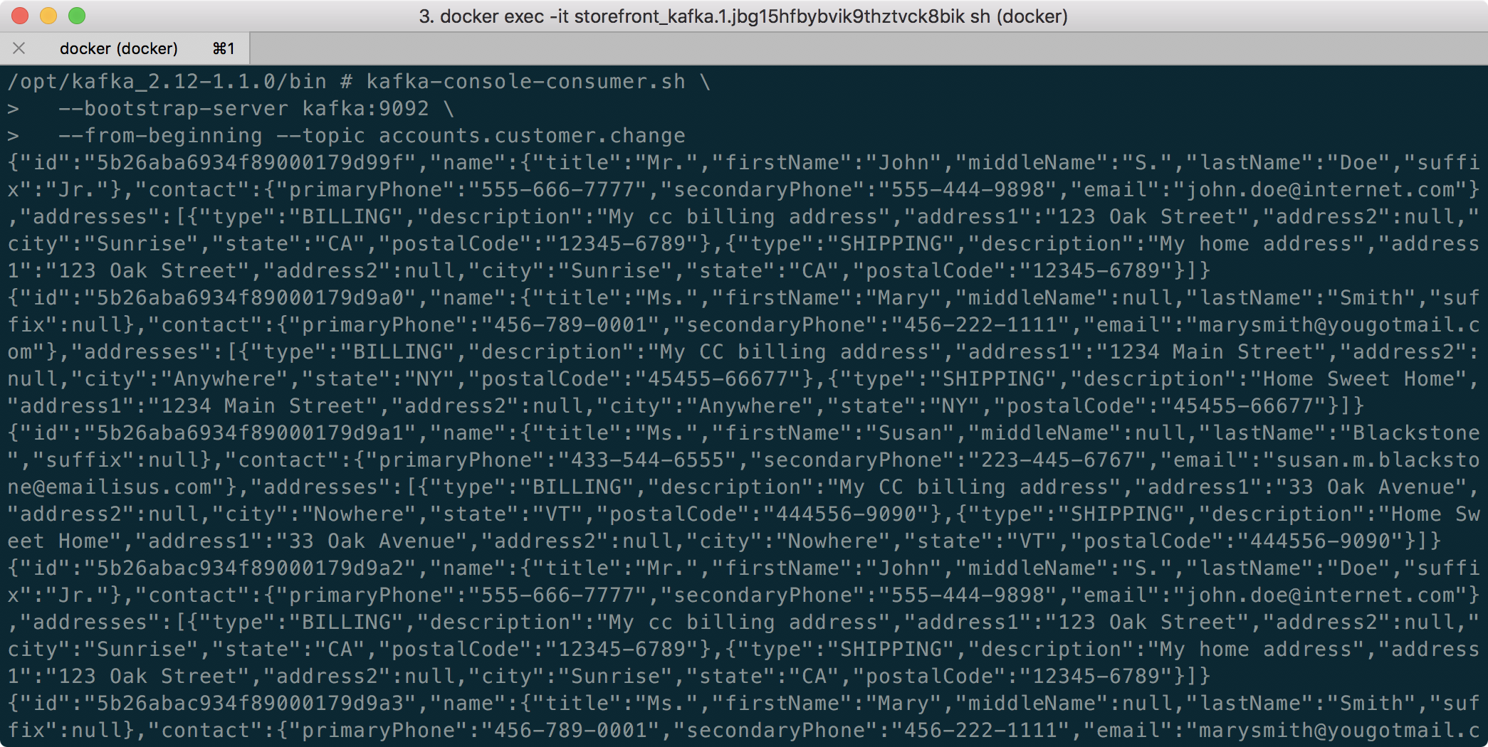
The Orders service’s Receiver class consumes the CustomerChangeEvent messages, produced by the Accounts service (gist).
[gust]cc3c4e55bc291e5435eccdd679d03015[/gist]
The Orders service’s Receiver class is configured differently, compared to the Fulfillment service. The Orders service receives messages from multiple topics, each containing messages with different payload structures. Each type of message must be deserialized into different object types. To accomplish this, the ReceiverConfig class uses Apache Kafka’s StringDeserializer. The Orders service’s ReceiverConfig references Spring Kafka’s AbstractKafkaListenerContainerFactory classes setMessageConverter method, which allows for dynamic object type matching (gist).
| @Configuration | |
| @EnableKafka | |
| public class ReceiverConfigNotConfluent implements ReceiverConfig { | |
| @Value("${spring.kafka.bootstrap-servers}") | |
| private String bootstrapServers; | |
| @Value("${spring.kafka.consumer.group-id}") | |
| private String groupId; | |
| @Value("${spring.kafka.consumer.auto-offset-reset}") | |
| private String autoOffsetReset; | |
| @Override | |
| @Bean | |
| public Map<String, Object> consumerConfigs() { | |
| Map<String, Object> props = new HashMap<>(); | |
| props.put(ProducerConfig.BOOTSTRAP_SERVERS_CONFIG, bootstrapServers); | |
| props.put(ConsumerConfig.KEY_DESERIALIZER_CLASS_CONFIG, StringDeserializer.class); | |
| props.put(ConsumerConfig.VALUE_DESERIALIZER_CLASS_CONFIG, StringDeserializer.class); | |
| props.put(ConsumerConfig.GROUP_ID_CONFIG, groupId); | |
| props.put(ConsumerConfig.AUTO_OFFSET_RESET_CONFIG, autoOffsetReset); | |
| return props; | |
| } | |
| @Override | |
| @Bean | |
| public ConsumerFactory<String, String> consumerFactory() { | |
| return new DefaultKafkaConsumerFactory<>(consumerConfigs(), | |
| new StringDeserializer(), | |
| new StringDeserializer() | |
| ); | |
| } | |
| @Bean | |
| ConcurrentKafkaListenerContainerFactory<String, String> kafkaListenerContainerFactory() { | |
| ConcurrentKafkaListenerContainerFactory<String, String> factory = | |
| new ConcurrentKafkaListenerContainerFactory<>(); | |
| factory.setConsumerFactory(consumerFactory()); | |
| factory.setMessageConverter(new StringJsonMessageConverter()); | |
| return factory; | |
| } | |
| @Override | |
| @Bean | |
| public Receiver receiver() { | |
| return new Receiver(); | |
| } | |
| } |
Each Kafka topic the Orders service consumes messages from is associated with a method in the Receiver class (shown above). That method accepts a specific object type as input, denoting the object type the message payload needs to be deserialized into. In this way, we can receive multiple message payloads, serialized from multiple object types, and successfully deserialize each type into the correct data object. In the case of a CustomerChangeEvent, the Orders service calls the receiveCustomerOrder method to consume the message and properly deserialize it.
For all services, a Spring application.yaml properties file, in each service’s resources directory, contains the Kafka configuration (gist).
| server: | |
| port: 8080 | |
| spring: | |
| main: | |
| allow-bean-definition-overriding: true | |
| application: | |
| name: orders | |
| data: | |
| mongodb: | |
| uri: mongodb://mongo:27017/orders | |
| kafka: | |
| bootstrap-servers: kafka:9092 | |
| topic: | |
| accounts-customer: accounts.customer.change | |
| orders-order: orders.order.fulfill | |
| fulfillment-order: fulfillment.order.change | |
| consumer: | |
| group-id: orders | |
| auto-offset-reset: earliest | |
| zipkin: | |
| sender: | |
| type: kafka | |
| management: | |
| endpoints: | |
| web: | |
| exposure: | |
| include: '*' | |
| logging: | |
| level: | |
| root: INFO | |
| --- | |
| spring: | |
| config: | |
| activate: | |
| on-profile: local | |
| data: | |
| mongodb: | |
| uri: mongodb://localhost:27017/orders | |
| kafka: | |
| bootstrap-servers: localhost:9092 | |
| server: | |
| port: 8090 | |
| management: | |
| endpoints: | |
| web: | |
| exposure: | |
| include: '*' | |
| logging: | |
| level: | |
| root: DEBUG | |
| --- | |
| spring: | |
| config: | |
| activate: | |
| on-profile: confluent | |
| server: | |
| port: 8080 | |
| logging: | |
| level: | |
| root: INFO | |
| --- | |
| server: | |
| port: 8080 | |
| spring: | |
| config: | |
| activate: | |
| on-profile: minikube | |
| data: | |
| mongodb: | |
| uri: mongodb://mongo.dev:27017/orders | |
| kafka: | |
| bootstrap-servers: kafka-cluster.dev:9092 | |
| management: | |
| endpoints: | |
| web: | |
| exposure: | |
| include: '*' | |
| logging: | |
| level: | |
| root: DEBUG |
Order Approved for Fulfillment
When the status of the Order in a CustomerOrders entity is changed to ‘Approved’ from ‘Created’, a FulfillmentRequestEvent message is produced and sent to the accounts.customer.change Kafka topic. This message is retrieved and consumed by the Fulfillment service. This is how the Fulfillment service has a record of what Orders are ready for fulfillment.

Since we did not create the Shopping Cart service for this post, the Orders service simulates an order approval event, containing an approved order, being received, through Kafka, from the Shopping Cart Service. To simulate order creation and approval, the Orders service can create a random order history for each customer. Further, the Orders service can scan all customer orders for orders that contain both a ‘Created’ and ‘Approved’ order status. This state is communicated as an event message to Kafka for all orders matching those criteria. A FulfillmentRequestEvent is produced, which contains the order to be fulfilled, and the customer’s contact and shipping information. The FulfillmentRequestEvent is passed to the Sender class (gist).
| @Slf4j | |
| public class Sender { | |
| @Autowired | |
| private KafkaTemplate<String, FulfillmentRequestEvent> kafkaTemplate; | |
| public void send(String topic, FulfillmentRequestEvent payload) { | |
| log.info("sending payload='{}' to topic='{}'", payload, topic); | |
| kafkaTemplate.send(topic, payload); | |
| } | |
| } |
The configuration of the Sender class is handled by the SenderConfig class. This Spring Kafka producer configuration class uses the Spring Kafka’s JsonSerializer class to serialize the FulfillmentRequestEvent object into a JSON message payload (gist).
| @Configuration | |
| @EnableKafka | |
| public class SenderConfig { | |
| @Value("${spring.kafka.bootstrap-servers}") | |
| private String bootstrapServers; | |
| @Bean | |
| public Map<String, Object> producerConfigs() { | |
| Map<String, Object> props = new HashMap<>(); | |
| props.put(ProducerConfig.BOOTSTRAP_SERVERS_CONFIG, bootstrapServers); | |
| props.put(ProducerConfig.KEY_SERIALIZER_CLASS_CONFIG, StringSerializer.class); | |
| props.put(ProducerConfig.VALUE_SERIALIZER_CLASS_CONFIG, JsonSerializer.class); | |
| return props; | |
| } | |
| @Bean | |
| public ProducerFactory<String, FulfillmentRequestEvent> producerFactory() { | |
| return new DefaultKafkaProducerFactory<>(producerConfigs()); | |
| } | |
| @Bean | |
| public KafkaTemplate<String, FulfillmentRequestEvent> kafkaTemplate() { | |
| return new KafkaTemplate<>(producerFactory()); | |
| } | |
| @Bean | |
| public Sender sender() { | |
| return new Sender(); | |
| } | |
| } |
The Sender class uses a KafkaTemplate to send the message to the Kafka topic, as shown below. Since message order is not critical messages could be sent to a topic with multiple partitions if the volume of messages required it.
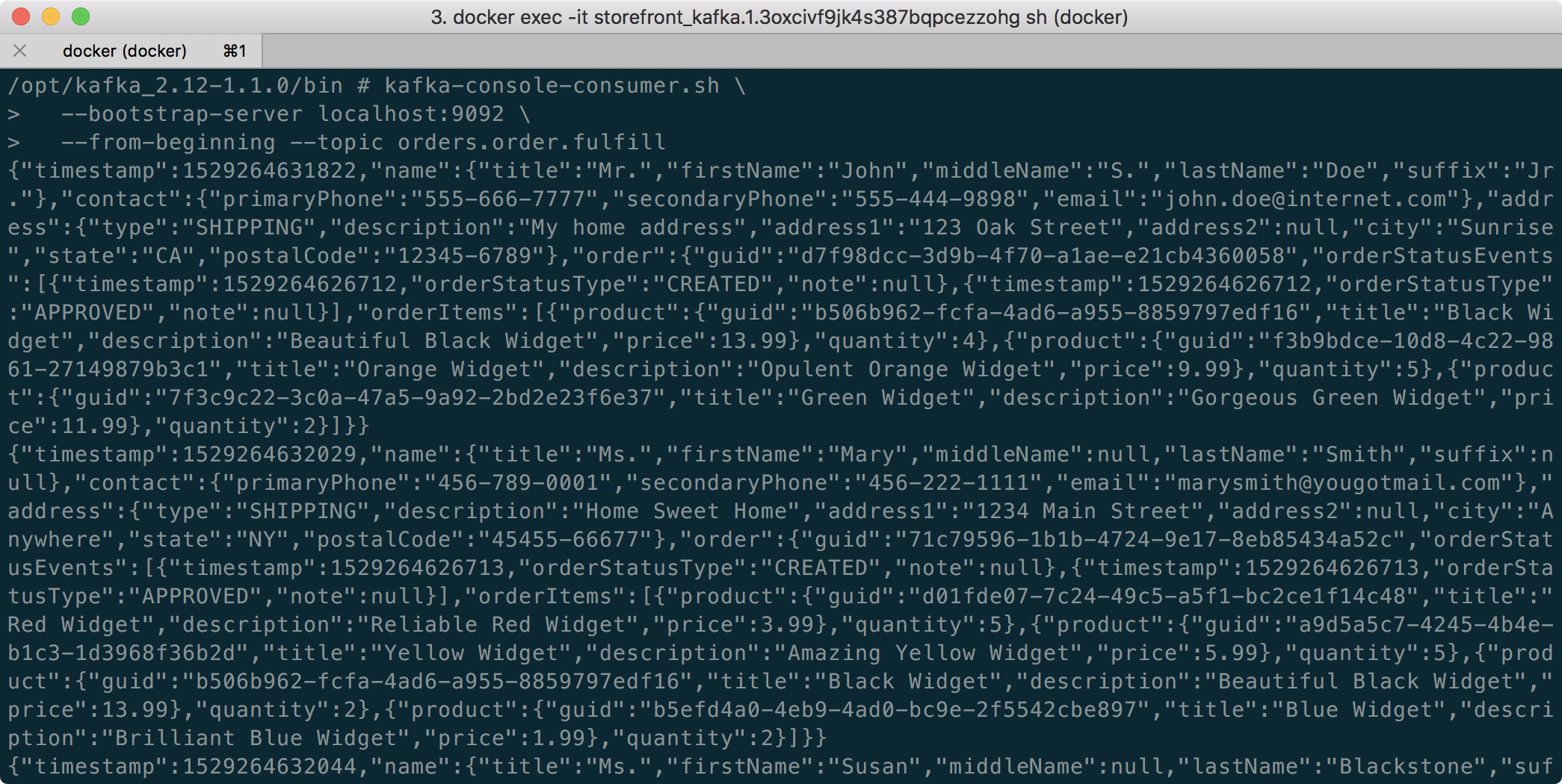
The Fulfillment service’s Receiver class consumes the FulfillmentRequestEvent from the Kafka topic and instantiates a Fulfillment object, containing the data passed in the FulfillmentRequestEvent message payload. This includes the order to be fulfilled and the customer’s contact and shipping information (gist).
| @Slf4j | |
| @Component | |
| public class Receiver { | |
| @Autowired | |
| private FulfillmentRepository fulfillmentRepository; | |
| private CountDownLatch latch = new CountDownLatch(1); | |
| public CountDownLatch getLatch() { | |
| return latch; | |
| } | |
| @KafkaListener(topics = "${spring.kafka.topic.orders-order}") | |
| public void receive(FulfillmentRequestEvent fulfillmentRequestEvent) { | |
| log.info("received payload='{}'", fulfillmentRequestEvent.toString()); | |
| latch.countDown(); | |
| Fulfillment fulfillment = new Fulfillment(); | |
| fulfillment.setId(fulfillmentRequestEvent.getId()); | |
| fulfillment.setTimestamp(fulfillmentRequestEvent.getTimestamp()); | |
| fulfillment.setName(fulfillmentRequestEvent.getName()); | |
| fulfillment.setContact(fulfillmentRequestEvent.getContact()); | |
| fulfillment.setAddress(fulfillmentRequestEvent.getAddress()); | |
| fulfillment.setOrder(fulfillmentRequestEvent.getOrder()); | |
| fulfillmentRepository.save(fulfillment); | |
| } | |
| } |
The Fulfillment service’s ReceiverConfig class defines the DefaultKafkaConsumerFactory and ConcurrentKafkaListenerContainerFactory, responsible for deserializing the message payload from JSON into a FulfillmentRequestEvent object (gist).
| @Configuration | |
| @EnableKafka | |
| public class ReceiverConfigNotConfluent implements ReceiverConfig { | |
| @Value("${spring.kafka.bootstrap-servers}") | |
| private String bootstrapServers; | |
| @Value("${spring.kafka.consumer.group-id}") | |
| private String groupId; | |
| @Value("${spring.kafka.consumer.auto-offset-reset}") | |
| private String autoOffsetReset; | |
| @Override | |
| @Bean | |
| public Map<String, Object> consumerConfigs() { | |
| Map<String, Object> props = new HashMap<>(); | |
| props.put(ConsumerConfig.BOOTSTRAP_SERVERS_CONFIG, bootstrapServers); | |
| props.put(ConsumerConfig.KEY_DESERIALIZER_CLASS_CONFIG, StringDeserializer.class); | |
| props.put(ConsumerConfig.VALUE_DESERIALIZER_CLASS_CONFIG, JsonDeserializer.class); | |
| props.put(ConsumerConfig.GROUP_ID_CONFIG, groupId); | |
| props.put(ConsumerConfig.AUTO_OFFSET_RESET_CONFIG, autoOffsetReset); | |
| return props; | |
| } | |
| @Override | |
| @Bean | |
| public ConsumerFactory<String, FulfillmentRequestEvent> consumerFactory() { | |
| return new DefaultKafkaConsumerFactory<>(consumerConfigs(), | |
| new StringDeserializer(), | |
| new JsonDeserializer<>(FulfillmentRequestEvent.class)); | |
| } | |
| @Override | |
| @Bean | |
| public ConcurrentKafkaListenerContainerFactory<String, FulfillmentRequestEvent> kafkaListenerContainerFactory() { | |
| ConcurrentKafkaListenerContainerFactory<String, FulfillmentRequestEvent> factory = | |
| new ConcurrentKafkaListenerContainerFactory<>(); | |
| factory.setConsumerFactory(consumerFactory()); | |
| return factory; | |
| } | |
| @Override | |
| @Bean | |
| public Receiver receiver() { | |
| return new Receiver(); | |
| } | |
| } |
Fulfillment Order Status State Change
When the status of the Order in a Fulfillment entity is changed to anything other than ‘Approved’, an OrderStatusChangeEvent message is produced by the Fulfillment service and sent to the fulfillment.order.change Kafka topic. This message is retrieved and consumed by the Orders service. This is how the Orders service tracks all CustomerOrder lifecycle events from the initial ‘Created’ status to the final happy path ‘Received’ status.

The Fulfillment service exposes several endpoints through the FulfillmentController class, which are simulate a change the status of an order. They allow an order status to be changed from ‘Approved’ to ‘Processing’, to ‘Shipped’, to ‘In Transit’, and to ‘Received’. This change is applied to all orders that meet the criteria.
Each of these state changes triggers a change to the Fulfillment document in MongoDB. Each change also generates an Kafka message, containing the OrderStatusChangeEvent in the message payload. This is handled by the Fulfillment service’s Sender class.
Note in this example, these two events are not handled in an atomic transaction. Either the updating the database or the sending of the message could fail independently, which would cause a loss of data consistency. In the real world, we must ensure both these disparate actions succeed or fail as a single transaction, to ensure data consistency (gist).
| @Slf4j | |
| public class Sender { | |
| @Autowired | |
| private KafkaTemplate<String, OrderStatusChangeEvent> kafkaTemplate; | |
| public void send(String topic, OrderStatusChangeEvent payload) { | |
| log.info("sending payload='{}' to topic='{}'", payload, topic); | |
| kafkaTemplate.send(topic, payload); | |
| } | |
| } |
The configuration of the Sender class is handled by the SenderConfig class. This Spring Kafka producer configuration class uses the Spring Kafka’s JsonSerializer class to serialize the OrderStatusChangeEvent object into a JSON message payload. This class is almost identical to the SenderConfig class in the Orders and Accounts services (gist).
| @Configuration | |
| @EnableKafka | |
| public class SenderConfig { | |
| @Value("${spring.kafka.bootstrap-servers}") | |
| private String bootstrapServers; | |
| @Bean | |
| public Map<String, Object> producerConfigs() { | |
| Map<String, Object> props = new HashMap<>(); | |
| props.put(ProducerConfig.BOOTSTRAP_SERVERS_CONFIG, bootstrapServers); | |
| props.put(ProducerConfig.KEY_SERIALIZER_CLASS_CONFIG, StringSerializer.class); | |
| props.put(ProducerConfig.VALUE_SERIALIZER_CLASS_CONFIG, JsonSerializer.class); | |
| return props; | |
| } | |
| @Bean | |
| public ProducerFactory<String, OrderStatusChangeEvent> producerFactory() { | |
| return new DefaultKafkaProducerFactory<>(producerConfigs()); | |
| } | |
| @Bean | |
| public KafkaTemplate<String, OrderStatusChangeEvent> kafkaTemplate() { | |
| return new KafkaTemplate<>(producerFactory()); | |
| } | |
| @Bean | |
| public Sender sender() { | |
| return new Sender(); | |
| } | |
| } |
The Sender class uses a KafkaTemplate to send the message to the Kafka topic, as shown below. Message order is not critical since a timestamp is recorded, which ensures the proper sequence of order status events can be maintained. Messages could be sent to a topic with multiple partitions if the volume of messages required it.

The Orders service’s Receiver class is responsible for consuming the OrderStatusChangeEvent message, produced by the Fulfillment service (gist).
| @Slf4j | |
| @Component | |
| public class Receiver { | |
| @Autowired | |
| private CustomerOrdersRepository customerOrdersRepository; | |
| @Autowired | |
| private MongoTemplate mongoTemplate; | |
| private CountDownLatch latch = new CountDownLatch(1); | |
| public CountDownLatch getLatch() { | |
| return latch; | |
| } | |
| @KafkaListener(topics = "${spring.kafka.topic.accounts-customer}") | |
| public void receiveCustomerOrder(CustomerOrders customerOrders) { | |
| log.info("received payload='{}'", customerOrders); | |
| latch.countDown(); | |
| customerOrdersRepository.save(customerOrders); | |
| } | |
| @KafkaListener(topics = "${spring.kafka.topic.fulfillment-order}") | |
| public void receiveOrderStatusChangeEvents(OrderStatusChangeEvent orderStatusChangeEvent) { | |
| log.info("received payload='{}'", orderStatusChangeEvent); | |
| latch.countDown(); | |
| Criteria criteria = Criteria.where("orders.guid") | |
| .is(orderStatusChangeEvent.getGuid()); | |
| Query query = Query.query(criteria); | |
| Update update = new Update(); | |
| update.addToSet("orders.$.orderStatusEvents", orderStatusChangeEvent.getOrderStatusEvent()); | |
| mongoTemplate.updateFirst(query, update, "customer.orders"); | |
| } | |
| } |
As explained above, the Orders service is configured differently compared to the Fulfillment service, to receive messages from Kafka. The Orders service needs to receive messages from more than one topic. The ReceiverConfig class deserializes all message using the StringDeserializer. The Orders service’s ReceiverConfig class references the Spring Kafka AbstractKafkaListenerContainerFactory classes setMessageConverter method, which allows for dynamic object type matching (gist).
| @Configuration | |
| @EnableKafka | |
| public class ReceiverConfigNotConfluent implements ReceiverConfig { | |
| @Value("${spring.kafka.bootstrap-servers}") | |
| private String bootstrapServers; | |
| @Value("${spring.kafka.consumer.group-id}") | |
| private String groupId; | |
| @Value("${spring.kafka.consumer.auto-offset-reset}") | |
| private String autoOffsetReset; | |
| @Override | |
| @Bean | |
| public Map<String, Object> consumerConfigs() { | |
| Map<String, Object> props = new HashMap<>(); | |
| props.put(ProducerConfig.BOOTSTRAP_SERVERS_CONFIG, bootstrapServers); | |
| props.put(ConsumerConfig.KEY_DESERIALIZER_CLASS_CONFIG, StringDeserializer.class); | |
| props.put(ConsumerConfig.VALUE_DESERIALIZER_CLASS_CONFIG, StringDeserializer.class); | |
| props.put(ConsumerConfig.GROUP_ID_CONFIG, groupId); | |
| props.put(ConsumerConfig.AUTO_OFFSET_RESET_CONFIG, autoOffsetReset); | |
| return props; | |
| } | |
| @Override | |
| @Bean | |
| public ConsumerFactory<String, String> consumerFactory() { | |
| return new DefaultKafkaConsumerFactory<>(consumerConfigs(), | |
| new StringDeserializer(), | |
| new StringDeserializer() | |
| ); | |
| } | |
| @Bean | |
| ConcurrentKafkaListenerContainerFactory<String, String> kafkaListenerContainerFactory() { | |
| ConcurrentKafkaListenerContainerFactory<String, String> factory = | |
| new ConcurrentKafkaListenerContainerFactory<>(); | |
| factory.setConsumerFactory(consumerFactory()); | |
| factory.setMessageConverter(new StringJsonMessageConverter()); | |
| return factory; | |
| } | |
| @Override | |
| @Bean | |
| public Receiver receiver() { | |
| return new Receiver(); | |
| } | |
| } |
Each Kafka topic the Orders service consumes messages from is associated with a method in the Receiver class (shown above). This method accepts a specific object type as an input parameter, denoting the object type the message payload needs to be deserialized into. In the case of an OrderStatusChangeEvent message, the receiveOrderStatusChangeEvents method is called to consume a message from the fulfillment.order.change Kafka topic.
Part Two
In Part Two of this post, I will briefly cover how to deploy and run a local development version of the storefront components, using Docker. The storefront’s microservices will be exposed through an API Gateway, Netflix’s Zuul. Service discovery and load balancing will be handled by Netflix’s Eureka. Both Zuul and Eureka are part of the Spring Cloud Netflix project. To provide operational visibility, we will add Yahoo’s Kafka Manager and Mongo Express to our system.
All opinions expressed in this post are my own and not necessarily the views of my current or past employers or their clients.
Developing Applications for the Cloud with Azure App Services and MongoDB Atlas
Posted by Gary A. Stafford in .NET Development, Azure, Cloud, Software Development on November 1, 2017
Shift Left Cloud
The continued growth of compute services by leading Cloud Service Providers (CSPs) like Microsoft, Amazon, and Google are transforming the architecture of modern software applications, as well as the software development lifecycle (SDLC). Self-service access to fully-managed, reasonably-priced, secure compute has significantly increased developer productivity. At the same time, cloud-based access to cutting-edge technologies, like Artificial Intelligence (AI), Internet Of Things (IoT), Machine Learning, and Data Analytics, has accelerated the capabilities of modern applications. Finally, as CSPs become increasingly platform agnostic, Developers are no longer limited to a single technology stack or operating system. Today, Developers are solving complex problems with multi-cloud, multi-OS polyglot solutions.
Developers now leverage the Cloud from the very start of the software development process; shift left Cloud, if you will*. Developers are no longer limited to building and testing software on local workstations or on-premise servers, then throwing it over the wall to Operations for deployment to the Cloud. Developers using Azure, AWS, and GCP, develop, build, test, and deploy their code directly to the Cloud. Existing organizations are rapidly moving development environments from on-premise to the Cloud. New organizations are born in the Cloud, without the burden of legacy on-premise data-centers and servers under desks to manage.
Example Application
To demonstrate the ease of developing a modern application for the Cloud, let’s explore a simple API-based, NoSQL-backed web application. The application, The .NET Diner, simulates a rudimentary restaurant menu ordering interface. It consists of a single-page application (SPA) and two microservices backed by MongoDB. For simplicity, there is no API Gateway between the UI and the two services, as normally would be in place. An earlier version of this application was used in two previous posts, including Cloud-based Continuous Integration and Deployment for .NET Development.
The original restaurant order application was written with JQuery and RESTful .NET WCF Services. The new application, used in this post, has been completely re-written and modernized. The web-based user interface (UI) is written with Google’s Angular 4 framework using TypeScript. The UI relies on a microservices-based API, built with C# using Microsoft’s Web API 2 and .NET 4.7. The services rely on MongoDB for data persistence.

All code for this project is available on GitHub within two projects, one for the Angular UI and another for the C# services. The entire application can easily be built and run locally on Windows using MongoDB Community Edition. Alternately, to run the application in the Cloud, you will require an Azure and MongoDB Atlas account.
This post is primarily about the development experience. For brevity, the post will not delve into security, DevOps practices for CI/CD, and the complexities of staging and releasing code to Production.
Cross-Platform Development
The API, consisting of a set of C# microservices, was developed with Microsoft Visual Studio Community 2017 on Windows 10. Visual Studio touts itself as a full-featured Integrated Development Environment (IDE) for Android, iOS, Windows, web, and cloud. Visual Studio is easily integrated with Azure, AWS, and Google, through the use of Extensions. Visual Studio is an ideal IDE for cloud-centric application development.

To simulate a typical mixed-platform development environment, the Angular UI front-end was developed with JetBrains WebStorm 2017 on Mac OS X. WebStorm touts itself as a powerful IDE for modern JavaScript development.

Other tools used to develop the application include Git and GitHub for source code, MongoDB Community Edition for local database development, and Postman for API development and testing, both locally and on Azure. All the development tools used in the post are cross-platform. Versions of WebStorm, Visual Studio, MongoDB, Postman, Git, Node.js, npm, and Bash are all available for Mac, Windows, and Linux. Cross-platform flexibility is key when developing modern multi-OS polyglot applications.
Postman
Postman was used to build, test, and document the application’s API. Postman is an excellent choice for developing RESTful APIs. With Postman, you define Collections of HTTP requests for each of your APIs. You then define Environments, such as Development, Test, and Production, against which you will execute the Collections of HTTP requests. Each environment consists of environment-specific variables. Those variables can be used to define API URLs and as request parameters.
Not only can you define static variables, Postman’s runtime, built on Node.js, is scriptable using JavaScript, allowing you to programmatically set dynamic variables, based on the results of HTTP requests and responses, as demonstrated below.

Postman also allows you to write and run automated API integration tests, as well as perform load testing, as shown below.

Azure App Services
The Angular browser-based UI and the C# microservices will be deployed to Azure using the Azure App Service. Azure App Service is nearly identical to AWS Elastic BeanStalk and Google App Engine. According to Microsoft, Azure App Service allows Developers to quickly build, deploy, and scale enterprise-grade web, mobile, and API apps, running on Windows or Linux, using .NET, .NET Core, Java, Ruby, Node.js, PHP, and Python.
App Service is a fully-managed, turn-key platform. Azure takes care of infrastructure maintenance and load balancing. App Service easily integrates with other Azure services, such as API Management, Queue Storage, Azure Active Directory (AD), Cosmos DB, and Application Insights. Microsoft suggests evaluating the following four criteria when considering Azure App Services:
- You want to deploy a web application that’s accessible through the Internet.
- You want to automatically scale your web application according to demand without needing to redeploy.
- You don’t want to maintain server infrastructure (including software updates).
- You don’t need any machine-level customizations on the servers that host your web application.
There are currently four types of Azure App Services, which are Web Apps, Web Apps for Containers, Mobile Apps, and API Apps. The application in this post will use the Azure Web Apps for the Angular browser-based UI and Azure API Apps for the C# microservices.
MongoDB Atlas
Each of the C# microservices has separate MongoDB database. In the Cloud, the services use MongoDB Atlas, a secure, highly-available, and scalable cloud-hosted MongoDB service. Cloud-based databases, like Atlas, are often referred to as Database as a Service (DBaaS). Atlas is a Cloud-based alternative to traditional on-premise databases, as well as equivalent CSP-based solutions, such as Amazon DynamoDB, GCP Cloud Bigtable, and Azure Cosmos DB.
Atlas is an example of a SaaS who offer a single service or small set of closely related services, as an alternative to the big CSP’s equivalent services. Similar providers in this category include CloudAMQP (RabbitMQ as a Service), ClearDB (MySQL DBaaS), Akamai (Content Delivery Network), and Oracle Database Cloud Service (Oracle Database, RAC, and Exadata as a Service). Many of these providers, such as Atlas, are themselves hosted on AWS or other CSPs.
There are three pricing levels for MongoDB Atlas: Free, Essential, and Professional. To follow along with this post, the Free level is sufficient. According to MongoDB, with the Free account level, you get 512 MB of storage with shared RAM, a highly-available 3-node replica set, end-to-end encryption, secure authentication, fully managed upgrades, monitoring and alerts, and a management API. Atlas provides the ability to upgrade your account and CSP specifics at any time.
Once you register for an Atlas account, you will be able to log into Atlas, set up your users, whitelist your IP addresses for security, and obtain necessary connection information. You will need this connection information in the next section to configure the Azure API Apps.

With the Free Atlas tier, you can view detailed Metrics about database cluster activity. However, with the free tier, you do not get access to Real-Time data insights or the ability to use the Data Explorer to view your data through the Atlas UI.

Azure API Apps
The example application’s API consists of two RESTful microservices built with C#, the RestaurantMenu service and RestaurantOrder service. Both services are deployed as Azure API Apps. API Apps is a fully-managed platform. Azure performs OS patching, capacity provisioning, server management, and load balancing.
Microsoft Visual Studio has done an excellent job providing Extensions to make cloud integration a breeze. I will be using Visual Studio Tools for Azure in this post. Similar to how you create a Publish Profile for deploying applications to Internet Information Services (IIS), you create a Publish Profile for Azure App Services. Using the step-by-step user interface, you create a Microsft Azure App Service Web Deploy Publish Profile for each service. To create a new Profile, choose the Microsoft Azure App Service Target.

You must be connected to your Azure account to create the Publish Profile. Give the service an App Name, choose your Subscription, and select or create a Resource Group and an App Service Plan.

The App Service Plan defines the Location and Size for your API App container; these will determine the cost of the compute. I suggest putting the two API Apps and the Web App in the same location, in this case, East US.

The Publish Profile is now available for deploying the services to Azure. No command line interaction is required. The services can be built and published to Azure with a single click from within Visual Studio.

Configuration Management
Azure App Services is highly configurable. For example, each API App requires a different configuration, in each environment, to connect to different instances of MongoDB Atlas databases. For security, sensitive Atlas credentials are not stored in the source code. The Atlas URL and sensitive credentials are stored in App Settings on Azure. For this post, the settings were input directly into the Azure UI, as shown below. You will need to input your own Atlas URL and credentials.
The compiled C# services expect certain environment variables to be present at runtime to connect to MongoDB Atlas. These are provided through Azure’s App Settings. Access to the App Settings in Azure should be tightly controlled through Azure AD and fine-grained Azure Role-Based Access Control (RBAC) service.

CORS
If you want to deploy the application from this post to Azure, there is one code change you will need to make to each service, which deals with Cross-Origin Resource Sharing (CORS). The services are currently configured to only accept traffic from my temporary Angular UI App Service’s URL. You will need to adjust the CORS configuration in the \App_Start\WebApiConfig.cs file in each service, to match your own App Service’s new URL.
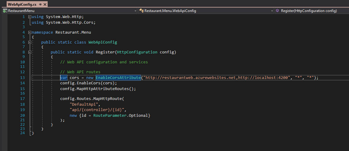
Angular UI Web App
The Angular UI application will be deployed as an Azure Web App, one of four types of Azure App Services, mentioned previously. According to Microsoft, Web Apps allow Developers to program in their favorite languages, including .NET, Java, Node.js, PHP, and Python on Windows or .NET Core, Node.js, PHP or Ruby on Linux. Web Apps is a fully-managed platform. Azure performs OS patching, capacity provisioning, server management, and load balancing.
Using the Azure Portal, setting up a new Web App for the Angular UI is simple.

Provide an App Name, Subscription, Resource Group, OS Type, and select whether or not you want Application Insights enabled for the Web App.

Although an amazing IDE for web development, WebStorm lacks some of the direct integrations with Azure, AWS, and Google, available with other IDE’s, like Visual Studio. Since the Angular application was developed in WebStorm on Mac, we will take advantage of Azure App Service’s Continuous Deployment feature.
Azure Web Apps can be deployed automatically from most common source code management platforms, including Visual Studio Team Services (VSTS), GitHub, Bitbucket, OneDrive, and local Git repositories.

For this post, I chose GitHub. To configure deployment from GitHub, select the GitHub Account, Organization, Project, and Branch from which Azure will deploy the Angular Web App.

Configuring GitHub in the Azure Portal, Azure becomes an Authorized OAuth App on the GitHub account. Azure creates a Webhook, which fires each time files are pushed (git push) to the dist branch of the GitHub project’s repository.

Using the ng build --dev --env=prod command, the Angular UI application must be first transpiled from TypeScript to JavaScript and bundled for deployment. The ng build command can be run from within WebStorm or from the command line.

The the --env=prod flag ensures that the Production environment configuration, containing the correct Azure API endpoints, issued transpiled into the build. This configuration is stored in the \src\environments\environment.prod.ts file, shown below. You will need to update these two endpoints to your own endpoints from the two API Apps you previously deployed to Azure.

Optionally, the code should be optimized for Production, by replacing the --dev flag with the --prod flag. Amongst other optimizations, the Production version of the code is uglified using UglifyJS. Note the difference in the build files shown below for Production, as compared to files above for Development.

Since I chose GitHub for deployment to Azure, I used Git to manually push the local build files to the dist branch on GitHub.

Every time the webhook fires, Azure pulls and deploys the new build, overwriting the previously deployed version, as shown below.

To stage new code and not immediately overwrite running code, Azure has a feature called Deployment slots. According to Microsoft, Deployment slots allow Developers to deploy different versions of Web Apps to different URLs. You can test a certain version and then swap content and configuration between slots. This is likely how you would eventually deploy your code to Production.
Up and Running
Below, the three Azure App Services are shown in the Azure Portal, successfully deployed and running. Note their Status, App Type, Location, and Subscription.

Before exploring the deployed UI, the two Azure API Apps should be tested using Postman. Once the API is confirmed to be working properly, populated by making an HTTP Post request to the menuitems API, the RestaurantOrderService Azure API Service. When the HTTP Post request is made, the RestaurantOrderService stores a set of menu items in the RestaurantMenu Atlas MongoDB database, in the menus collection.

The Angular UI, the RestaurantWeb Azure Web App, is viewed by using the URL provided in the Web App’s Overview tab. The menu items displayed in the drop-down are supplied by an HTTP GET request to the menuitems API, provided by the RestaurantMenuService Azure API Service.

Your order is placed through an HTTP Post request to the orders API, the RestaurantOrderService Azure API Service. The RestaurantOrderService stores the order in the RestaurantOrder Atlas MongoDB database, in the orders collection. The order details are returned in the response body and displayed in the UI.

Once you have the development version of the application successfully up and running on Atlas and Azure, you can start to configure, test, and deploy additional application versions, as App Services, into higher Azure environments, such as Test, Performance, and eventually, Production.
Monitoring
Azure provides in-depth monitoring and performance analytics capabilities for your deployed applications with services like Application Insights. With Azure’s monitoring resources, you can monitor the live performance of your application and set up alerts for application errors and performance issues. Real-time monitoring useful when conducting performance tests. Developers can analyze response time of each API method and optimize the application, Azure configuration, and MongoDB databases, before deploying to Production.

Conclusion
This post demonstrated how the Cloud has shifted application development to a Cloud-first model. Future posts will demonstrate how an application, such as the app featured in this post, is secured, and how it is continuously built, tested, and deployed, using DevOps practices.
All opinions in this post are my own, and not necessarily the views of my current or past employers or their clients.
Spring Music Revisited: Java-Spring-MongoDB Web App with Docker 1.12
Posted by Gary A. Stafford in Build Automation, Continuous Delivery, DevOps, Enterprise Software Development, Java Development, Software Development on August 7, 2016
Build, test, deploy, and monitor a multi-container, MongoDB-backed, Java Spring web application, using the new Docker 1.12.
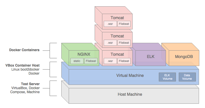
Introduction
This post and the post’s example project represent an update to a previous post, Build and Deploy a Java-Spring-MongoDB Application using Docker. This new post incorporates many improvements made in Docker 1.12, including the use of the new Docker Compose v2 YAML format. The post’s project was also updated to use Filebeat with ELK, as opposed to Logspout, which was used previously.
In this post, we will demonstrate how to build, test, deploy, and manage a Java Spring web application, hosted on Apache Tomcat, load-balanced by NGINX, monitored by ELK with Filebeat, and all containerized with Docker.
We will use a sample Java Spring application, Spring Music, available on GitHub from Cloud Foundry. The Spring Music sample record album collection application was originally designed to demonstrate the use of database services on Cloud Foundry, using the Spring Framework. Instead of Cloud Foundry, we will host the Spring Music application locally, using Docker on VirtualBox, and optionally on AWS.
All files necessary to build this project are stored on the docker_v2 branch of the garystafford/spring-music-docker repository on GitHub. The Spring Music source code is stored on the springmusic_v2 branch of the garystafford/spring-music repository, also on GitHub.

Application Architecture
The Java Spring Music application stack contains the following technologies: Java, Spring Framework, AngularJS, Bootstrap, jQuery, NGINX, Apache Tomcat, MongoDB, the ELK Stack, and Filebeat. Testing frameworks include the Spring MVC Test Framework, Mockito, Hamcrest, and JUnit.
A few changes were made to the original Spring Music application to make it work for this demonstration, including:
- Move from Java 1.7 to 1.8 (including newer Tomcat version)
- Add unit tests for Continuous Integration demonstration purposes
- Modify MongoDB configuration class to work with non-local, containerized MongoDB instances
- Add Gradle
warNoStatictask to build WAR without static assets - Add Gradle
zipStatictask to ZIP up the application’s static assets for deployment to NGINX - Add Gradle
zipGetVersiontask with a versioning scheme for build artifacts - Add
context.xmlfile andMANIFEST.MFfile to the WAR file - Add Log4j
RollingFileAppenderappender to send log entries to Filebeat - Update versions of several dependencies, including Gradle, Spring, and Tomcat
We will use the following technologies to build, publish, deploy, and host the Java Spring Music application: Gradle, git, GitHub, Travis CI, Oracle VirtualBox, Docker, Docker Compose, Docker Machine, Docker Hub, and optionally, Amazon Web Services (AWS).
NGINX
To increase performance, the Spring Music web application’s static content will be hosted by NGINX. The application’s WAR file will be hosted by Apache Tomcat 8.5.4. Requests for non-static content will be proxied through NGINX on the front-end, to a set of three load-balanced Tomcat instances on the back-end. To further increase application performance, NGINX will also be configured for browser caching of the static content. In many enterprise environments, the use of a Java EE application server, like Tomcat, is still not uncommon.
Reverse proxying and caching are configured thought NGINX’s default.conf file, in the server configuration section:
| server { | |
| listen 80; | |
| server_name proxy; | |
| location ~* \/assets\/(css|images|js|template)\/* { | |
| root /usr/share/nginx/; | |
| expires max; | |
| add_header Pragma public; | |
| add_header Cache-Control "public, must-revalidate, proxy-revalidate"; | |
| add_header Vary Accept-Encoding; | |
| access_log off; | |
| } |
The three Tomcat instances will be manually configured for load-balancing using NGINX’s default round-robin load-balancing algorithm. This is configured through the default.conf file, in the upstream configuration section:
| upstream backend { | |
| server music_app_1:8080; | |
| server music_app_2:8080; | |
| server music_app_3:8080; | |
| } |
Client requests are received through port 80 on the NGINX server. NGINX redirects requests, which are not for non-static assets, to one of the three Tomcat instances on port 8080.
MongoDB
The Spring Music application was designed to work with a number of data stores, including MySQL, Postgres, Oracle, MongoDB, Redis, and H2, an in-memory Java SQL database. Given the choice of both SQL and NoSQL databases, we will select MongoDB.
The Spring Music application, hosted by Tomcat, will store and modify record album data in a single instance of MongoDB. MongoDB will be populated with a collection of album data from a JSON file, when the Spring Music application first creates the MongoDB database instance.
ELK
Lastly, the ELK Stack with Filebeat, will aggregate NGINX, Tomcat, and Java Log4j log entries, providing debugging and analytics to our demonstration. A similar method for aggregating logs, using Logspout instead of Filebeat, can be found in this previous post.
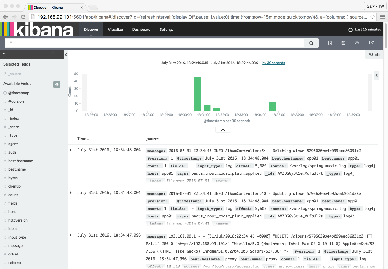
Continuous Integration
In this post’s example, two build artifacts, a WAR file for the application and ZIP file for the static web content, are built automatically by Travis CI, whenever source code changes are pushed to the springmusic_v2 branch of the garystafford/spring-music repository on GitHub.

Following a successful build and a small number of unit tests, Travis CI pushes the build artifacts to the build-artifacts branch on the same GitHub project. The build-artifacts branch acts as a pseudo binary repository for the project, much like JFrog’s Artifactory. These artifacts are used later by Docker to build the project’s immutable Docker images and containers.
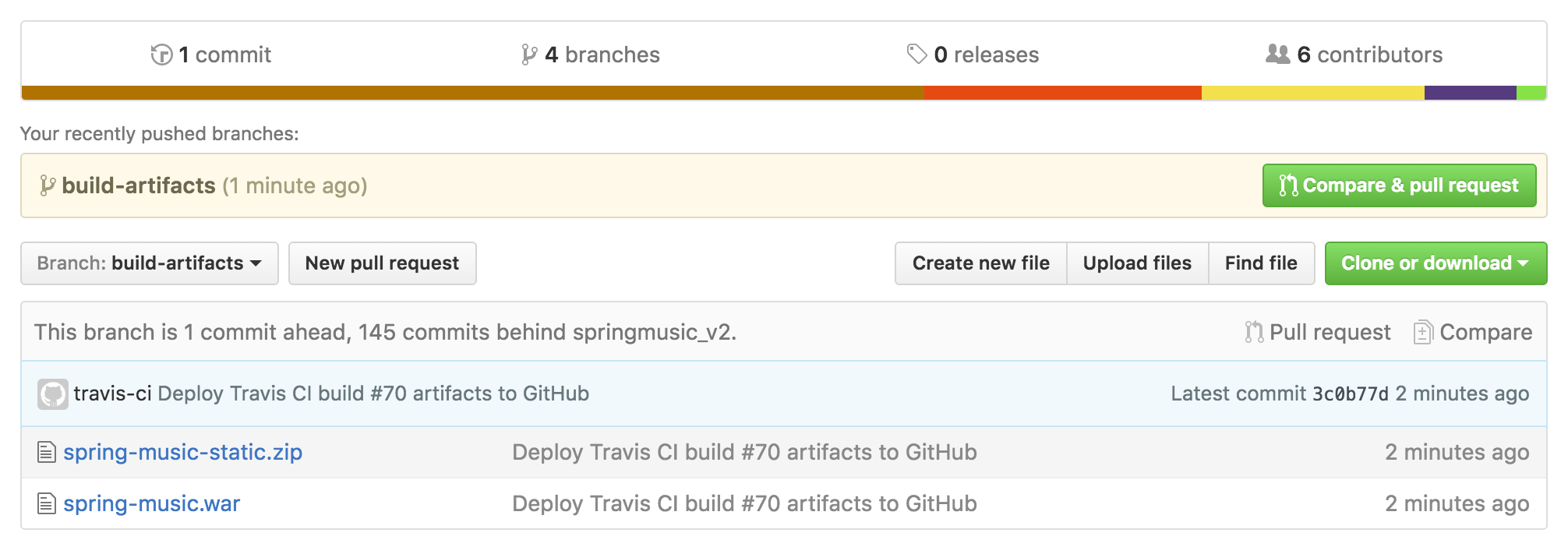
Build Notifications
Travis CI pushes build notifications to a Slack channel, which eliminates the need to actively monitor Travis CI.
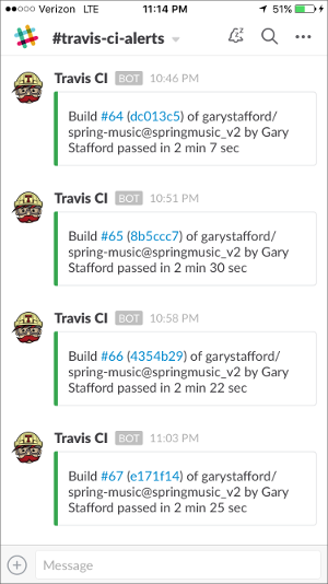
Automation Scripting
The .travis.yaml file, custom gradle.build Gradle tasks, and the deploy_travisci.sh script handles the Travis CI automation described, above.
Travis CI .travis.yaml file:
| language: java | |
| jdk: oraclejdk8 | |
| before_install: | |
| - chmod +x gradlew | |
| before_deploy: | |
| - chmod ugo+x deploy_travisci.sh | |
| script: | |
| - "./gradlew clean build" | |
| - "./gradlew warNoStatic warCopy zipGetVersion zipStatic" | |
| - sh ./deploy_travisci.sh | |
| env: | |
| global: | |
| - GH_REF: github.com/garystafford/spring-music.git | |
| - secure: <GH_TOKEN_secure_hash_here> | |
| - secure: <COMMIT_AUTHOR_EMAIL_secure_hash_here> | |
| notifications: | |
| slack: | |
| - secure: <SLACK_secure_hash_here> |
Custom gradle.build tasks:
| // new Gradle build tasks | |
| task warNoStatic(type: War) { | |
| // omit the version from the war file name | |
| version = '' | |
| exclude '**/assets/**' | |
| manifest { | |
| attributes | |
| 'Manifest-Version': '1.0', | |
| 'Created-By': currentJvm, | |
| 'Gradle-Version': GradleVersion.current().getVersion(), | |
| 'Implementation-Title': archivesBaseName + '.war', | |
| 'Implementation-Version': artifact_version, | |
| 'Implementation-Vendor': 'Gary A. Stafford' | |
| } | |
| } | |
| task warCopy(type: Copy) { | |
| from 'build/libs' | |
| into 'build/distributions' | |
| include '**/*.war' | |
| } | |
| task zipGetVersion (type: Task) { | |
| ext.versionfile = | |
| new File("${projectDir}/src/main/webapp/assets/buildinfo.properties") | |
| versionfile.text = 'build.version=' + artifact_version | |
| } | |
| task zipStatic(type: Zip) { | |
| from 'src/main/webapp/assets' | |
| appendix = 'static' | |
| version = '' | |
| } |
The deploy.sh file:
| #!/bin/bash | |
| set -e | |
| cd build/distributions | |
| git init | |
| git config user.name "travis-ci" | |
| git config user.email "${COMMIT_AUTHOR_EMAIL}" | |
| git add . | |
| git commit -m "Deploy Travis CI Build #${TRAVIS_BUILD_NUMBER} artifacts to GitHub" | |
| git push --force --quiet "https://${GH_TOKEN}@${GH_REF}" master:build-artifacts > /dev/null 2>&1 |
You can easily replicate the project’s continuous integration automation using your choice of toolchains. GitHub or BitBucket are good choices for distributed version control. For continuous integration and deployment, I recommend Travis CI, Semaphore, Codeship, or Jenkins. Couple those with a good persistent chat application, such as Glider Labs’ Slack or Atlassian’s HipChat.
Building the Docker Environment
Make sure VirtualBox, Docker, Docker Compose, and Docker Machine, are installed and running. At the time of this post, I have the following versions of software installed on my Mac:
- Mac OS X 10.11.6
- VirtualBox 5.0.26
- Docker 1.12.1
- Docker Compose 1.8.0
- Docker Machine 0.8.1
To build the project’s VirtualBox VM, Docker images, and Docker containers, execute the build script, using the following command: sh ./build_project.sh. A build script is useful when working with CI/CD automation tools, such as Jenkins CI or ThoughtWorks go. However, to understand the build process, I suggest first running the individual commands, locally.
| #!/bin/sh | |
| set -ex | |
| # clone project | |
| git clone -b docker_v2 --single-branch \ | |
| https://github.com/garystafford/spring-music-docker.git music \ | |
| && cd "$_" | |
| # provision VirtualBox VM | |
| docker-machine create --driver virtualbox springmusic | |
| # set new environment | |
| docker-machine env springmusic \ | |
| && eval "$(docker-machine env springmusic)" | |
| # mount a named volume on host to store mongo and elk data | |
| # ** assumes your project folder is 'music' ** | |
| docker volume create --name music_data | |
| docker volume create --name music_elk | |
| # create bridge network for project | |
| # ** assumes your project folder is 'music' ** | |
| docker network create -d bridge music_net | |
| # build images and orchestrate start-up of containers (in this order) | |
| docker-compose -p music up -d elk && sleep 15 \ | |
| && docker-compose -p music up -d mongodb && sleep 15 \ | |
| && docker-compose -p music up -d app \ | |
| && docker-compose scale app=3 && sleep 15 \ | |
| && docker-compose -p music up -d proxy && sleep 15 | |
| # optional: configure local DNS resolution for application URL | |
| #echo "$(docker-machine ip springmusic) springmusic.com" | sudo tee --append /etc/hosts | |
| # run a simple connectivity test of application | |
| for i in {1..9}; do curl -I $(docker-machine ip springmusic); done |
Deploying to AWS
By simply changing the Docker Machine driver to AWS EC2 from VirtualBox, and providing your AWS credentials, the springmusic environment may also be built on AWS.
Build Process
Docker Machine provisions a single VirtualBox springmusic VM on which host the project’s containers. VirtualBox provides a quick and easy solution that can be run locally for initial development and testing of the application.
Next, the script creates a Docker data volume and project-specific Docker bridge network.
Next, using the project’s individual Dockerfiles, Docker Compose pulls base Docker images from Docker Hub for NGINX, Tomcat, ELK, and MongoDB. Project-specific immutable Docker images are then built for NGINX, Tomcat, and MongoDB. While constructing the project-specific Docker images for NGINX and Tomcat, the latest Spring Music build artifacts are pulled and installed into the corresponding Docker images.
Docker Compose builds and deploys (6) containers onto the VirtualBox VM: (1) NGINX, (3) Tomcat, (1) MongoDB, and (1) ELK.
The NGINX Dockerfile:
| # NGINX image with build artifact | |
| FROM nginx:latest | |
| MAINTAINER Gary A. Stafford <garystafford@rochester.rr.com> | |
| ENV REFRESHED_AT 2016-09-17 | |
| ENV GITHUB_REPO https://github.com/garystafford/spring-music/raw/build-artifacts | |
| ENV STATIC_FILE spring-music-static.zip | |
| RUN apt-get update -qq \ | |
| && apt-get install -qqy curl wget unzip nano \ | |
| && apt-get clean \ | |
| \ | |
| && wget -O /tmp/${STATIC_FILE} ${GITHUB_REPO}/${STATIC_FILE} \ | |
| && unzip /tmp/${STATIC_FILE} -d /usr/share/nginx/assets/ | |
| COPY default.conf /etc/nginx/conf.d/default.conf | |
| # tweak nginx image set-up, remove log symlinks | |
| RUN rm /var/log/nginx/access.log /var/log/nginx/error.log | |
| # install Filebeat | |
| ENV FILEBEAT_VERSION=filebeat_1.2.3_amd64.deb | |
| RUN curl -L -O https://download.elastic.co/beats/filebeat/${FILEBEAT_VERSION} \ | |
| && dpkg -i ${FILEBEAT_VERSION} \ | |
| && rm ${FILEBEAT_VERSION} | |
| # configure Filebeat | |
| ADD filebeat.yml /etc/filebeat/filebeat.yml | |
| # CA cert | |
| RUN mkdir -p /etc/pki/tls/certs | |
| ADD logstash-beats.crt /etc/pki/tls/certs/logstash-beats.crt | |
| # start Filebeat | |
| ADD ./start.sh /usr/local/bin/start.sh | |
| RUN chmod +x /usr/local/bin/start.sh | |
| CMD [ "/usr/local/bin/start.sh" ] |
The Tomcat Dockerfile:
| # Apache Tomcat image with build artifact | |
| FROM tomcat:8.5.4-jre8 | |
| MAINTAINER Gary A. Stafford <garystafford@rochester.rr.com> | |
| ENV REFRESHED_AT 2016-09-17 | |
| ENV GITHUB_REPO https://github.com/garystafford/spring-music/raw/build-artifacts | |
| ENV APP_FILE spring-music.war | |
| ENV TERM xterm | |
| ENV JAVA_OPTS -Djava.security.egd=file:/dev/./urandom | |
| RUN apt-get update -qq \ | |
| && apt-get install -qqy curl wget \ | |
| && apt-get clean \ | |
| \ | |
| && touch /var/log/spring-music.log \ | |
| && chmod 666 /var/log/spring-music.log \ | |
| \ | |
| && wget -q -O /usr/local/tomcat/webapps/ROOT.war ${GITHUB_REPO}/${APP_FILE} \ | |
| && mv /usr/local/tomcat/webapps/ROOT /usr/local/tomcat/webapps/_ROOT | |
| COPY tomcat-users.xml /usr/local/tomcat/conf/tomcat-users.xml | |
| # install Filebeat | |
| ENV FILEBEAT_VERSION=filebeat_1.2.3_amd64.deb | |
| RUN curl -L -O https://download.elastic.co/beats/filebeat/${FILEBEAT_VERSION} \ | |
| && dpkg -i ${FILEBEAT_VERSION} \ | |
| && rm ${FILEBEAT_VERSION} | |
| # configure Filebeat | |
| ADD filebeat.yml /etc/filebeat/filebeat.yml | |
| # CA cert | |
| RUN mkdir -p /etc/pki/tls/certs | |
| ADD logstash-beats.crt /etc/pki/tls/certs/logstash-beats.crt | |
| # start Filebeat | |
| ADD ./start.sh /usr/local/bin/start.sh | |
| RUN chmod +x /usr/local/bin/start.sh | |
| CMD [ "/usr/local/bin/start.sh" ] |
Docker Compose v2 YAML
This post was recently updated for Docker 1.12, and to use Docker Compose v2 YAML file format. The post’s docker-compose.yml takes advantage of improvements in Docker 1.12 and Docker Compose v2 YAML. Improvements to the YAML file include eliminating the need to link containers and expose ports, and the addition of named networks and volumes.
| version: '2' | |
| services: | |
| proxy: | |
| build: nginx/ | |
| ports: | |
| - 80:80 | |
| networks: | |
| - net | |
| depends_on: | |
| - app | |
| hostname: proxy | |
| container_name: proxy | |
| app: | |
| build: tomcat/ | |
| ports: | |
| - 8080 | |
| networks: | |
| - net | |
| depends_on: | |
| - mongodb | |
| hostname: app | |
| mongodb: | |
| build: mongodb/ | |
| ports: | |
| - 27017:27017 | |
| networks: | |
| - net | |
| depends_on: | |
| - elk | |
| hostname: mongodb | |
| container_name: mongodb | |
| volumes: | |
| - music_data:/data/db | |
| - music_data:/data/configdb | |
| elk: | |
| image: sebp/elk:latest | |
| ports: | |
| - 5601:5601 | |
| - 9200:9200 | |
| - 5044:5044 | |
| - 5000:5000 | |
| networks: | |
| - net | |
| volumes: | |
| - music_elk:/var/lib/elasticsearch | |
| hostname: elk | |
| container_name: elk | |
| volumes: | |
| music_data: | |
| external: true | |
| music_elk: | |
| external: true | |
| networks: | |
| net: | |
| driver: bridge |
The Results
Below are the results of building the project.
| # Resulting Docker Machine VirtualBox VM: | |
| $ docker-machine ls | |
| NAME ACTIVE DRIVER STATE URL SWARM DOCKER ERRORS | |
| springmusic * virtualbox Running tcp://192.168.99.100:2376 v1.12.1 | |
| # Resulting external volume: | |
| $ docker volume ls | |
| DRIVER VOLUME NAME | |
| local music_data | |
| local music_elk | |
| # Resulting bridge network: | |
| $ docker network ls | |
| NETWORK ID NAME DRIVER SCOPE | |
| f564dfa1b440 music_net bridge local | |
| # Resulting Docker images - (4) base images and (3) project images: | |
| $ docker images | |
| REPOSITORY TAG IMAGE ID CREATED SIZE | |
| music_proxy latest 7a8dd90bcf32 About an hour ago 250.2 MB | |
| music_app latest c93c713d03b8 About an hour ago 393 MB | |
| music_mongodb latest fbcbbe9d4485 25 hours ago 366.4 MB | |
| tomcat 8.5.4-jre8 98cc750770ba 2 days ago 334.5 MB | |
| mongo latest 48b8b08dca4d 2 days ago 366.4 MB | |
| nginx latest 4efb2fcdb1ab 10 days ago 183.4 MB | |
| sebp/elk latest 07a3e78b01f5 13 days ago 884.5 MB | |
| # Resulting (6) Docker containers | |
| $ docker ps | |
| CONTAINER ID IMAGE COMMAND CREATED STATUS PORTS NAMES | |
| b33922767517 music_proxy "/usr/local/bin/start" 3 hours ago Up 13 minutes 0.0.0.0:80->80/tcp, 443/tcp proxy | |
| e16d2372f2df music_app "/usr/local/bin/start" 3 hours ago Up About an hour 0.0.0.0:32770->8080/tcp music_app_3 | |
| 6b7accea7156 music_app "/usr/local/bin/start" 3 hours ago Up About an hour 0.0.0.0:32769->8080/tcp music_app_2 | |
| 2e94f766df1b music_app "/usr/local/bin/start" 3 hours ago Up About an hour 0.0.0.0:32768->8080/tcp music_app_1 | |
| 71f8dc574148 sebp/elk:latest "/usr/local/bin/start" 3 hours ago Up About an hour 0.0.0.0:5000->5000/tcp, 0.0.0.0:5044->5044/tcp, 0.0.0.0:5601->5601/tcp, 0.0.0.0:9200->9200/tcp, 9300/tcp elk | |
| f7e7d1af7cca music_mongodb "/entrypoint.sh mongo" 20 hours ago Up About an hour 0.0.0.0:27017->27017/tcp mongodb |
Testing the Application
Below are partial results of the curl test, hitting the NGINX endpoint. Note the different IP addresses in the Upstream-Address field between requests. This test proves NGINX’s round-robin load-balancing is working across the three Tomcat application instances: music_app_1, music_app_2, and music_app_3.
Also, note the sharp decrease in the Request-Time between the first three requests and subsequent three requests. The Upstream-Response-Time to the Tomcat instances doesn’t change, yet the total Request-Time is much shorter, due to caching of the application’s static assets by NGINX.
| for i in {1..6}; do curl -I $(docker-machine ip springmusic);done | |
| HTTP/1.1 200 | |
| Server: nginx/1.11.4 | |
| Date: Sat, 17 Sep 2016 18:33:50 GMT | |
| Content-Type: text/html;charset=ISO-8859-1 | |
| Content-Length: 2094 | |
| Connection: keep-alive | |
| Accept-Ranges: bytes | |
| ETag: W/"2094-1473924940000" | |
| Last-Modified: Thu, 15 Sep 2016 07:35:40 GMT | |
| Content-Language: en | |
| Request-Time: 0.575 | |
| Upstream-Address: 172.18.0.4:8080 | |
| Upstream-Response-Time: 1474137230.048 | |
| HTTP/1.1 200 | |
| Server: nginx/1.11.4 | |
| Date: Sat, 17 Sep 2016 18:33:51 GMT | |
| Content-Type: text/html;charset=ISO-8859-1 | |
| Content-Length: 2094 | |
| Connection: keep-alive | |
| Accept-Ranges: bytes | |
| ETag: W/"2094-1473924940000" | |
| Last-Modified: Thu, 15 Sep 2016 07:35:40 GMT | |
| Content-Language: en | |
| Request-Time: 0.711 | |
| Upstream-Address: 172.18.0.5:8080 | |
| Upstream-Response-Time: 1474137230.865 | |
| HTTP/1.1 200 | |
| Server: nginx/1.11.4 | |
| Date: Sat, 17 Sep 2016 18:33:52 GMT | |
| Content-Type: text/html;charset=ISO-8859-1 | |
| Content-Length: 2094 | |
| Connection: keep-alive | |
| Accept-Ranges: bytes | |
| ETag: W/"2094-1473924940000" | |
| Last-Modified: Thu, 15 Sep 2016 07:35:40 GMT | |
| Content-Language: en | |
| Request-Time: 0.326 | |
| Upstream-Address: 172.18.0.6:8080 | |
| Upstream-Response-Time: 1474137231.812 | |
| # assets now cached... | |
| HTTP/1.1 200 | |
| Server: nginx/1.11.4 | |
| Date: Sat, 17 Sep 2016 18:33:53 GMT | |
| Content-Type: text/html;charset=ISO-8859-1 | |
| Content-Length: 2094 | |
| Connection: keep-alive | |
| Accept-Ranges: bytes | |
| ETag: W/"2094-1473924940000" | |
| Last-Modified: Thu, 15 Sep 2016 07:35:40 GMT | |
| Content-Language: en | |
| Request-Time: 0.012 | |
| Upstream-Address: 172.18.0.4:8080 | |
| Upstream-Response-Time: 1474137233.111 | |
| HTTP/1.1 200 | |
| Server: nginx/1.11.4 | |
| Date: Sat, 17 Sep 2016 18:33:53 GMT | |
| Content-Type: text/html;charset=ISO-8859-1 | |
| Content-Length: 2094 | |
| Connection: keep-alive | |
| Accept-Ranges: bytes | |
| ETag: W/"2094-1473924940000" | |
| Last-Modified: Thu, 15 Sep 2016 07:35:40 GMT | |
| Content-Language: en | |
| Request-Time: 0.017 | |
| Upstream-Address: 172.18.0.5:8080 | |
| Upstream-Response-Time: 1474137233.350 | |
| HTTP/1.1 200 | |
| Server: nginx/1.11.4 | |
| Date: Sat, 17 Sep 2016 18:33:53 GMT | |
| Content-Type: text/html;charset=ISO-8859-1 | |
| Content-Length: 2094 | |
| Connection: keep-alive | |
| Accept-Ranges: bytes | |
| ETag: W/"2094-1473924940000" | |
| Last-Modified: Thu, 15 Sep 2016 07:35:40 GMT | |
| Content-Language: en | |
| Request-Time: 0.013 | |
| Upstream-Address: 172.18.0.6:8080 | |
| Upstream-Response-Time: 1474137233.594 |
Spring Music Application Links
Assuming the springmusic VM is running at 192.168.99.100, the following links can be used to access various project endpoints. Note the (3) Tomcat instances each map to randomly exposed ports. These ports are not required by NGINX, which maps to port 8080 for each instance. The port is only required if you want access to the Tomcat Web Console. The port, shown below, 32771, is merely used as an example.
- Spring Music Application: 192.168.99.100
- NGINX Status: 192.168.99.100/nginx_status
- Tomcat Web Console – music_app_1*: 192.168.99.100:32771/manager
- Environment Variables – music_app_1: 192.168.99.100:32771/env
- Album List (RESTful endpoint) – music_app_1: 192.168.99.100:32771/albums
- Elasticsearch Info: 192.168.99.100:9200
- Elasticsearch Status: 192.168.99.100:9200/_status?pretty
- Kibana Web Console: 192.168.99.100:5601
* The Tomcat user name is admin and the password is t0mcat53rv3r.
Helpful Links
- Cloud Foundry’s Spring Music Example
- Getting Started with Gradle for Java
- Introduction to Gradle
- Spring Framework
- Understanding Nginx HTTP Proxying, Load Balancing, Buffering, and Caching
- Common conversion patterns for log4j’s PatternLayout
- Spring @PropertySource example
- Java log4j logging
TODOs
- Automate the Docker image build and publish processes
- Automate the Docker container build and deploy processes
- Automate post-deployment verification testing of project infrastructure
- Add Docker Swarm multi-host capabilities with overlay networking
- Update Spring Music with latest CF project revisions
- Include scripting example to stand-up project on AWS
- Add Consul and Consul Template for NGINX configuration
Scaffold a RESTful API with Yeoman, Node, Restify, and MongoDB
Posted by Gary A. Stafford in Continuous Delivery, Enterprise Software Development, Software Development on June 22, 2016
Using Yeoman, scaffold a basic RESTful CRUD API service, based on Node, Restify, and MongoDB.

Introduction
NOTE: Generator updated on 11-13-2016 to v0.2.1.
Yeoman generators reduce the repetitive coding of boilerplate functionality and ensure consistency between full-stack JavaScript projects. For several recent Node.js projects, I created the generator-node-restify-mongodb Yeoman generator. This Yeoman generator scaffolds a basic RESTful CRUD API service, a Node application, based on Node.js, Restify, and MongoDB.
According to their website, Restify, used most notably by Netflix, borrows heavily from Express. However, while Express is targeted at browser applications, with templating and rendering, Restify is keenly focused on building API services that are maintainable and observable.
Along with Node, Restify, and MongoDB, theNode application’s scaffolded by the Node-Restify-MongoDB Generator, also implements Bunyan, which includes DTrace, Jasmine, using jasmine-node, Mongoose, and Grunt.
Portions of the scaffolded Node application’s file structure and code are derived from what I consider the best parts of several different projects, including generator-express, generator-restify-mongo, and generator-restify.
Installation
To begin, install Yeoman and the generator-node-restify-mongodb using npm. The generator assumes you have pre-installed Node and MongoDB.
npm install -g yo
npm install -g generator-node-restify-mongodb
Then, generate the new project.
mkdir node-restify-mongodb
cd $_
yo node-restify-mongodb
Yeoman scaffolds the application, creating the directory structure, copying required files, and running ‘npm install’ to load the npm package dependencies.
Using the Generated Application
Next, import the supplied set of sample widget documents into the local development instance of MongoDB from the supplied ‘data/widgets.json’ file.
NODE_ENV=development grunt mongoimport --verbose
Similar to Yeoman’s Express Generator, this application contains configuration for three typical environments: ‘Development’ (default), ‘Test’, and ‘Production’. If you want to import the sample widget documents into your Test or Production instances of MongoDB, first change the ‘NODE_ENV’ environment variable value.
NODE_ENV=production grunt mongoimport --verbose
To start the application in a new terminal window, use the following command.
npm start
The output should be similar to the example, below.

To test the application, using jshint and the jasmine-node module, the sample documents must be imported into MongoDB and the application must be running (see above). To test the application, open a separate terminal window, and use the following command.
npm test
The project contains a set of jasmine-node tests, split between the ‘/widgets’ and the ‘/utils’ endpoints. If the application is running correctly, you should see the following output from the tests.

Similarly, the following command displays a code coverage report, using the grunt, mocha, istanbul, and grunt-mocha-istanbul node modules.
grunt coverage
Grunt uses the grunt-mocha-istanbul module to execute the same set of jasmine-node tests as shown above. Based on those tests, the application’s code coverage (statement, line, function, and branch coverage) is displayed.

You may test the running application, directly, by cURLing the ‘/widgets’ endpoints.
curl -X GET -H "Accept: application/json" "http://localhost:3000/widgets"
For more legible output, try prettyjson.
npm install -g prettyjson
curl -X GET -H "Accept: application/json" "http://localhost:3000/widgets" --silent | prettyjson
curl -X GET -H "Accept: application/json" "http://localhost:3000/widgets/SVHXPAWEOD" --silent | prettyjson
The JSON-formatted response body from the HTTP GET requests should look similar to the output, below.

A much better RESTful API testing solution is Postman. Postman provides the ability to individually configure each environment and abstract that environment-specific configuration, such as host and port, from the actual HTTP requests.

Continuous Integration
As part of being published to both the npmjs and Yeoman registries, the generator-node-restify-mongodb generator is continuously integrated on Travis CI. This should provide an addition level of confidence to the generator’s end-users. Currently, Travis CI tests the generator against Node.js v4, v5, and v6, as well as IO.js. Older versions of Node.js may have compatibility issues with the application.

Additionally, Travis CI feeds test results to Coveralls, which displays the generator’s code coverage. Note the code coverage, shown below, is reported for the yeoman generator, not the generator’s scaffolded application. The scaffolded application’s coverage is shown above.

Application Details
API Endpoints
The scaffolded application includes the following endpoints.
# widget resources
var PATH = '/widgets';
server.get({path: PATH, version: VERSION}, findDocuments);
server.get({path: PATH + '/:product_id', version: VERSION}, findOneDocument);
server.post({path: PATH, version: VERSION}, createDocument);
server.put({path: PATH, version: VERSION}, updateDocument);
server.del({path: PATH + '/:product_id', version: VERSION}, deleteDocument);

# utility resources
var PATH = '/utils';
server.get({path: PATH + '/ping', version: VERSION}, ping);
server.get({path: PATH + '/health', version: VERSION}, health);
server.get({path: PATH + '/info', version: VERSION}, information);
server.get({path: PATH + '/config', version: VERSION}, configuraton);
server.get({path: PATH + '/env', version: VERSION}, environment);
The Widget
The Widget is the basic document object used throughout the application. It is used, primarily, to demonstrate Mongoose’s Model and Schema. The Widget object contains the following fields, as shown in the sample widget, below.
{
  "product_id": "4OZNPBMIDR",
  "name": "Fapster",
  "color": "Orange",
  "size": "Medium",
  "price": "29.99",
  "inventory": 5
}
MongoDB
Use the mongo shell to access the application’s MongoDB instance and display the imported sample documents.
mongo
 > show dbs
 > use node-restify-mongodb-development
 > show tables
 > db.widgets.find()
The imported sample documents should be displayed, as shown below.

Environmental Variables
The scaffolded application relies on several environment variables to determine its environment-specific runtime configuration. If these environment variables are present, the application defaults to using the Development environment values, as shown below, in the application’s ‘config/config.js’ file.
var NODE_ENV   = process.env.NODE_ENV   || 'development';
var NODE_HOST  = process.env.NODE_HOST  || '127.0.0.1';
var NODE_PORT  = process.env.NODE_PORT  || 3000;
var MONGO_HOST = process.env.MONGO_HOST || '127.0.0.1';
var MONGO_PORT = process.env.MONGO_PORT || 27017;
var LOG_LEVEL  = process.env.LOG_LEVEL  || 'info';
var APP_NAME   = 'node-restify-mongodb-';
Future Project TODOs
Future project enhancements include the following:
- Add filtering, sorting, field selection and paging
- Add basic HATEOAS-based response features
- Add authentication and authorization to production MongoDB instance
- Convert from out-dated jasmine-node to Jasmine?
Continuous Integration and Delivery of Microservices using Jenkins CI, Docker Machine, and Docker Compose
Posted by Gary A. Stafford in Bash Scripting, Build Automation, Continuous Delivery, DevOps, Enterprise Software Development, Java Development on June 27, 2015
Continuously integrate and deploy and test a RestExpress microservices-based, multi-container, Java EE application to a virtual test environment, using Docker, Docker Hub, Docker Machine, Docker Compose, Jenkins CI, Maven, and VirtualBox.
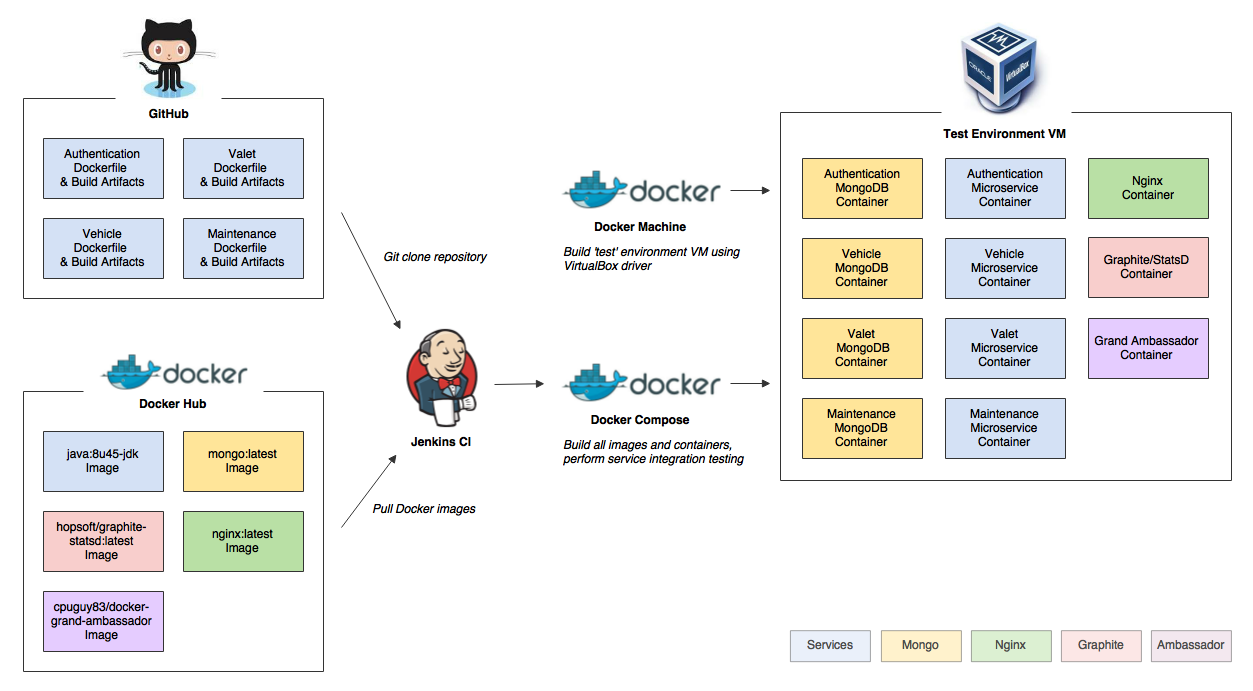
Introduction
In the last post, we learned how to use Jenkins CI, Maven, and Docker Compose to take a set of microservices all the way from source control on GitHub, to a fully tested and running set of integrated Docker containers. We built the microservices, Docker images, and Docker containers. We deployed the containers directly onto the Jenkins CI Server machine. Finally, we performed integration tests to ensure the services were functioning as expected, within the containers.
In a more mature continuous delivery model, we would have deployed the running containers to a fresh ‘production-like’ environment to be more accurately tested, not the Jenkins CI Server host machine. In this post, we will learn how to use the recently released Docker Machine to create a fresh test environment in which to build and host our project’s ten Docker containers. We will couple Docker Machine with Oracle’s VirtualBox, Jenkins CI, and Docker Compose to automatically build and test the services within their containers, within the virtual ‘test’ environment.
Update: All code for this post is available on GitHub, release version v2.1.0 on the ‘master’ branch (after running git clone …, run a ‘git checkout tags/v2.1.0’ command).
Docker Machine
If you recall in the last post, after compiling and packaging the microservices, Jenkins was used to deploy the build artifacts to the Virtual-Vehicles Docker GitHub project, as shown below.

We then used Jenkins, with the Docker CLI and the Docker Compose CLI, to automatically build and test the images and containers. This step will not change, however first we will use Docker Machine to automatically build a test environment, in which we will build the Docker images and containers.
I’ve copied and modified the second Jenkins job we used in the last post, as shown below. The new job is titled, ‘Virtual-Vehicles_Docker_Machine’. This will replace the previous job, ‘Virtual-Vehicles_Docker_Compose’.

The first step in the new Jenkins job is to clone the Virtual-Vehicles Docker GitHub repository.

Next, Jenkins run a bash script to automatically build the test VM with Docker Machine, build the Docker images and containers with Docker Compose within the new VM, and finally test the services.
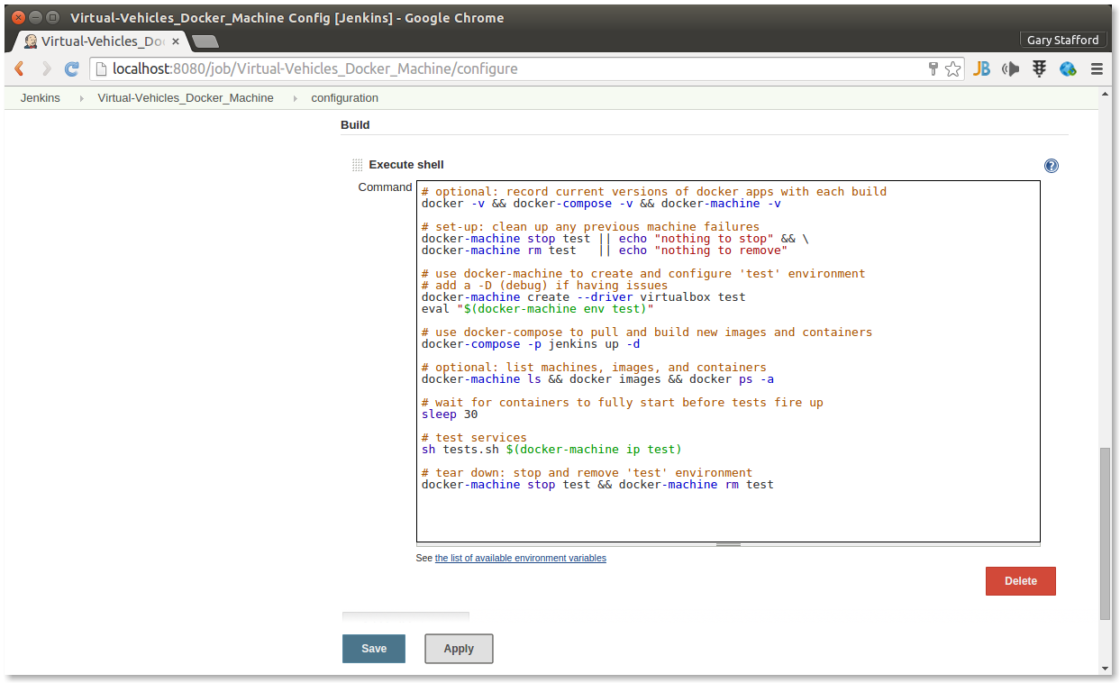
The bash script executed by Jenkins contains the following commands:
# optional: record current versions of docker apps with each build
docker -v && docker-compose -v && docker-machine -v

# set-up: clean up any previous machine failures
docker-machine stop test || echo "nothing to stop" && \
docker-machine rm test   || echo "nothing to remove"

# use docker-machine to create and configure 'test' environment
# add a -D (debug) if having issues
docker-machine create --driver virtualbox test
eval "$(docker-machine env test)"

# use docker-compose to pull and build new images and containers
docker-compose -p jenkins up -d

# optional: list machines, images, and containers
docker-machine ls && docker images && docker ps -a

# wait for containers to fully start before tests fire up
sleep 30

# test the services
sh tests.sh $(docker-machine ip test)

# tear down: stop and remove 'test' environment
docker-machine stop test && docker-machine rm test
As the above script shows, first Jenkins uses the Docker Machine CLI to build and activate the ‘test’ virtual machine, using the VirtualBox driver. As of docker-machine version 0.3.0, the VirtualBox driver requires at least VirtualBox 4.3.28 to be installed.
docker-machine create --driver virtualbox test
eval "$(docker-machine env test)"
Once this step is complete you will have the following VirtualBox VM created, running, and active.
NAME   ACTIVE   DRIVER       STATE     URL                         SWARM
test   *        virtualbox   Running   tcp://192.168.99.100:2376
Next, Jenkins uses the Docker Compose CLI to execute the project’s Docker Compose YAML file.
docker-compose -p jenkins up -d
The YAML file directs Docker Compose to pull and build the required Docker images, and to build and configure the Docker containers.
########################################################################
#
# title:       Docker Compose YAML file for Virtual-Vehicles Project
# author:      Gary A. Stafford (https://programmaticponderings.com)
# url:         https://github.com/garystafford/virtual-vehicles-docker
# description: Pulls (5) images, builds (5) images, and builds (11) containers,
#              for the Virtual-Vehicles Java microservices example REST API
# to run:      docker-compose -p <your_project_name_here> up -d
#
########################################################################

graphite:
  image: hopsoft/graphite-statsd:latest
  ports:
   - "8500:80"

mongoAuthentication:
  image: mongo:latest

mongoValet:
  image: mongo:latest

mongoMaintenance:
  image: mongo:latest

mongoVehicle:
  image: mongo:latest

authentication:
  build: authentication/
  links:
   - graphite
   - mongoAuthentication
   - "ambassador:nginx"
  expose:
   - "8587"

valet:
  build: valet/
  links:
   - graphite
   - mongoValet
   - "ambassador:nginx"
  expose:
   - "8585"

maintenance:
  build: maintenance/
  links:
   - graphite
   - mongoMaintenance
   - "ambassador:nginx"
  expose:
   - "8583"

vehicle:
  build: vehicle/
  links:
   - graphite
   - mongoVehicle
   - "ambassador:nginx"
  expose:
   - "8581"

nginx:
  build: nginx/
  ports:
   - "80:80"
  links:
   - "ambassador:vehicle"
   - "ambassador:valet"
   - "ambassador:authentication"
   - "ambassador:maintenance"

ambassador:
  image: cpuguy83/docker-grand-ambassador
  volumes:
   - "/var/run/docker.sock:/var/run/docker.sock"
  command: "-name jenkins_nginx_1 -name jenkins_authentication_1 -name jenkins_maintenance_1 -name jenkins_valet_1 -name jenkins_vehicle_1"
Running the docker-compose.yaml file, will pull these (5) Docker Hub images:
REPOSITORY                           TAG          IMAGE ID
==========                           ===          ========
java                                 8u45-jdk     1f80eb0f8128
nginx                                latest       319d2015d149
mongo                                latest       66b43e3cae49
hopsoft/graphite-statsd              latest       b03e373279e8
cpuguy83/docker-grand-ambassador     latest       c635b1699f78
And, build these (5) Docker images from Dockerfiles:
REPOSITORY                  TAG          IMAGE ID
==========                  ===          ========
jenkins_nginx               latest       0b53a9adb296
jenkins_vehicle             latest       d80f79e605f4
jenkins_valet               latest       cbe8bdf909b8
jenkins_maintenance         latest       15b8a94c00f4
jenkins_authentication      latest       ef0345369079
And, build these (11) Docker containers from corresponding image:
CONTAINER ID     IMAGE                                NAME
============     =====                                ====
17992acc6542     jenkins_nginx                        jenkins_nginx_1
bcbb2a4b1a7d     jenkins_vehicle                      jenkins_vehicle_1
4ac1ac69f230     mongo:latest                         jenkins_mongoVehicle_1
bcc8b9454103     jenkins_valet                        jenkins_valet_1
7c1794ca7b8c     jenkins_maintenance                  jenkins_maintenance_1
2d0e117fa5fb     jenkins_authentication               jenkins_authentication_1
d9146a1b1d89     hopsoft/graphite-statsd:latest       jenkins_graphite_1
56b34cee9cf3     cpuguy83/docker-grand-ambassador     jenkins_ambassador_1
a72199d51851     mongo:latest                         jenkins_mongoAuthentication_1
307cb2c01cc4     mongo:latest                         jenkins_mongoMaintenance_1
4e0807431479     mongo:latest                         jenkins_mongoValet_1
Since we are connected to the brand new Docker Machine ‘test’ VM, there are no locally cached Docker images. All images required to build the containers must be pulled from Docker Hub. The build time will be 3-4x as long as the last post’s build, which used the cached Docker images on the Jenkins CI machine.
Integration Testing
As in the last post, once the containers are built and configured, we run a series of expanded integration tests to confirm the containers and services are working. One difference, this time we will pass a parameter to the test bash script file:
sh tests.sh $(docker-machine ip test)
The parameter is the hostname used in the test’s RESTful service calls. The parameter, $(docker-machine ip test), is translated to the IP address of the ‘test’ VM. In our example, 192.168.99.100. If a parameter is not provided, the test script’s hostname variable will use the default value of localhost, ‘hostname=${1-'localhost'}‘.
Another change since the last post, the project now uses the open source version of Nginx, the free, open-source, high-performance HTTP server and reverse proxy, as a pseudo-API gateway. Instead calling each microservice directly, using their individual ports (i.e. port 8581 for the Vehicle microservice), all traffic is sent through Nginx on default http port 80, for example:
http://192.168.99.100/vehicles/utils/ping.json
http://192.168.99.100/jwts?apiKey=Z1nXG8JGKwvGlzQgPLwQdndW&secret=ODc4OGNiNjE5ZmI
http://192.168.99.100/vehicles/558f3042e4b0e562c03329ad
Internal traffic between the microservices and MongoDB, and between the microservices and Graphite is still direct, using Docker container linking. Traffic between the microservices and Nginx, in both directions, is handled by an ambassador container, a common pattern. Nginx acts as a reverse proxy for the microservices. Using Nginx brings us closer to a truer production-like experience for testing the services.
#!/bin/sh

########################################################################
#
# title:          Virtual-Vehicles Project Integration Tests
# author:         Gary A. Stafford (https://programmaticponderings.com)
# url:            https://github.com/garystafford/virtual-vehicles-docker
# description:    Performs integration tests on the Virtual-Vehicles
#                 microservices
# to run:         sh tests.sh
# docker-machine: sh tests.sh $(docker-machine ip test)
#
########################################################################

echo --- Integration Tests ---
echo

### VARIABLES ###
hostname=${1-'localhost'} # use input param or default to localhost
application="Test API Client $(date +%s)" # randomized
secret="$(date +%s | sha256sum | base64 | head -c 15)" # randomized
make="Test"
model="Foo"

echo hostname: ${hostname}
echo application: ${application}
echo secret: ${secret}
echo make: ${make}
echo model: ${model}
echo


### TESTS ###
echo "TEST: GET request should return 'true' in the response body"
url="http://${hostname}/vehicles/utils/ping.json"
echo ${url}
curl -X GET -H 'Accept: application/json; charset=UTF-8' \
--url "${url}" \
| grep true > /dev/null
[ "$?" -ne 0 ] && echo "RESULT: fail" && exit 1
echo "RESULT: pass"
echo


echo "TEST: POST request should return a new client in the response body with an 'id'"
url="http://${hostname}/clients"
echo ${url}
curl -X POST -H "Cache-Control: no-cache" -d "{
    \"application\": \"${application}\",
    \"secret\": \"${secret}\"
}" --url "${url}" \
| grep '"id":"[a-zA-Z0-9]\{24\}"' > /dev/null
[ "$?" -ne 0 ] && echo "RESULT: fail" && exit 1
echo "RESULT: pass"
echo


echo "SETUP: Get the new client's apiKey for next test"
url="http://${hostname}/clients"
echo ${url}
apiKey=$(curl -X POST -H "Cache-Control: no-cache" -d "{
    \"application\": \"${application}\",
    \"secret\": \"${secret}\"
}" --url "${url}" \
| grep -o '"apiKey":"[a-zA-Z0-9]\{24\}"' \
| grep -o '[a-zA-Z0-9]\{24\}' \
| sed -e 's/^"//'  -e 's/"$//')
echo apiKey: ${apiKey}
echo


echo "TEST: GET request should return a new jwt in the response body"
url="http://${hostname}/jwts?apiKey=${apiKey}&secret=${secret}"
echo ${url}
curl -X GET -H "Cache-Control: no-cache" \
--url "${url}" \
| grep '[a-zA-Z0-9_-]\{1,\}\.[a-zA-Z0-9_-]\{1,\}\.[a-zA-Z0-9_-]\{1,\}' > /dev/null
[ "$?" -ne 0 ] && echo "RESULT: fail" && exit 1
echo "RESULT: pass"
echo


echo "SETUP: Get a new jwt using the new client for the next test"
url="http://${hostname}/jwts?apiKey=${apiKey}&secret=${secret}"
echo ${url}
jwt=$(curl -X GET -H "Cache-Control: no-cache" \
--url "${url}" \
| grep '[a-zA-Z0-9_-]\{1,\}\.[a-zA-Z0-9_-]\{1,\}\.[a-zA-Z0-9_-]\{1,\}' \
| sed -e 's/^"//'  -e 's/"$//')
echo jwt: ${jwt}
echo


echo "TEST: POST request should return a new vehicle in the response body with an 'id'"
url="http://${hostname}/vehicles"
echo ${url}
curl -X POST -H "Cache-Control: no-cache" \
-H "Authorization: Bearer ${jwt}" \
-d "{
    \"year\": 2015,
    \"make\": \"${make}\",
    \"model\": \"${model}\",
    \"color\": \"White\",
    \"type\": \"Sedan\",
    \"mileage\": 250
}" --url "${url}" \
| grep '"id":"[a-zA-Z0-9]\{24\}"' > /dev/null
[ "$?" -ne 0 ] && echo "RESULT: fail" && exit 1
echo "RESULT: pass"
echo


echo "SETUP: Get id from new vehicle for the next test"
url="http://${hostname}/vehicles?filter=make::${make}|model::${model}&limit=1"
echo ${url}
id=$(curl -X GET -H "Cache-Control: no-cache" \
-H "Authorization: Bearer ${jwt}" \
--url "${url}" \
| grep '"id":"[a-zA-Z0-9]\{24\}"' \
| grep -o '[a-zA-Z0-9]\{24\}' \
| tail -1 \
| sed -e 's/^"//'  -e 's/"$//')
echo vehicle id: ${id}
echo


echo "TEST: GET request should return a vehicle in the response body with the requested 'id'"
url="http://${hostname}/vehicles/${id}"
echo ${url}
curl -X GET -H "Cache-Control: no-cache" \
-H "Authorization: Bearer ${jwt}" \
--url "${url}" \
| grep '"id":"[a-zA-Z0-9]\{24\}"' > /dev/null
[ "$?" -ne 0 ] && echo "RESULT: fail" && exit 1
echo "RESULT: pass"
echo


echo "TEST: POST request should return a new maintenance record in the response body with an 'id'"
url="http://${hostname}/maintenances"
echo ${url}
curl -X POST -H "Cache-Control: no-cache" \
-H "Authorization: Bearer ${jwt}" \
-d "{
    \"vehicleId\": \"${id}\",
    \"serviceDateTime\": \"2015-27-00T15:00:00.400Z\",
    \"mileage\": 1000,
    \"type\": \"Test Maintenance\",
    \"notes\": \"This is a test notes.\"
}" --url "${url}" \
| grep '"id":"[a-zA-Z0-9]\{24\}"' > /dev/null
[ "$?" -ne 0 ] && echo "RESULT: fail" && exit 1
echo "RESULT: pass"
echo


echo "TEST: POST request should return a new valet transaction in the response body with an 'id'"
url="http://${hostname}/valets"
echo ${url}
curl -X POST -H "Cache-Control: no-cache" \
-H "Authorization: Bearer ${jwt}" \
-d "{
    \"vehicleId\": \"${id}\",
    \"dateTimeIn\": \"2015-27-00T15:00:00.400Z\",
    \"parkingLot\": \"Test Parking Ramp\",
    \"parkingSpot\": 10,
    \"notes\": \"This is a test notes.\"
}" --url "${url}" \
| grep '"id":"[a-zA-Z0-9]\{24\}"' > /dev/null
[ "$?" -ne 0 ] && echo "RESULT: fail" && exit 1
echo "RESULT: pass"
echo
Tear Down
In true continuous integration fashion, once the integration tests have completed, we tear down the project by removing the VirtualBox ‘test’ VM. This also removed all images and containers.
docker-machine stop test && \
docker-machine rm test
Jenkins CI Console Output
Below is an abridged sample of what the Jenkins CI console output will look like from a successful ‘build’.
Started by user anonymous
Building in workspace /var/lib/jenkins/jobs/Virtual-Vehicles_Docker_Machine/workspace
> git rev-parse --is-inside-work-tree # timeout=10
Fetching changes from the remote Git repository
> git config remote.origin.url https://github.com/garystafford/virtual-vehicles-docker.git # timeout=10
Fetching upstream changes from https://github.com/garystafford/virtual-vehicles-docker.git
> git --version # timeout=10
using GIT_SSH to set credentials
using .gitcredentials to set credentials
> git config --local credential.helper store --file=/tmp/git7588068314920923143.credentials # timeout=10
> git -c core.askpass=true fetch --tags --progress https://github.com/garystafford/virtual-vehicles-docker.git +refs/heads/*:refs/remotes/origin/*
> git config --local --remove-section credential # timeout=10
> git rev-parse refs/remotes/origin/master^{commit} # timeout=10
> git rev-parse refs/remotes/origin/origin/master^{commit} # timeout=10
Checking out Revision f473249f0f70290b75cb320909af1f57cdaf2aa5 (refs/remotes/origin/master)
> git config core.sparsecheckout # timeout=10
> git checkout -f f473249f0f70290b75cb320909af1f57cdaf2aa5
> git rev-list f473249f0f70290b75cb320909af1f57cdaf2aa5 # timeout=10
[workspace] $ /bin/sh -xe /tmp/hudson8587699987350884629.sh

+ docker -v
Docker version 1.7.0, build 0baf609
+ docker-compose -v
docker-compose version: 1.3.1
CPython version: 2.7.9
OpenSSL version: OpenSSL 1.0.1e 11 Feb 2013
+ docker-machine -v
docker-machine version 0.3.0 (0a251fe)

+ docker-machine stop test
+ docker-machine rm test
Successfully removed test

+ docker-machine create --driver virtualbox test
Creating VirtualBox VM...
Creating SSH key...
Starting VirtualBox VM...
Starting VM...
To see how to connect Docker to this machine, run: docker-machine env test
+ docker-machine env test
+ eval export DOCKER_TLS_VERIFY="1"
export DOCKER_HOST="tcp://192.168.99.100:2376"
export DOCKER_CERT_PATH="/var/lib/jenkins/.docker/machine/machines/test"
export DOCKER_MACHINE_NAME="test"
# Run this command to configure your shell:
# eval "$(docker-machine env test)"
+ export DOCKER_TLS_VERIFY=1
+ export DOCKER_HOST=tcp://192.168.99.100:2376
+ export DOCKER_CERT_PATH=/var/lib/jenkins/.docker/machine/machines/test
+ export DOCKER_MACHINE_NAME=test
+ docker-compose -p jenkins up -d
Pulling mongoValet (mongo:latest)...
latest: Pulling from mongo

...Abridged output...

+ docker-machine ls
NAME   ACTIVE   DRIVER       STATE     URL                         SWARM
test   *        virtualbox   Running   tcp://192.168.99.100:2376
+ docker images
REPOSITORY                         TAG                 IMAGE ID            CREATED             VIRTUAL SIZE
jenkins_vehicle                    latest              fdd7f9d02ff7        2 seconds ago       837.1 MB
jenkins_valet                      latest              8a592e0fe69a        4 seconds ago       837.1 MB
jenkins_maintenance                latest              5a4a44e136e5        5 seconds ago       837.1 MB
jenkins_authentication             latest              e521e067a701        7 seconds ago       838.7 MB
jenkins_nginx                      latest              085d183df8b4        25 minutes ago      132.8 MB
java                               8u45-jdk            1f80eb0f8128        12 days ago         816.4 MB
nginx                              latest              319d2015d149        12 days ago         132.8 MB
mongo                              latest              66b43e3cae49        12 days ago         260.8 MB
hopsoft/graphite-statsd            latest              b03e373279e8        4 weeks ago         740 MB
cpuguy83/docker-grand-ambassador   latest              c635b1699f78        5 months ago        525.7 MB

+ docker ps -a
CONTAINER ID        IMAGE                              COMMAND                CREATED             STATUS              PORTS                                      NAMES
4ea39fa187bf        jenkins_vehicle                    "java -classpath .:c   2 seconds ago       Up 1 seconds        8581/tcp                                   jenkins_vehicle_1
b248a836546b        mongo:latest                       "/entrypoint.sh mong   3 seconds ago       Up 3 seconds        27017/tcp                                  jenkins_mongoVehicle_1
0c94e6409afc        jenkins_valet                      "java -classpath .:c   4 seconds ago       Up 3 seconds        8585/tcp                                   jenkins_valet_1
657f8432004b        jenkins_maintenance                "java -classpath .:c   5 seconds ago       Up 5 seconds        8583/tcp                                   jenkins_maintenance_1
8ff6de1208e3        jenkins_authentication             "java -classpath .:c   7 seconds ago       Up 6 seconds        8587/tcp                                   jenkins_authentication_1
c799d5f34a1c        hopsoft/graphite-statsd:latest     "/sbin/my_init"        12 minutes ago      Up 12 minutes       2003/tcp, 8125/udp, 0.0.0.0:8500->80/tcp   jenkins_graphite_1
040872881b25        jenkins_nginx                      "nginx -g 'daemon of   25 minutes ago      Up 25 minutes       0.0.0.0:80->80/tcp, 443/tcp                jenkins_nginx_1
c6a2dc726abc        mongo:latest                       "/entrypoint.sh mong   26 minutes ago      Up 26 minutes       27017/tcp                                  jenkins_mongoAuthentication_1
db22a44239f4        mongo:latest                       "/entrypoint.sh mong   26 minutes ago      Up 26 minutes       27017/tcp                                  jenkins_mongoMaintenance_1
d5fd655474ba        cpuguy83/docker-grand-ambassador   "/usr/bin/grand-amba   26 minutes ago      Up 26 minutes                                                  jenkins_ambassador_1
2b46bd6f8cfb        mongo:latest                       "/entrypoint.sh mong   31 minutes ago      Up 31 minutes       27017/tcp                                  jenkins_mongoValet_1

+ sleep 30

+ docker-machine ip test
+ sh tests.sh 192.168.99.100

--- Integration Tests ---

hostname: 192.168.99.100
application: Test API Client 1435585062
secret: NGM5OTI5ODAxMTZ
make: Test
model: Foo

TEST: GET request should return 'true' in the response body
http://192.168.99.100/vehicles/utils/ping.json
% Total    % Received % Xferd  Average Speed   Time    Time     Time  Current
Dload  Upload   Total   Spent    Left  Speed

0     0    0     0    0     0      0      0 --:--:-- --:--:-- --:--:--     0
100     4    0     4    0     0     26      0 --:--:-- --:--:-- --:--:--    25
100     4    0     4    0     0     26      0 --:--:-- --:--:-- --:--:--    25
RESULT: pass

TEST: POST request should return a new client in the response body with an 'id'
http://192.168.99.100/clients
% Total    % Received % Xferd  Average Speed   Time    Time     Time  Current
Dload  Upload   Total   Spent    Left  Speed

0     0    0     0    0     0      0      0 --:--:-- --:--:-- --:--:--     0
100   399    0   315  100    84    847    225 --:--:-- --:--:-- --:--:--   849
RESULT: pass

SETUP: Get the new client's apiKey for next test
http://192.168.99.100/clients
% Total    % Received % Xferd  Average Speed   Time    Time     Time  Current
Dload  Upload   Total   Spent    Left  Speed

0     0    0     0    0     0      0      0 --:--:-- --:--:-- --:--:--     0
100   399    0   315  100    84  20482   5461 --:--:-- --:--:-- --:--:-- 21000
apiKey: sv1CA9NdhmXh72NrGKBN3Abb

TEST: GET request should return a new jwt in the response body
http://192.168.99.100/jwts?apiKey=sv1CA9NdhmXh72NrGKBN3Abb&secret=NGM5OTI5ODAxMTZ
% Total    % Received % Xferd  Average Speed   Time    Time     Time  Current
Dload  Upload   Total   Spent    Left  Speed

0     0    0     0    0     0      0      0 --:--:-- --:--:-- --:--:--     0
100   222    0   222    0     0    686      0 --:--:-- --:--:-- --:--:--   687
RESULT: pass

SETUP: Get a new jwt using the new client for the next test
http://192.168.99.100/jwts?apiKey=sv1CA9NdhmXh72NrGKBN3Abb&secret=NGM5OTI5ODAxMTZ
% Total    % Received % Xferd  Average Speed   Time    Time     Time  Current
Dload  Upload   Total   Spent    Left  Speed

0     0    0     0    0     0      0      0 --:--:-- --:--:-- --:--:--     0
100   222    0   222    0     0  16843      0 --:--:-- --:--:-- --:--:-- 17076
jwt: eyJ0eXAiOiJKV1QiLCJhbGciOiJIUzI1NiJ9.eyJpc3MiOiJhcGkudmlydHVhbC12ZWhpY2xlcy5jb20iLCJhcGlLZXkiOiJzdjFDQTlOZGhtWGg3Mk5yR0tCTjNBYmIiLCJleHAiOjE0MzU2MjEwNjMsImFpdCI6MTQzNTU4NTA2M30.WVlhIhUcTz6bt3iMVr6MWCPIDd6P0aDZHl_iUd6AgrM

TEST: POST request should return a new vehicle in the response body with an 'id'
http://192.168.99.100/vehicles
% Total    % Received % Xferd  Average Speed   Time    Time     Time  Current
Dload  Upload   Total   Spent    Left  Speed

0     0    0     0    0     0      0      0 --:--:-- --:--:-- --:--:--     0
100   123    0     0  100   123      0    612 --:--:-- --:--:-- --:--:--   611
100   419    0   296  100   123    649    270 --:--:-- --:--:-- --:--:--   649
RESULT: pass

SETUP: Get id from new vehicle for the next test
http://192.168.99.100/vehicles?filter=make::Test|model::Foo&limit=1
% Total    % Received % Xferd  Average Speed   Time    Time     Time  Current
Dload  Upload   Total   Spent    Left  Speed

0     0    0     0    0     0      0      0 --:--:-- --:--:-- --:--:--     0
100   377    0   377    0     0   5564      0 --:--:-- --:--:-- --:--:--  5626
vehicle id: 55914a28e4b04658471dc03a

TEST: GET request should return a vehicle in the response body with the requested 'id'
http://192.168.99.100/vehicles/55914a28e4b04658471dc03a
% Total    % Received % Xferd  Average Speed   Time    Time     Time  Current
Dload  Upload   Total   Spent    Left  Speed

0     0    0     0    0     0      0      0 --:--:-- --:--:-- --:--:--     0
100   296    0   296    0     0   7051      0 --:--:-- --:--:-- --:--:--  7219
RESULT: pass

TEST: POST request should return a new maintenance record in the response body with an 'id'
http://192.168.99.100/maintenances
% Total    % Received % Xferd  Average Speed   Time    Time     Time  Current
Dload  Upload   Total   Spent    Left  Speed

0     0    0     0    0     0      0      0 --:--:-- --:--:-- --:--:--     0
100   565    0   376  100   189    506    254 --:--:-- --:--:-- --:--:--   506
100   565    0   376  100   189    506    254 --:--:-- --:--:-- --:--:--   506
RESULT: pass

TEST: POST request should return a new valet transaction in the response body with an 'id'
http://192.168.99.100/valets
% Total    % Received % Xferd  Average Speed   Time    Time     Time  Current
Dload  Upload   Total   Spent    Left  Speed

0     0    0     0    0     0      0      0 --:--:-- --:--:-- --:--:--     0
100   561    0   368  100   193    514    269 --:--:-- --:--:-- --:--:--   514
RESULT: pass

+ docker-machine stop test
+ docker-machine rm test
Successfully removed test

Finished: SUCCESS
Graphite and Statsd
If you’ve chose to build the Virtual-Vehicles Docker project outside of Jenkins CI, then in addition running the test script and using applications like Postman to test the Virtual-Vehicles RESTful API, you may also use Graphite and StatsD. RestExpress comes fully configured out of the box with Graphite integration, through the Metrics plugin. The Virtual-Vehicles RESTful API example is configured to use port 8500 to access the Graphite UI. The Virtual-Vehicles RESTful API example uses the hopsoft/graphite-statsd Docker image to build the Graphite/StatsD Docker container.

The Complete Process
The below diagram show the entire Virtual-Vehicles continuous integration and delivery process, start to finish, using Docker, Docker Hub, Docker Machine, Docker Compose, Jenkins CI, Maven, RestExpress, and VirtualBox.
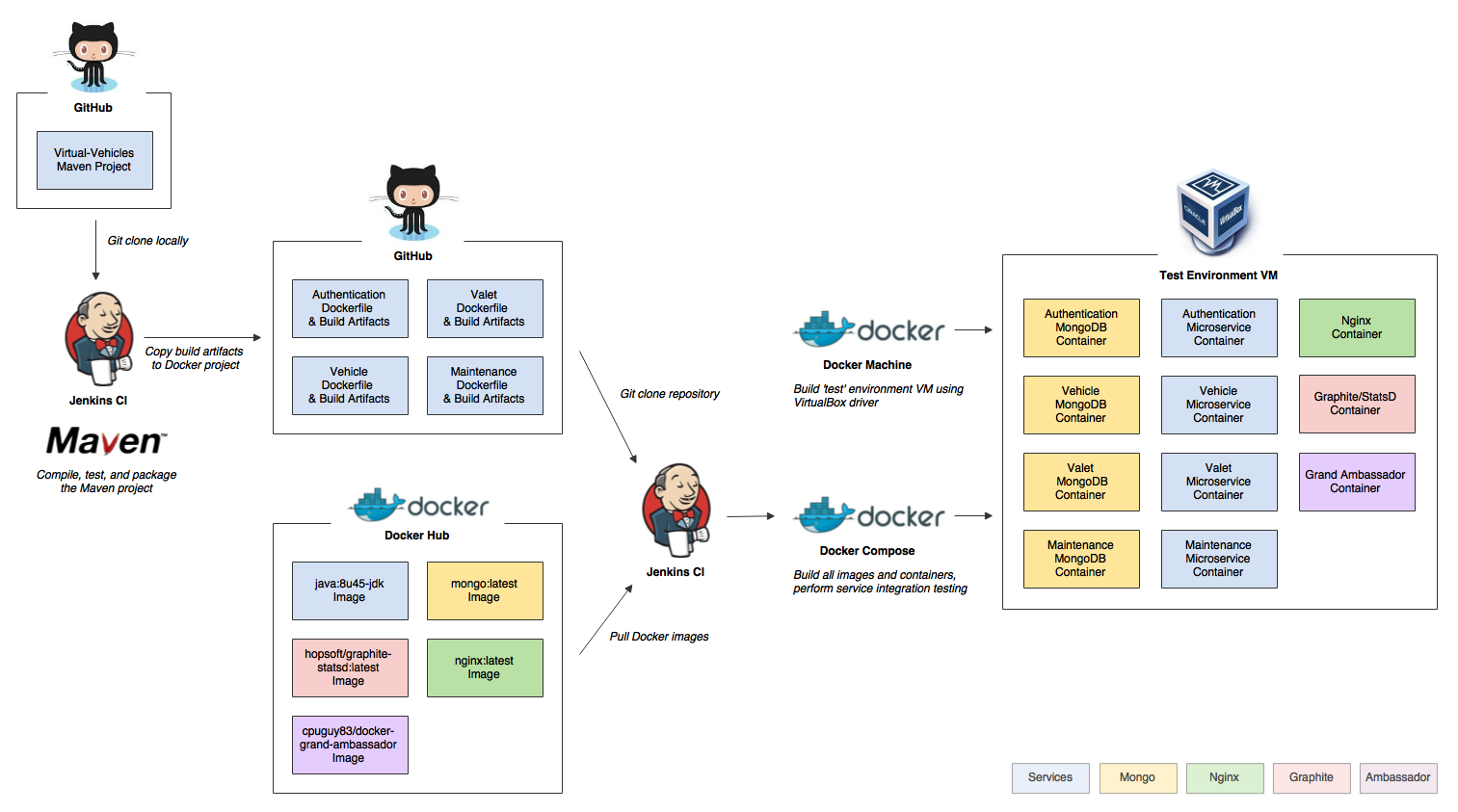
Continuous Integration and Delivery of Microservices using Jenkins CI, Maven, and Docker Compose
Posted by Gary A. Stafford in Bash Scripting, Build Automation, Continuous Delivery, DevOps, Enterprise Software Development on June 22, 2015
Continuously build, test, package and deploy a microservices-based, multi-container, Java EE application using Jenkins CI, Maven, Docker, and Docker Compose
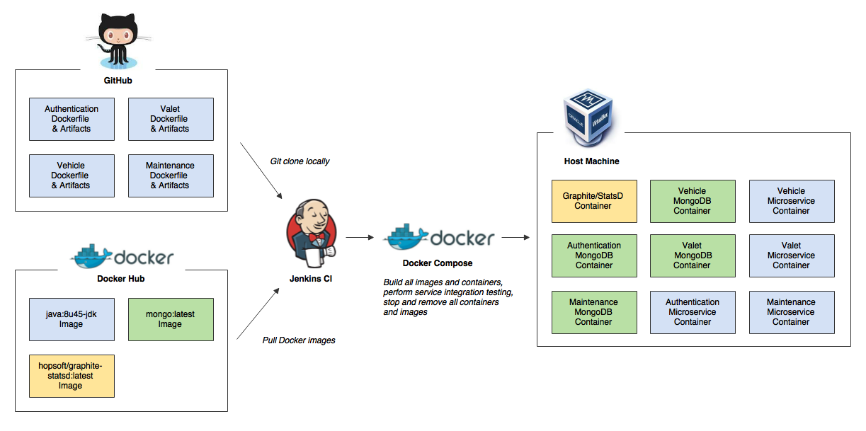
Previous Posts
In the previous 3-part series, Building a Microservices-based REST API with RestExpress, Java EE, and MongoDB, we developed a set of Java EE-based microservices, which formed the Virtual-Vehicles REST API. In Part One of this series, we introduced the concepts of a RESTful API and microservices, using the vehicle-themed Virtual-Vehicles REST API example. In Part Two, we gained a basic understanding of how RestExpress works to build microservices, and discovered how to get the microservices example up and running. Lastly, in Part Three, we explored how to use tools such as Postman, along with the API documentation, to test our microservices.
Introduction
In this post, we will demonstrate how to use Jenkins CI, Maven, and Docker Compose to take our set of microservices all the way from source control on GitHub, to a fully tested and running set of integrated and orchestrated Docker containers. We will build and test the microservices, Docker images, and Docker containers. We will deploy the containers and perform integration tests to ensure the services are functioning as expected, within the containers. The milestones in our process will be:
- Continuous Integration: Using Jenkins CI and Maven, automatically compile, test, and package the individual microservices
- Deployment: Using Jenkins, automatically deploy the build artifacts to the new Virtual-Vehicles Docker project
- Containerization: Using Jenkins and Docker Compose, automatically build the Docker images and containers from the build artifacts and a set of Dockerfiles
- Integration Testing: Using Jenkins, perform automated integration tests on the containerized services
- Tear Down: Using Jenkins, automatically stop and remove the containers and images
For brevity, we will deploy the containers directly to the Jenkins CI Server, where they were built. In an upcoming post, I will demonstrate how to use the recently released Docker Machine to host the containers within an isolated VM.
Note: All code for this post is available on GitHub, release version v1.0.0 on the ‘master’ branch (after running git clone …, run a ‘git checkout tags/v1.0.0’ command).
Build the Microservices
In order to host the Virtual-Vehicles microservices, we must first compile the source code and produce build artifacts. In the case of the Virtual-Vehicles example, the build artifacts are a JAR file and at least one environment-specific properties file. In Part Two of our previous series, we compiled and produced JAR files for our microservices from the command line using Maven.

To automatically build our Maven-based microservices project in this post, we will use Jenkins CI and the Jenkins Maven Project Plugin. The Virtual-Vehicles microservices are bundled together into what Maven considers a multi-module project, which is defined by a parent POM referring to one or more sub-modules. Using the concept of project inheritance, Jenkins will compile each of the four microservices from the project’s single parent POM file. Note the four modules at the end of the pom.xml below, corresponding to each microservice.
<?xml version="1.0" encoding="UTF-8"?>
<project xmlns="http://maven.apache.org/POM/4.0.0" xmlns:xsi="http://www.w3.org/2001/XMLSchema-instance" xsi:schemaLocation="http://maven.apache.org/POM/4.0.0 http://maven.apache.org/xsd/maven-4.0.0.xsd">
    <modelVersion>4.0.0</modelVersion>

    <name>Virtual-Vehicles API</name>
    <description>Virtual-Vehicles API
        https://maven.apache.org/guides/introduction/introduction-to-the-pom.html#Example_3
    </description>
    <url>https://github.com/garystafford/virtual-vehicle-demo</url>
    <groupId>com.example</groupId>
    <artifactId>Virtual-Vehicles-API</artifactId>
    <version>1</version>
    <packaging>pom</packaging>

    <modules>
        <module>Maintenance</module>
        <module>Valet</module>
        <module>Vehicle</module>
        <module>Authentication</module>
    </modules>
</project>
Below is the view of the four individual Maven modules, within the single Jenkins Maven job.

Each microservice module contains a Maven POM files. The POM files use the Apache Maven Compiler Plugin to compile code, and the Apache Maven Shade Plugin to create ‘uber-jars’ from the compiled code. The Shade plugin provides the capability to package the artifact in an uber-jar, including its dependencies. This will allow us to independently host the service in its own container, without external dependencies. Lastly, using the Apache Maven Resources Plugin, Maven will copy the environment properties files from the source directory to the ‘target’ directory, which contains the JAR file. To accomplish these Maven tasks, all Jenkins needs to do is a series of Maven life-cycle goals: ‘clean install package validate‘.
Once the code is compiled and packaged into uber-jars, Jenkins uses the Artifact Deployer Plugin to deploy the build artifacts from Jenkins’ workspace to a remote location. In our example, we will copy the artifacts to a second GitHub project, from which we will containerize our microservices.
Shown below are the two Jenkins jobs. The first one compiles, packages, and deploys the build artifacts. The second job containerizes the services, databases, and monitoring application.

Shown below are two screen grabs showing how we clone the Virtual-Vehicles GitHub repository and build the project using the main parent pom.xml file. Building the parent POM, in-turn builds all the microservice modules, using their POM files.


Deploy Build Artifacts
Once we have successfully compiled, tested (if we had unit tests with RestExpress), and packages the build artifacts as uber-jars, we deploy each set of build artifacts to a subfolder within the Virtual-Vehicles Docker GitHub project, using Jenkins’ Artifact Deployer Plugin. Shown below is the deployment configuration for just the Vehicles microservice. This deployment pattern is repeated for each service, within the Jenkins job configuration.

The Jenkins’ Artifact Deployer Plugin also provides the convenient ability to view and to redeploy the artifacts. Below, you see a list of the microservice artifacts deployed to the Docker project by Jenkins.
Build and Compose the Containers
The second Jenkins job clones the Virtual-Vehicles Docker GitHub repository.

The second Jenkins job executes commands from the shell prompt. The first commands use the Docker CLI to removes any existing images and containers, which might have been left over from previous job failures. The second commands use the Docker Compose CLI to execute the project’s Docker Compose YAML file. The YAML file directs Docker Compose to pull and build the required Docker images, and to build and configure the Docker containers.
# remove all images and containers from this build
docker ps -a --no-trunc  | grep 'jenkins' \
| awk '{print $1}' | xargs -r --no-run-if-empty docker stop && \
docker ps -a --no-trunc  | grep 'jenkins' \
| awk '{print $1}' | xargs -r --no-run-if-empty docker rm && \
docker images --no-trunc | grep 'jenkins' \
| awk '{print $3}' | xargs -r --no-run-if-empty docker rmi
# set DOCKER_HOST environment variable
export DOCKER_HOST=tcp://localhost:4243

# record installed version of Docker and Maven with each build
mvn --version && \
docker --version && \
docker-compose --version

# use docker-compose to build new images and containers
docker-compose -p jenkins up -d

# list virtual-vehicles related images
docker images | grep 'jenkins' | awk '{print $0}'

# list all containers
docker ps -a | grep 'jenkins\|mongo_\|graphite' | awk '{print $0}'
########################################################################
#
# title:       Docker Compose YAML file for Virtual-Vehicles Project
# author:      Gary A. Stafford (https://programmaticponderings.com)
# url:         https://github.com/garystafford/virtual-vehicles-docker
# description: Builds (4) images, pulls (2) images, and builds (9) containers,
#              for the Virtual-Vehicles Java microservices example REST API
# to run:      docker-compose -p virtualvehicles up -d
#
########################################################################

graphite:
  image: hopsoft/graphite-statsd:latest
  ports:
   - "8481:80"

mongoAuthentication:
  image: mongo:latest

mongoValet:
  image: mongo:latest

mongoMaintenance:
  image: mongo:latest

mongoVehicle:
  image: mongo:latest

authentication:
  build: authentication/
  ports:
   - "8587:8587"
  links:
   - graphite
   - mongoAuthentication

valet:
  build: valet/
  ports:
   - "8585:8585"
  links:
   - graphite
   - mongoValet
   - authentication

maintenance:
  build: maintenance/
  ports:
   - "8583:8583"
  links:
   - graphite
   - mongoMaintenance
   - authentication

vehicle:
  build: vehicle/
  ports:
   - "8581:8581"
  links:
   - graphite
   - mongoVehicle
   - authentication
Running the docker-compose.yaml file, produces the following images:
REPOSITORY                TAG        IMAGE ID
==========                ===        ========
jenkins_vehicle           latest     a6ea4dfe7cf5
jenkins_valet             latest     162d3102d43c
jenkins_maintenance       latest     0b6f530cc968
jenkins_authentication    latest     45b50487155e
And, these containers:
CONTAINER ID     IMAGE                              NAME
============     =====                              ====
2b4d5a918f1f     jenkins_vehicle                    jenkins_vehicle_1
492fbd88d267     mongo:latest                       jenkins_mongoVehicle_1
01f410bb1133     jenkins_valet                      jenkins_valet_1
6a63a664c335     jenkins_maintenance                jenkins_maintenance_1
00babf484cf7     jenkins_authentication             jenkins_authentication_1
548a31034c1e     hopsoft/graphite-statsd:latest     jenkins_graphite_1
cdc18bbb51b4     mongo:latest                       jenkins_mongoAuthentication_1
6be5c0558e92     mongo:latest                       jenkins_mongoMaintenance_1
8b71d50a4b4d     mongo:latest                       jenkins_mongoValet_1
Integration Testing
Once the containers have been successfully built and configured, we run a series of integration tests to confirm the services are up and running. We refer to these tests as integration tests because they test the interaction of multiple components. Integration tests were covered in the last post, Building a Microservices-based REST API with RestExpress, Java EE, and MongoDB: Part 3.
Note the short pause I have inserted before running the tests. Docker Compose does an excellent job of accounting for the required start-up order of the containers to avoid race conditions (see my previous post). However, depending on the speed of the host box, there is still a start-up period for the container’s processes to be up, running, and ready to receive traffic. Apache Log4j 2 and MongoDB startup, in particular, take extra time. I’ve seen the containers take as long as 1-2 minutes on a slow box to fully start. Without the pause, the tests fail with various errors, since the container’s processes are not all running.

sleep 15
sh tests.sh -v
The bash-based tests below just scratch the surface as a complete set of integration tests. However, they demonstrate an effective multi-stage testing pattern for handling the complex nature of RESTful service request requirements. The tests build upon each other. After setting up some variables, the tests register a new API client. Then, they use the new client’s API key to obtain a JWT. The tests then use the JWT to authenticate themselves, and create a new vehicle. Finally, they use the new vehicle’s id and the JWT to verify the existence for the new vehicle.
Although some may consider using bash to test somewhat primitive, the script demonstrates the effectiveness of bash’s curl, grep, sed, awk, along with regular expressions, to test our RESTful services.
#!/bin/sh

########################################################################
#
# title:       Virtual-Vehicles Project Integration Tests
# author:      Gary A. Stafford (https://programmaticponderings.com)
# url:         https://github.com/garystafford/virtual-vehicles-docker
# description: Performs integration tests on the Virtual-Vehicles
#              microservices
# to run:      sh tests.sh -v
#
########################################################################

echo --- Integration Tests ---

### VARIABLES ###
hostname="localhost"
application="Test API Client $(date +%s)" # randomized
secret="$(date +%s | sha256sum | base64 | head -c 15)" # randomized

echo hostname: ${hostname}
echo application: ${application}
echo secret: ${secret}


### TESTS ###
echo "TEST: GET request should return 'true' in the response body"
url="http://${hostname}:8581/vehicles/utils/ping.json"
echo ${url}
curl -X GET -H 'Accept: application/json; charset=UTF-8' \
--url "${url}" \
| grep true > /dev/null
[ "$?" -ne 0 ] && echo "RESULT: fail" && exit 1
echo "RESULT: pass"


echo "TEST: POST request should return a new client in the response body with an 'id'"
url="http://${hostname}:8587/clients"
echo ${url}
curl -X POST -H "Cache-Control: no-cache" -d "{
    \"application\": \"${application}\",
    \"secret\": \"${secret}\"
}" --url "${url}" \
| grep '"id":"[a-zA-Z0-9]\{24\}"' > /dev/null
[ "$?" -ne 0 ] && echo "RESULT: fail" && exit 1
echo "RESULT: pass"


echo "SETUP: Get the new client's apiKey for next test"
url="http://${hostname}:8587/clients"
echo ${url}
apiKey=$(curl -X POST -H "Cache-Control: no-cache" -d "{
    \"application\": \"${application}\",
    \"secret\": \"${secret}\"
}" --url "${url}" \
| grep -o '"apiKey":"[a-zA-Z0-9]\{24\}"' \
| grep -o '[a-zA-Z0-9]\{24\}' \
| sed -e 's/^"//'  -e 's/"$//')
echo apiKey: ${apiKey}
echo

echo "TEST: GET request should return a new jwt in the response body"
url="http://${hostname}:8587/jwts?apiKey=${apiKey}&secret=${secret}"
echo ${url}
curl -X GET -H "Cache-Control: no-cache" \
--url "${url}" \
| grep '[a-zA-Z0-9_-]\{1,\}\.[a-zA-Z0-9_-]\{1,\}\.[a-zA-Z0-9_-]\{1,\}' > /dev/null
[ "$?" -ne 0 ] && echo "RESULT: fail" && exit 1
echo "RESULT: pass"


echo "SETUP: Get a new jwt using the new client for the next test"
url="http://${hostname}:8587/jwts?apiKey=${apiKey}&secret=${secret}"
echo ${url}
jwt=$(curl -X GET -H "Cache-Control: no-cache" \
--url "${url}" \
| grep '[a-zA-Z0-9_-]\{1,\}\.[a-zA-Z0-9_-]\{1,\}\.[a-zA-Z0-9_-]\{1,\}' \
| sed -e 's/^"//'  -e 's/"$//')
echo jwt: ${jwt}


echo "TEST: POST request should return a new vehicle in the response body with an 'id'"
url="http://${hostname}:8581/vehicles"
echo ${url}
curl -X POST -H "Cache-Control: no-cache" \
-H "Authorization: Bearer ${jwt}" \
-d '{
    "year": 2015,
    "make": "Test",
    "model": "Foo",
    "color": "White",
    "type": "Sedan",
    "mileage": 250
}' --url "${url}" \
| grep '"id":"[a-zA-Z0-9]\{24\}"' > /dev/null
[ "$?" -ne 0 ] && echo "RESULT: fail" && exit 1
echo "RESULT: pass"


echo "SETUP: Get id from new vehicle for the next test"
url="http://${hostname}:8581/vehicles?filter=make::Test|model::Foo&limit=1"
echo ${url}
id=$(curl -X GET -H "Cache-Control: no-cache" \
-H "Authorization: Bearer ${jwt}" \
--url "${url}" \
| grep '"id":"[a-zA-Z0-9]\{24\}"' \
| grep -o '[a-zA-Z0-9]\{24\}' \
| tail -1 \
| sed -e 's/^"//'  -e 's/"$//')
echo vehicle id: ${id}


echo "TEST: GET request should return a vehicle in the response body with the requested 'id'"
url="http://${hostname}:8581/vehicles/${id}"
echo ${url}
curl -X GET -H "Cache-Control: no-cache" \
-H "Authorization: Bearer ${jwt}" \
--url "${url}" \
| grep '"id":"[a-zA-Z0-9]\{24\}"' > /dev/null
[ "$?" -ne 0 ] && echo "RESULT: fail" && exit 1
echo "RESULT: pass"
Since our tests are just a bash script, they can also be ran separately from the command line, as in the screen grab below. The output, except for the colored text, is identical to what appears in the Jenkins console output.
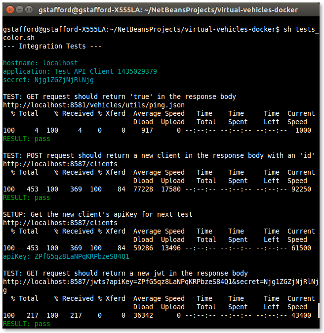
Tear Down
Once the integration tests have completed, we ‘tear down’ the project by removing the Virtual-Vehicle images and containers. We simply repeat the first commands we ran at the start of the Jenkins build phase. You could choose to remove the tear down step, and use this job as a way to simply build and start your multi-container application.
# remove all images and containers from this build
docker ps -a --no-trunc  | grep 'jenkins' \
| awk '{print $1}' | xargs -r --no-run-if-empty docker stop && \
docker ps -a --no-trunc  | grep 'jenkins' \
| awk '{print $1}' | xargs -r --no-run-if-empty docker rm && \
docker images --no-trunc | grep 'jenkins' \
| awk '{print $3}' | xargs -r --no-run-if-empty docker rmi
The Complete Process
The below diagram show the entire process, start to finish.

Gary Stafford
AWS Area Principal Solutions Architect | 10x AWS Certified Pro | DevOps | Data/ML | Serverless | Polyglot Developer | Former ThoughtWorks and Accenture
