Posts Tagged docker

Continuous Integration and Deployment of Docker Images using GitHub Actions

Posted by Gary A. Stafford in Build Automation, Cloud, Continuous Delivery, DevOps, Go, Kubernetes, Software Development on June 16, 2021

According to GitHub, GitHub Actions allows you to automate, customize, and execute your software development workflows right in your repository. You can discover, create, and share actions to perform any job you would like, including continuous integration (CI) and continuous deployment (CD), and combine actions in a completely customized workflow.

This brief post will examine a simple use case for GitHub Actions — automatically building and pushing a new Docker image to Docker Hub. A GitHub Actions workflow will be triggered every time a new Git tag is pushed to the GitHub project repository.

GitHub Actions Workflow running, based on the push of a new git tag

GitHub Project Repository

For the demonstration, we will be using the public NLP Client microservice GitHub project repository. The NLP Client, written in Go, is part of five microservices that comprise the Natural Language Processing (NLP) API. I developed this API to demonstrate architectural principles and DevOps practices. The API’s microservices are designed to be run as a distributed system using container orchestration platforms such as Docker Swarm, Red Hat OpenShift, Amazon ECS, and Kubernetes.

Encrypted Secrets

To push new images to Docker Hub, the workflow must be logged in to your Docker Hub account. GitHub recommends storing your Docker Hub username and password as encrypted secrets, so they are not exposed in your workflow file. Encrypted secrets allow you to store sensitive information as encrypted environment variables in your organization, repository, or repository environment. The secrets that you create will be available to use in GitHub Actions workflows. To allow the workflow to log in to Docker Hub, I created two secrets, DOCKERHUB_USERNAME and DOCKERHUB_PASSWORD using my organization’s credentials, which I then reference in the workflow.

Actions Secrets shown in the GitHub project’s Secrets tab

GitHub Actions Workflow

According to GitHub, a workflow is a configurable automated process made up of one or more jobs. You must create a YAML file to define your workflow configuration. GitHub contains many searchable code examples you can use to bootstrap your workflow development. For this demonstration, I started with the example shown in the GitHub Actions Guide, Publishing Docker images, and modified it to meet my needs. Workflow files are checked into the project’s repository within the .github/workflows directory.https://itnext.io/media/0e27d26012167bab83def6ef3595a74f

Workflow Development

Visual Studio Code (VS Code) is an excellent, full-featured, and free IDE for software development and writing Infrastructure as Code (IaC). VS Code has a large ecosystem of extensions, including extensions for GitHub Actions. Currently, I am using the GitHub Actions extension, cschleiden.vscode-github-actions, by Christopher Schleiden.

The extension features auto-complete, as shown below in the GitHub Actions workflow YAML file.

Auto-complete example using the GitHub Actions extension

Git Tags

The demonstration’s workflow is designed to be triggered when a new Git tag is pushed to the NLP Client project repository. Using the workflow, you can perform normal pushes (git push) to the repository without triggering the workflow. For example, you would not typically want to trigger a new image build and push when updating the project’s README file. Thus, we use the new Git tag as the workflow trigger.

Git tags as shown in the GitHub project repository

For consistency, I also designed the workflow to be triggered only when the format of the Git tag follows the common Semantic Versioning (SemVer) convention of version number MAJOR.MINOR.PATCH (v*.*.*).

on:
  push:
    tags:
      - 'v*.*.*'

Also, following common Docker conventions in the workflow, the Git tag (e.g., v1.2.3) is truncated to remove the letter ‘v’ and used as the tag for the Docker image (e.g., 1.2.3). In the workflow, theGITHUB_REF:11 portion of the command truncates the Git tag reference of refs/tags/v1.2.3 to just 1.2.3.

run: echo "RELEASE_VERSION=${GITHUB_REF:11}" >> $GITHUB_ENV

Workflow Run

Pushing the Git tag triggers the workflow to run automatically, as seen in the Actions tab.

Detailed logs show you how each step in the workflow was processed.

The example below shows that the workflow has successfully built and pushed a new Docker image to Docker Hub for the NLP Client microservice.

Failure Notifications

You can choose to receive a notification when a workflow fails. GitHub Actions notifications are a configurable option found in the GitHub account owner’s Settings tab.

Example email notification of workflow run failure

Status Badge

You can display a status badge in your repository to indicate the status of your workflows. The badge can be added as Markdown to your README file.

Docker Hub

As a result of the successful completion of the workflow, we now have a new image tagged as 1.2.3 in the NLP Client Docker Hub repository: garystafford/nlp-client.

Conclusion

In this brief post, we saw a simple example of how GitHub Actions allows you to automate, customize, and execute your software development workflows right in your GitHub repository. We can easily extend this post’s GitHub Actions example to include updating the service’s Kubernetes Deployment resource file to the latest image tag in Docker Hub. Further, we can trigger a GitOps workflow with tools such as Weaveworks’ Flux or Argo CD to deploy the revised workload to a Kubernetes cluster.

This blog represents my own viewpoints and not of my employer, Amazon Web Services (AWS). All product names, logos, and brands are the property of their respective owners.

DevOps, docker, GitHub, GitHub Actions

Getting Started with Data Analytics using Jupyter Notebooks, PySpark, and Docker

Posted by Gary A. Stafford in Bash Scripting, Big Data, Build Automation, DevOps, Python, Software Development on December 6, 2019

Audio Introduction

There is little question, big data analytics, data science, artificial intelligence (AI), and machine learning (ML), a subcategory of AI, have all experienced a tremendous surge in popularity over the last few years. Behind the marketing hype, these technologies are having a significant influence on many aspects of our modern lives. Due to their popularity and potential benefits, commercial enterprises, academic institutions, and the public sector are rushing to develop hardware and software solutions to lower the barriers to entry and increase the velocity of ML and Data Scientists and Engineers.

(courtesy Google Trends and Plotly)

Many open-source software projects are also lowering the barriers to entry into these technologies. An excellent example of one such open-source project working on this challenge is Project Jupyter. Similar to Apache Zeppelin and the newly open-sourced Netflix’s Polynote, Jupyter Notebooks enables data-driven, interactive, and collaborative data analytics.

This post will demonstrate the creation of a containerized data analytics environment using Jupyter Docker Stacks. The particular environment will be suited for learning and developing applications for Apache Spark using the Python, Scala, and R programming languages. We will focus on Python and Spark, using PySpark.

Featured Technologies

The following technologies are featured prominently in this post.

Jupyter Notebooks

According to Project Jupyter, the Jupyter Notebook, formerly known as the IPython Notebook, is an open-source web application that allows users to create and share documents that contain live code, equations, visualizations, and narrative text. Uses include data cleansing and transformation, numerical simulation, statistical modeling, data visualization, machine learning, and much more. The word, Jupyter, is a loose acronym for Julia, Python, and R, but today, Jupyter supports many programming languages.

Interest in Jupyter Notebooks has grown dramatically over the last 3–5 years, fueled in part by the major Cloud providers, AWS, Google Cloud, and Azure. Amazon Sagemaker, Amazon EMR (Elastic MapReduce), Google Cloud Dataproc, Google Colab (Collaboratory), and Microsoft Azure Notebooks all have direct integrations with Jupyter notebooks for big data analytics and machine learning.

(courtesy Google Trends and Plotly)

Jupyter Docker Stacks

To enable quick and easy access to Jupyter Notebooks, Project Jupyter has created Jupyter Docker Stacks. The stacks are ready-to-run Docker images containing Jupyter applications, along with accompanying technologies. Currently, the Jupyter Docker Stacks focus on a variety of specializations, including the r-notebook, scipy-notebook, tensorflow-notebook, datascience-notebook, pyspark-notebook, and the subject of this post, the all-spark-notebook. The stacks include a wide variety of well-known packages to extend their functionality, such as scikit-learn, pandas, Matplotlib, Bokeh, NumPy, and Facets.

Apache Spark

According to Apache, Spark is a unified analytics engine for large-scale data processing. Starting as a research project at the UC Berkeley AMPLab in 2009, Spark was open-sourced in early 2010 and moved to the Apache Software Foundation in 2013. Reviewing the postings on any major career site will confirm that Spark is widely used by well-known modern enterprises, such as Netflix, Adobe, Capital One, Lockheed Martin, JetBlue Airways, Visa, and Databricks. At the time of this post, LinkedIn, alone, had approximately 3,500 listings for jobs that reference the use of Apache Spark, just in the United States.

With speeds up to 100 times faster than Hadoop, Apache Spark achieves high performance for static, batch, and streaming data, using a state-of-the-art DAG (Directed Acyclic Graph) scheduler, a query optimizer, and a physical execution engine. Spark’s polyglot programming model allows users to write applications quickly in Scala, Java, Python, R, and SQL. Spark includes libraries for Spark SQL (DataFrames and Datasets), MLlib (Machine Learning), GraphX (Graph Processing), and DStreams (Spark Streaming). You can run Spark using its standalone cluster mode, Apache Hadoop YARN, Mesos, or Kubernetes.

PySpark

The Spark Python API, PySpark, exposes the Spark programming model to Python. PySpark is built on top of Spark’s Java API and uses Py4J. According to Apache, Py4J, a bridge between Python and Java, enables Python programs running in a Python interpreter to dynamically access Java objects in a Java Virtual Machine (JVM). Data is processed in Python and cached and shuffled in the JVM.

Docker

According to Docker, their technology gives developers and IT the freedom to build, manage, and secure business-critical applications without the fear of technology or infrastructure lock-in. For this post, I am using the current stable version of Docker Desktop Community version for macOS, as of March 2020.

Screen Shot 2020-03-07 at 9.16.03 PM

Docker Swarm

Current versions of Docker include both a Kubernetes and Swarm orchestrator for deploying and managing containers. We will choose Swarm for this demonstration. According to Docker, the cluster management and orchestration features embedded in the Docker Engine are built using swarmkit. Swarmkit is a separate project that implements Docker’s orchestration layer and is used directly within Docker.

PostgreSQL

PostgreSQL is a powerful, open-source, object-relational database system. According to their website, PostgreSQL comes with many features aimed to help developers build applications, administrators to protect data integrity and build fault-tolerant environments, and help manage data no matter how big or small the dataset.

Demonstration

In this demonstration, we will explore the capabilities of the Spark Jupyter Docker Stack to provide an effective data analytics development environment. We will explore a few everyday uses, including executing Python scripts, submitting PySpark jobs, and working with Jupyter Notebooks, and reading and writing data to and from different file formats and a database. We will be using the latest jupyter/all-spark-notebook Docker Image. This image includes Python, R, and Scala support for Apache Spark, using Apache Toree.

Architecture

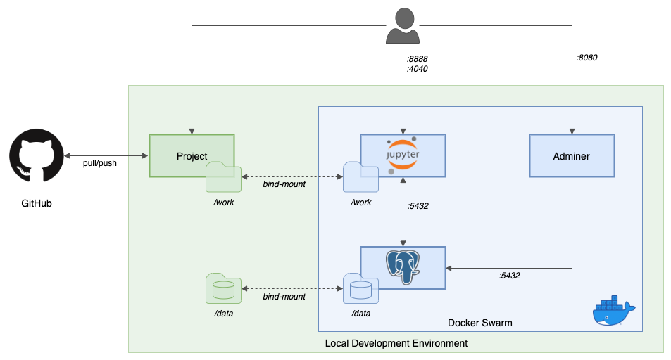
As shown below, we will deploy a Docker stack to a single-node Docker swarm. The stack consists of a Jupyter All-Spark-Notebook, PostgreSQL (Alpine Linux version 12), and Adminer container. The Docker stack will have two local directories bind-mounted into the containers. Files from our GitHub project will be shared with the Jupyter application container through a bind-mounted directory. Our PostgreSQL data will also be persisted through a bind-mounted directory. This allows us to persist data external to the ephemeral containers. If the containers are restarted or recreated, the data is preserved locally.

Source Code

All source code for this post can be found on GitHub. Use the following command to clone the project. Note this post uses the v2 branch.

git clone \
  --branch v2 --single-branch --depth 1 --no-tags \
  https://github.com/garystafford/pyspark-setup-demo.git

Source code samples are displayed as GitHub Gists, which may not display correctly on some mobile and social media browsers.

Deploy Docker Stack

To start, create the $HOME/data/postgres directory to store PostgreSQL data files.

mkdir -p ~/data/postgres

This directory will be bind-mounted into the PostgreSQL container on line 41 of the stack.yml file, $HOME/data/postgres:/var/lib/postgresql/data. The HOME environment variable assumes you are working on Linux or macOS and is equivalent to HOMEPATH on Windows.

The Jupyter container’s working directory is set on line 15 of the stack.yml file, working_dir: /home/$USER/work. The local bind-mounted working directory is $PWD/work. This path is bind-mounted to the working directory in the Jupyter container, on line 29 of the Docker stack file, $PWD/work:/home/$USER/work. The PWD environment variable assumes you are working on Linux or macOS (CD on Windows).

By default, the user within the Jupyter container is jovyan. We will override that user with our own local host’s user account, as shown on line 21 of the Docker stack file, NB_USER: $USER. We will use the host’s USER environment variable value (equivalent to USERNAME on Windows). There are additional options for configuring the Jupyter container. Several of those options are used on lines 17–22 of the Docker stack file (gist).

	# docker stack deploy -c stack.yml jupyter
	# optional pgadmin container
	version: "3.7"
	networks:
	demo-net:
	services:
	spark:
	image: jupyter/all-spark-notebook:latest
	ports:
	– "8888:8888/tcp"
	– "4040:4040/tcp"
	networks:
	– demo-net
	working_dir: /home/$USER/work
	environment:
	CHOWN_HOME: "yes"
	GRANT_SUDO: "yes"
	NB_UID: 1000
	NB_GID: 100
	NB_USER: $USER
	NB_GROUP: staff
	user: root
	deploy:
	replicas: 1
	restart_policy:
	condition: on-failure
	volumes:
	– $PWD/work:/home/$USER/work
	postgres:
	image: postgres:12-alpine
	environment:
	POSTGRES_USERNAME: postgres
	POSTGRES_PASSWORD: postgres1234
	POSTGRES_DB: bakery
	ports:
	– "5432:5432/tcp"
	networks:
	– demo-net
	volumes:
	– $HOME/data/postgres:/var/lib/postgresql/data
	deploy:
	restart_policy:
	condition: on-failure
	adminer:
	image: adminer:latest
	ports:
	– "8080:8080/tcp"
	networks:
	– demo-net
	deploy:
	restart_policy:
	condition: on-failure
	# pgadmin:
	# image: dpage/pgadmin4:latest
	# environment:
	# PGADMIN_DEFAULT_EMAIL: user@domain.com
	# PGADMIN_DEFAULT_PASSWORD: 5up3rS3cr3t!
	# ports:
	# – "8180:80/tcp"
	# networks:
	# – demo-net
	# deploy:
	# restart_policy:
	# condition: on-failure

view raw

stack.yml

hosted with ❤ by GitHub

The jupyter/all-spark-notebook Docker image is large, approximately 5 GB. Depending on your Internet connection, if this is the first time you have pulled this image, the stack may take several minutes to enter a running state. Although not required, I usually pull new Docker images in advance.

docker pull jupyter/all-spark-notebook:latest
docker pull postgres:12-alpine
docker pull adminer:latest

Assuming you have a recent version of Docker installed on your local development machine and running in swarm mode, standing up the stack is as easy as running the following docker command from the root directory of the project.

docker stack deploy -c stack.yml jupyter

The Docker stack consists of a new overlay network, jupyter_demo-net, and three containers. To confirm the stack deployed successfully, run the following docker command.

docker stack ps jupyter --no-trunc

To access the Jupyter Notebook application, you need to obtain the Jupyter URL and access token. The Jupyter URL and the access token are output to the Jupyter container log, which can be accessed with the following command.

docker logs $(docker ps | grep jupyter_spark | awk '{print $NF}')

You should observe log output similar to the following. Retrieve the complete URL, for example, http://127.0.0.1:8888/?token=f78cbe..., to access the Jupyter web-based user interface.

From the Jupyter dashboard landing page, you should see all the files in the project’s work/ directory. Note the types of files you can create from the dashboard, including Python 3, R, and Scala (using Apache Toree or spylon-kernal) notebooks, and text. You can also open a Jupyter terminal or create a new Folder from the drop-down menu. At the time of this post (March 2020), the latest jupyter/all-spark-notebook Docker Image runs Spark 2.4.5, Scala 2.11.12, Python 3.7.6, and OpenJDK 64-Bit Server VM, Java 1.8.0 Update 242.

Bootstrap Environment

Included in the project is a bootstrap script, bootstrap_jupyter.sh. The script will install the required Python packages using pip, the Python package installer, and a requirement.txt file. The bootstrap script also installs the latest PostgreSQL driver JAR, configures Apache Log4j to reduce log verbosity when submitting Spark jobs, and installs htop. Although these tasks could also be done from a Jupyter terminal or from within a Jupyter notebook, using a bootstrap script ensures you will have a consistent work environment every time you spin up the Jupyter Docker stack. Add or remove items from the bootstrap script as necessary.

	#!/bin/bash

	set -ex

	# update/upgrade and install htop
	sudo apt-get update -y && sudo apt-get upgrade -y
	sudo apt-get install htop

	# install required python packages
	python3 -m pip install –user –upgrade pip
	python3 -m pip install -r requirements.txt –upgrade

	# download latest postgres driver jar
	POSTGRES_JAR="postgresql-42.2.17.jar"
	if [ -f "$POSTGRES_JAR" ]; then
	echo "$POSTGRES_JAR exist"
	else
	wget -nv "https://jdbc.postgresql.org/download/${POSTGRES_JAR}"
	fi

	# spark-submit logging level from INFO to WARN
	sudo cp log4j.properties /usr/local/spark/conf/log4j.properties

view raw

bootstrap_jupyter.sh

hosted with ❤ by GitHub

That’s it, our new Jupyter environment is ready to start exploring.

Running Python Scripts

One of the simplest tasks we could perform in our new Jupyter environment is running Python scripts. Instead of worrying about installing and maintaining the correct versions of Python and multiple Python packages on your own development machine, we can run Python scripts from within the Jupyter container. At the time of this post update, the latest jupyter/all-spark-notebook Docker image runs Python 3.7.3 and Conda 4.7.12. Let’s start with a simple Python script, 01_simple_script.py.

	#!/usr/bin/python3

	import random

	technologies = [
	'PySpark', 'Python', 'Spark', 'Scala', 'Java', 'Project Jupyter', 'R'
	]

	print("Technologies: %s\n" % technologies)

	technologies.sort()
	print("Sorted: %s\n" % technologies)

	print("I'm interested in learning about %s." % random.choice(technologies))

view raw

01_simple_script.py

hosted with ❤ by GitHub

From a Jupyter terminal window, use the following command to run the script.

python3 01_simple_script.py

You should observe the following output.

Kaggle Datasets

To explore more features of the Jupyter and PySpark, we will use a publicly available dataset from Kaggle. Kaggle is an excellent open-source resource for datasets used for big-data and ML projects. Their tagline is ‘Kaggle is the place to do data science projects’. For this demonstration, we will use the Transactions from a bakery dataset from Kaggle. The dataset is available as a single CSV-format file. A copy is also included in the project.

The ‘Transactions from a bakery’ dataset contains 21,294 rows with 4 columns of data. Although certainly not big data, the dataset is large enough to test out the Spark Jupyter Docker Stack functionality. The data consists of 9,531 customer transactions for 21,294 bakery items between 2016-10-30 and 2017-04-09 (gist).

Date	Time	Transaction	Item
2016-10-30	09:58:11	1	Bread
2016-10-30	10:05:34	2	Scandinavian
2016-10-30	10:05:34	2	Scandinavian
2016-10-30	10:07:57	3	Hot chocolate
2016-10-30	10:07:57	3	Jam
2016-10-30	10:07:57	3	Cookies
2016-10-30	10:08:41	4	Muffin
2016-10-30	10:13:03	5	Coffee
2016-10-30	10:13:03	5	Pastry
2016-10-30	10:13:03	5	Bread

view raw

bakery_data.csv

hosted with ❤ by GitHub

Submitting Spark Jobs

We are not limited to Jupyter notebooks to interact with Spark. We can also submit scripts directly to Spark from the Jupyter terminal. This is typically how Spark is used in a Production for performing analysis on large datasets, often on a regular schedule, using tools such as Apache Airflow. With Spark, you are load data from one or more data sources. After performing operations and transformations on the data, the data is persisted to a datastore, such as a file or a database, or conveyed to another system for further processing.

The project includes a simple Python PySpark ETL script, 02_pyspark_job.py. The ETL script loads the original Kaggle Bakery dataset from the CSV file into memory, into a Spark DataFrame. The script then performs a simple Spark SQL query, calculating the total quantity of each type of bakery item sold, sorted in descending order. Finally, the script writes the results of the query to a new CSV file, output/items-sold.csv.

	#!/usr/bin/python3

	from pyspark.sql import SparkSession

	spark = SparkSession \
	.builder \
	.appName('spark-demo') \
	.getOrCreate()

	df_bakery = spark.read \
	.format('csv') \
	.option('header', 'true') \
	.option('delimiter', ',') \
	.option('inferSchema', 'true') \
	.load('BreadBasket_DMS.csv')

	df_sorted = df_bakery.cube('item').count() \
	.filter('item NOT LIKE \'NONE\'') \
	.filter('item NOT LIKE \'Adjustment\'') \
	.orderBy(['count', 'item'], ascending=[False, True])

	df_sorted.show(10, False)

	df_sorted.coalesce(1) \
	.write.format('csv') \
	.option('header', 'true') \
	.save('output/items-sold.csv', mode='overwrite')

view raw

02_bakery_dataframes.py

hosted with ❤ by GitHub

Run the script directly from a Jupyter terminal using the following command.

python3 02_pyspark_job.py

An example of the output of the Spark job is shown below.

Typically, you would submit the Spark job using the spark-submit command. Use a Jupyter terminal to run the following command.

$SPARK_HOME/bin/spark-submit 02_pyspark_job.py

Below, we see the output from the spark-submit command. Printing the results in the output is merely for the purposes of the demo. Typically, Spark jobs are submitted non-interactively, and the results are persisted directly to a datastore or conveyed to another system.

Using the following commands, we can view the resulting CVS file, created by the spark job.

ls -alh output/items-sold.csv/
head -5 output/items-sold.csv/*.csv

An example of the files created by the spark job is shown below. We should have discovered that coffee is the most commonly sold bakery item with 5,471 sales, followed by bread with 3,325 sales.

Interacting with Databases

To demonstrate the flexibility of Jupyter to work with databases, PostgreSQL is part of the Docker Stack. We can read and write data from the Jupyter container to the PostgreSQL instance, running in a separate container. To begin, we will run a SQL script, written in Python, to create our database schema and some test data in a new database table. To do so, we will use the psycopg2, the PostgreSQL database adapter package for the Python, we previously installed into our Jupyter container using the bootstrap script. The below Python script, 03_load_sql.py, will execute a set of SQL statements contained in a SQL file, bakery.sql, against the PostgreSQL container instance.

	#!/usr/bin/python3

	import psycopg2

	# connect to database
	connect_str = 'host=postgres port=5432 dbname=bakery user=postgres password=postgres1234'
	conn = psycopg2.connect(connect_str)
	conn.autocommit = True
	cursor = conn.cursor()

	# execute sql script
	sql_file = open('bakery.sql', 'r')
	sqlFile = sql_file.read()
	sql_file.close()
	sqlCommands = sqlFile.split(';')
	for command in sqlCommands:
	print(command)
	if command.strip() != '':
	cursor.execute(command)

	# import data from csv file
	with open('BreadBasket_DMS.csv', 'r') as f:
	next(f) # Skip the header row.
	cursor.copy_from(
	f,
	'transactions',
	sep=',',
	columns=('date', 'time', 'transaction', 'item')
	)
	conn.commit()

	# confirm by selecting record
	command = 'SELECT COUNT(*) FROM public.transactions;'
	cursor.execute(command)
	recs = cursor.fetchall()
	print('Row count: %d' % recs[0])

view raw

03_load_sql.py

hosted with ❤ by GitHub

The SQL file, bakery.sql.

	DROP TABLE IF EXISTS "transactions";
	DROP SEQUENCE IF EXISTS transactions_id_seq;
	CREATE SEQUENCE transactions_id_seq INCREMENT 1 MINVALUE 1 MAXVALUE 2147483647 START 1 CACHE 1;

	CREATE TABLE "public"."transactions"
	(
	"id" integer DEFAULT nextval('transactions_id_seq') NOT NULL,
	"date" character varying(10) NOT NULL,
	"time" character varying(8) NOT NULL,
	"transaction" integer NOT NULL,
	"item" character varying(50) NOT NULL
	) WITH (oids = false);

view raw

bakery.sql

hosted with ❤ by GitHub

To execute the script, run the following command.

python3 03_load_sql.py

This should result in the following output, if successful.

Adminer

To confirm the SQL script’s success, use Adminer. Adminer (formerly phpMinAdmin) is a full-featured database management tool written in PHP. Adminer natively recognizes PostgreSQL, MySQL, SQLite, and MongoDB, among other database engines. The current version is 4.7.6 (March 2020).

Adminer should be available on localhost port 8080. The password credentials, shown below, are located in the stack.yml file. The server name, postgres, is the name of the PostgreSQL Docker container. This is the domain name the Jupyter container will use to communicate with the PostgreSQL container.

Connecting to the new bakery database with Adminer, we should see the transactions table.

The table should contain 21,293 rows, each with 5 columns of data.

pgAdmin

Another excellent choice for interacting with PostgreSQL, in particular, is pgAdmin 4. It is my favorite tool for the administration of PostgreSQL. Although limited to PostgreSQL, the user interface and administrative capabilities of pgAdmin is superior to Adminer, in my opinion. For brevity, I chose not to include pgAdmin in this post. The Docker stack also contains a pgAdmin container, which has been commented out. To use pgAdmin, just uncomment the container and re-run the Docker stack deploy command. pgAdmin should then be available on localhost port 81. The pgAdmin login credentials are in the Docker stack file.

Developing Jupyter Notebooks

The real power of the Jupyter Docker Stacks containers is Jupyter Notebooks. According to the Jupyter Project, the notebook extends the console-based approach to interactive computing in a qualitatively new direction, providing a web-based application suitable for capturing the whole computation process, including developing, documenting, and executing code, as well as communicating the results. Notebook documents contain the inputs and outputs of an interactive session as well as additional text that accompanies the code but is not meant for execution.

To explore the capabilities of Jupyter notebooks, the project includes two simple Jupyter notebooks. The first notebooks, 04_notebook.ipynb, demonstrates typical PySpark functions, such as loading data from a CSV file and from the PostgreSQL database, performing basic data analysis with Spark SQL including the use of PySpark user-defined functions (UDF), graphing the data using BokehJS, and finally, saving data back to the database, as well as to the fast and efficient Apache Parquet file format. Below we see several notebook cells demonstrating these features.

IDE Integration

Recall, the working directory, containing the GitHub source code for the project, is bind-mounted to the Jupyter container. Therefore, you can also edit any of the files, including notebooks, in your favorite IDE, such as JetBrains PyCharm and Microsoft Visual Studio Code. PyCharm has built-in language support for Jupyter Notebooks, as shown below.

As does Visual Studio Code using the Python extension.

Using Additional Packages

As mentioned in the Introduction, the Jupyter Docker Stacks come ready-to-run, with a wide variety of Python packages to extend their functionality. To demonstrate the use of these packages, the project contains a second Jupyter notebook document, 05_notebook.ipynb. This notebook uses SciPy, the well-known Python package for mathematics, science, and engineering, NumPy, the well-known Python package for scientific computing, and the Plotly Python Graphing Library. While NumPy and SciPy are included on the Jupyter Docker Image, the bootstrap script uses pip to install the required Plotly packages. Similar to Bokeh, shown in the previous notebook, we can use these libraries to create richly interactive data visualizations.

Plotly

To use Plotly from within the notebook, you will first need to sign up for a free account and obtain a username and API key. To ensure we do not accidentally save sensitive Plotly credentials in the notebook, we are using python-dotenv. This Python package reads key/value pairs from a .env file, making them available as environment variables to our notebook. Modify and run the following two commands from a Jupyter terminal to create the .env file and set you Plotly username and API key credentials. Note that the .env file is part of the .gitignore file and will not be committed to back to git, potentially compromising the credentials.

echo "PLOTLY_USERNAME=your-username" >> .env
echo "PLOTLY_API_KEY=your-api-key" >> .env

The notebook expects to find the two environment variables, which it uses to authenticate with Plotly.

Shown below, we use Plotly to construct a bar chart of daily bakery items sold. The chart uses SciPy and NumPy to construct a linear fit (regression) and plot a line of best fit for the bakery data and overlaying the vertical bars. The chart also uses SciPy’s Savitzky-Golay Filter to plot the second line, illustrating a smoothing of our bakery data.

Plotly also provides Chart Studio Online Chart Maker. Plotly describes Chart Studio as the world’s most modern enterprise data visualization solutions. We can enhance, stylize, and share our data visualizations using the free version of Chart Studio Cloud.

Jupyter Notebook Viewer

Notebooks can also be viewed using nbviewer, an open-source project under Project Jupyter. Thanks to Rackspace hosting, the nbviewer instance is a free service.

Using nbviewer, below, we see the output of a cell within the 04_notebook.ipynb notebook. View this notebook, here, using nbviewer.

Monitoring Spark Jobs

The Jupyter Docker container exposes Spark’s monitoring and instrumentation web user interface. We can review each completed Spark Job in detail.

We can review details of each stage of the Spark job, including a visualization of the DAG (Directed Acyclic Graph), which Spark constructs as part of the job execution plan, using the DAG Scheduler.

We can also review the task composition and timing of each event occurring as part of the stages of the Spark job.

We can also use the Spark interface to review and confirm the runtime environment configuration, including versions of Java, Scala, and Spark, as well as packages available on the Java classpath.

Local Spark Performance

Running Spark on a single node within the Jupyter Docker container on your local development system is not a substitute for a true Spark cluster, Production-grade, multi-node Spark clusters running on bare metal or robust virtualized hardware, and managed with Apache Hadoop YARN, Apache Mesos, or Kubernetes. In my opinion, you should only adjust your Docker resources limits to support an acceptable level of Spark performance for running small exploratory workloads. You will not realistically replace the need to process big data and execute jobs requiring complex calculations on a Production-grade, multi-node Spark cluster.

We can use the following docker stats command to examine the container’s CPU and memory metrics.

docker stats --format "table {{.Name}}\t{{.CPUPerc}}\t{{.MemUsage}}\t{{.MemPerc}}"

Below, we see the stats from the Docker stack’s three containers showing little or no activity.

Compare those stats with the ones shown below, recorded while a notebook was reading and writing data, and executing Spark SQL queries. The CPU and memory output show spikes, but both appear to be within acceptable ranges.

Linux Process Monitors

Another option to examine container performance metrics is top, which is pre-installed in our Jupyter container. For example, execute the following top command from a Jupyter terminal, sorting processes by CPU usage.

top -o %CPU

We should observe the individual performance of each process running in the Jupyter container.

A step up from top is htop, an interactive process viewer for Unix. It was installed in the container by the bootstrap script. For example, we can execute the htop command from a Jupyter terminal, sorting processes by CPU % usage.

htop --sort-key PERCENT_CPU

With htop, observe the individual CPU activity. Here, the four CPUs at the top left of the htop window are the CPUs assigned to Docker. We get insight into the way Spark is using multiple CPUs, as well as other performance metrics, such as memory and swap.

Assuming your development machine is robust, it is easy to allocate and deallocate additional compute resources to Docker if required. Be careful not to allocate excessive resources to Docker, starving your host machine of available compute resources for other applications.

Notebook Extensions

There are many ways to extend the Jupyter Docker Stacks. A popular option is jupyter-contrib-nbextensions. According to their website, the jupyter-contrib-nbextensions package contains a collection of community-contributed unofficial extensions that add functionality to the Jupyter notebook. These extensions are mostly written in JavaScript and will be loaded locally in your browser. Installed notebook extensions can be enabled, either by using built-in Jupyter commands, or more conveniently by using the jupyter_nbextensions_configurator server extension.

The project contains an alternate Docker stack file, stack-nbext.yml. The stack uses an alternative Docker image, garystafford/all-spark-notebook-nbext:latest, This Dockerfile, which builds it, uses the jupyter/all-spark-notebook:latest image as a base image. The alternate image adds in the jupyter-contrib-nbextensions and jupyter_nbextensions_configurator packages. Since Jupyter would need to be restarted after nbextensions is deployed, it cannot be done from within a running jupyter/all-spark-notebook container.

	FROM jupyter/all-spark-notebook:latest

	USER root

	RUN pip install jupyter_contrib_nbextensions \
	&& jupyter contrib nbextension install –system \
	&& pip install jupyter_nbextensions_configurator \
	&& jupyter nbextensions_configurator enable –system \
	&& pip install yapf # for code pretty

	USER $NB_UID

view raw

Dockerfile

hosted with ❤ by GitHub

Using this alternate stack, below in our Jupyter container, we see the sizable list of extensions available. Some of my favorite extensions include ‘spellchecker’, ‘Codefolding’, ‘Code pretty’, ‘ExecutionTime’, ‘Table of Contents’, and ‘Toggle all line numbers’.

Below, we see five new extension icons that have been added to the menu bar of 04_notebook.ipynb. You can also observe the extensions have been applied to the notebook, including the table of contents, code-folding, execution time, and line numbering. The spellchecking and pretty code extensions were both also applied.

Conclusion

In this brief post, we have seen how easy it is to get started learning and performing data analytics using Jupyter notebooks, Python, Spark, and PySpark, all thanks to the Jupyter Docker Stacks. We could use this same stack to learn and perform machine learning using Scala and R. Extending the stack’s capabilities is as simple as swapping out this Jupyter image for another, with a different set of tools, as well as adding additional containers to the stack, such as MySQL, MongoDB, RabbitMQ, Apache Kafka, and Apache Cassandra.

All opinions expressed in this post are my own and not necessarily the views of my current or past employers, their clients.

Apache Spark, Big Data, Data Analytics, docker, Jupyter, Jupyter Notebook, Plotly, PySpark, Spark

3 Comments

Getting Started with PySpark for Big Data Analytics using Jupyter Notebooks and Jupyter Docker Stacks

Posted by Gary A. Stafford in Big Data, Python, Software Development on November 19, 2018

There is little question, big data analytics, data science, artificial intelligence (AI), and machine learning (ML), a subcategory of AI, have all experienced a tremendous surge in popularity over the last few years. Behind the hype curves and marketing buzz, these technologies are having a significant influence on all aspects of our modern lives. Due to their popularity and potential benefits, academic institutions and commercial enterprises are rushing to train large numbers of Data Scientists and ML and AI Engineers.

Learning popular programming paradigms, such as Python, Scala, R, Apache Hadoop, Apache Spark, and Apache Kafka, requires the use of multiple complex technologies. Installing, configuring, and managing these technologies often demands an advanced level of familiarity with Linux, distributed systems, cloud- and container-based platforms, databases, and data-streaming applications. These barriers may prove a deterrent to Students, Mathematicians, Statisticians, and Data Scientists.

Driven by the explosive growth of these technologies and the need to train individuals, many commercial enterprises are lowering the barriers to entry, making it easier to get started. The three major cloud providers, AWS, Azure, and Google Cloud, all have multiple Big Data-, AI- and ML-as-a-Service offerings.

Similarly, many open-source projects are also lowering the barriers to entry into these technologies. An excellent example of an open-source project working on this challenge is Project Jupyter. Similar to the Spark Notebook and Apache Zeppelin projects, Jupyter Notebooks enables data-driven, interactive, and collaborative data analytics with Julia, Scala, Python, R, and SQL.

This post will demonstrate the creation of a containerized development environment, using Jupyter Docker Stacks. The environment will be suited for learning and developing applications for Apache Spark, using the Python, Scala, and R programming languages. This post is not intended to be a tutorial on Spark, PySpark, or Jupyter Notebooks.

Featured Technologies

The following technologies are featured prominently in this post.

Jupyter Notebooks

According to Project Jupyter, the Jupyter Notebook, formerly known as the IPython Notebook, is an open-source web application that allows users to create and share documents that contain live code, equations, visualizations, and narrative text. Uses include data cleaning and transformation, numerical simulation, statistical modeling, data visualization, machine learning, and much more. The word, Jupyter, is a loose acronym for Julia, Python, and R, but today, the Jupyter supports many programming languages. Interest in Jupyter Notebooks has grown dramatically.

Jupyter Docker Stacks

To enable quick and easy access to Jupyter Notebooks, Project Jupyter has created Jupyter Docker Stacks. The stacks are ready-to-run Docker images containing Jupyter applications, along with accompanying technologies. Currently, eight different Jupyter Docker Stacks focus on a particular area of practice. They include SciPy (Python-based mathematics, science, and engineering), TensorFlow, R Project for statistical computing, Data Science with Julia, and the main subject of this post, PySpark. The stacks also include a rich variety of well-known packages to extend their functionality, such as scikit-learn, pandas, Matplotlib, Bokeh, ipywidgets (interactive HTML widgets), and Facets.

Apache Spark

According to Apache, Spark is a unified analytics engine for large-scale data processing, used by well-known, modern enterprises, such as Netflix, Yahoo, and eBay. With speeds up to 100x faster than Hadoop, Apache Spark achieves high performance for static, batch, and streaming data, using a state-of-the-art DAG (Directed Acyclic Graph) scheduler, a query optimizer, and a physical execution engine.

Spark’s polyglot programming model allows users to write applications quickly in Scala, Java, Python, R, and SQL. Spark includes libraries for Spark SQL (DataFrames and Datasets), MLlib (Machine Learning), GraphX (Graph Processing), and DStreams (Spark Streaming). You can run Spark using its standalone cluster mode, on Amazon EC2, Apache Hadoop YARN, Mesos, or Kubernetes.

PySpark

The Spark Python API, PySpark, exposes the Spark programming model to Python. PySpark is built on top of Spark’s Java API. Data is processed in Python and cached and shuffled in the JVM. According to Apache, Py4J enables Python programs running in a Python interpreter to dynamically access Java objects in a JVM.

Docker

According to Docker, their technology developers and IT the freedom to build, manage and secure business-critical applications without the fear of technology or infrastructure lock-in. Although Kubernetes is now the leading open-source container orchestration platform, Docker is still the predominant underlying container engine technology. For this post, I am using Docker Desktop Community version for macOS.

Docker Swarm

Current versions of Docker include both a Kubernetes and Swarm orchestrator for deploying and managing containers. We will choose Swarm for this demonstration. According to Docker, Swarm is the cluster management and orchestration features embedded in the Docker Engine are built using swarmkit. Swarmkit is a separate project which implements Docker’s orchestration layer and is used directly within Docker.

PostgreSQL

PostgreSQL is a powerful, open-source object-relational database system. According to their website, PostgreSQL comes with many features aimed to help developers build applications, administrators to protect data integrity and build fault-tolerant environments, and help manage data no matter how big or small the dataset.

Demonstration

To show the capabilities of the Jupyter development environment, I will demonstrate a few typical use cases, such as executing Python scripts, submitting PySpark jobs, working with Jupyter Notebooks, and reading and writing data to and from different format files and to a database. We will be using the jupyter/all-spark-notebook:latest Docker Image. This image includes Python, R, and Scala support for Apache Spark, using Apache Toree.

Architecture

As shown below, we will stand-up a Docker stack, consisting of Jupyter All-Spark-Notebook, PostgreSQL 10.5, and Adminer containers. The Docker stack will have local directories bind-mounted into the containers. Files from our GitHub project will be shared with the Jupyter application container through a bind-mounted directory. Our PostgreSQL data will also be persisted through a bind-mounted directory. This allows us to persist data external to the ephemeral containers.

Source Code

All open-sourced code for this post can be found on GitHub. Use the following command to clone the project. The post and project code was last updated on 9/28/2019.

git clone \
  --branch master --single-branch --depth 1 --no-tags \
  https://github.com/garystafford/pyspark-setup-demo.git

Source code samples are displayed as GitHub Gists, which may not display correctly on some mobile and social media browsers.

Deploy Docker Stack

To start, create the $HOME/data/postgres directory to store PostgreSQL data files. This directory will be bind-mounted into the PostgreSQL container on line 36 of the stack.yml file, $HOME/data/postgres:/var/lib/postgresql/data. The HOME environment variable assumes you are working on Linux or macOS and is equivalent to HOMEPATH on Windows.

The Jupyter container’s working directory is set on line 10 of the stack.yml file, working_dir:/home/$USER/work. The local bind-mounted working directory is $PWD/work. This path is bind-mounted to the working directory in the Jupyter container, on line 24 of the stack.yml file, $PWD/work:/home/$USER/work. The PWD environment variable assumes you are working on Linux or macOS (CD on Windows).

By default, the user within the Jupyter container is jovyan. Optionally, I have chosen to override that user with my own local host’s user account, as shown on line 16 of the stack.yml file, NB_USER: $USER. I have used the macOS host’s USER environment variable value (equivalent to USERNAME on Windows). There are many options for configuring the Jupyter container, detailed here. Several of those options are shown on lines 12-18 of the stack.yml file (gist).

	version: "3.7"
	services:
	pyspark:
	image: jupyter/all-spark-notebook:latest
	ports:
	– "8888:8888/tcp"
	– "4040:4040/tcp"
	networks:
	– pyspark-net
	working_dir: /home/$USER/work
	environment:
	CHOWN_HOME: "yes"
	GRANT_SUDO: "yes"
	NB_UID: 1000
	NB_GID: 100
	NB_USER: $USER
	NB_GROUP: staff
	user: root
	deploy:
	replicas: 1
	restart_policy:
	condition: on-failure
	volumes:
	– $PWD/work:/home/$USER/work
	postgres:
	image: postgres:11.3
	environment:
	POSTGRES_USERNAME: postgres
	POSTGRES_PASSWORD: postgres1234
	POSTGRES_DB: demo
	ports:
	– "5432:5432/tcp"
	networks:
	– pyspark-net
	volumes:
	– $HOME/data/postgres:/var/lib/postgresql/data
	deploy:
	restart_policy:
	condition: on-failure
	adminer:
	image: adminer:latest
	ports:
	– "8080:8080/tcp"
	networks:
	– pyspark-net
	deploy:
	restart_policy:
	condition: on-failure

	networks:
	pyspark-net:

view raw

stack.yml

hosted with ❤ by GitHub

Assuming you have a recent version of Docker installed on your local development machine, and running in swarm mode, standing up the stack is as easy as running the following command from the root directory of the project:

docker stack deploy -c stack.yml pyspark

The Docker stack consists of a new overlay network, pyspark-net, and three containers. To confirm the stack deployed, you can run the following command:

docker stack ps pyspark --no-trunc

Note the jupyter/all-spark-notebook container is quite large. Depending on your Internet connection, if this is the first time you have pulled this Docker image, the stack may take several minutes to enter a running state.

To access the Jupyter Notebook application, you need to obtain the Jupyter URL and access token (read more here). This information is output in the Jupyter container log, which can be accessed with the following command:

docker logs $(docker ps | grep pyspark_pyspark | awk '{print $NF}')

Using the URL and token shown in the log output, you will be able to access the Jupyter web-based user interface on localhost port 8888. Once there, from the Jupyter dashboard landing page, you should see all the files in the project’s work/ directory.

Also shown below, note the types of files you are able to create from the dashboard, including Python 3, R, Scala (using Apache Toree or spylon-kernal), and text. You can also open a Jupyter Terminal or create a new Folder.

Running Python Scripts

Instead of worrying about installing and maintaining the latest version of Python and packages on your own development machine, we can run our Python scripts from the Jupyter container. At the time of this post update, the latest jupyter/all-spark-notebook Docker Image runs Python 3.7.3 and Conda 4.6.14. Let’s start with a simple example of the Jupyter container’s capabilities by running a Python script. I have included a sample Python script, 01_simple_script.py.

	#!/usr/bin/python

	import random

	technologies = ['PySpark', 'Python', 'Spark', 'Scala', 'JVM',
	'Project Jupyter', 'PostgreSQL']
	print("Technologies: %s" % technologies)

	technologies.sort()
	print("Sorted: %s" % technologies)

	print("I'm interested in learning %s." % random.choice(technologies))

view raw

01_simple_script.py

hosted with ❤ by GitHub

Run the script from within the Jupyter container, from a Jupyter Terminal window:

python ./01_simple_script.py

You should observe the following output.

Kaggle Datasets

To explore the features of the Jupyter Notebook container and PySpark, we will use a publicly available dataset from Kaggle. Kaggle is a fantastic open-source resource for datasets used for big-data and ML applications. Their tagline is ‘Kaggle is the place to do data science projects’.

For this demonstration, I chose the ‘Transactions from a Bakery’ dataset from Kaggle.

The dataset contains 21,294 rows, each with four columns of data. Although certainly nowhere near ‘big data’, the dataset is large enough to test out the Jupyter container functionality (gist).

Date	Time	Transaction	Item
2016-10-30	09:58:11	1	Bread
2016-10-30	10:05:34	2	Scandinavian
2016-10-30	10:05:34	2	Scandinavian
2016-10-30	10:07:57	3	Hot chocolate
2016-10-30	10:07:57	3	Jam
2016-10-30	10:07:57	3	Cookies
2016-10-30	10:08:41	4	Muffin
2016-10-30	10:13:03	5	Coffee
2016-10-30	10:13:03	5	Pastry
2016-10-30	10:13:03	5	Bread

view raw

bakery_data.csv

hosted with ❤ by GitHub

Submitting Spark Jobs

We are not limited to Jupyter Notebooks to interact with Spark, we can also submit scripts directly to Spark from a Jupyter Terminal, or from our IDE. I have included a simple Python script, 02_bakery_dataframes.py. The script loads the Kaggle Bakery dataset from the CSV file into a Spark DataFrame. The script then prints out the top ten rows of data, along with a count of the total number of rows in the DataFrame.

	#!/usr/bin/python

	from pyspark.sql import SparkSession
	from pyspark.sql.types import StructType, StructField, StringType, IntegerType

	spark = SparkSession \
	.builder \
	.getOrCreate()

	sc = spark.sparkContext

	bakery_schema = StructType([
	StructField('date', StringType(), True),
	StructField('time', StringType(), True),
	StructField('transaction', IntegerType(), True),
	StructField('item', StringType(), True)
	])

	df3 = spark.read \
	.format('csv') \
	.option('header', 'true') \
	.load('BreadBasket_DMS.csv', schema=bakery_schema)

	df3.show(10)
	df3.count()

view raw

02_bakery_dataframes.py

hosted with ❤ by GitHub

Run the script directly from a Jupyter Terminal window:

python ./02_bakery_dataframes.py

An example of the output of the Spark job is shown below. At the time of this post update (6/7/2019), the latest jupyter/all-spark-notebook Docker Image runs Spark 2.4.3, Scala 2.11.12, and Java 1.8.0_191 using the OpenJDK.

More typically, you would submit the Spark job, using the spark-submit command. Use a Jupyter Terminal window to run the following command:

$SPARK_HOME/bin/spark-submit 02_bakery_dataframes.py

Below, we see the beginning of the output from Spark, using the spark-submit command.

Below, we see the scheduled tasks executing and the output of the print statement, displaying the top 10 rows of bakery data.

Interacting with Databases

Often with Spark, you are loading data from one or more data sources (input). After performing operations and transformations on the data, the data is persisted or conveyed to another system for further processing (output).

To demonstrate the flexibility of the Jupyter Docker Stacks to work with databases, I have added PostgreSQL to the Docker Stack. We can read and write data from the Jupyter container to the PostgreSQL instance, running in a separate container.

To begin, we will run a SQL script, written in Python, to create our database schema and some test data in a new database table. To do so, we will need to install the psycopg2 package into our Jupyter container. You can use the docker exec command from your terminal. Alternatively, as a superuser, your user has administrative access to install Python packages within the Jupyter container using the Jupyter Terminal window. Both pip and conda are available to install packages, see details here.

Run the following command to install psycopg2:

# using pip
docker exec -it \
  $(docker ps | grep pyspark_pyspark | awk '{print $NF}') \
  pip install psycopg2-binary

These packages give Python the ability to interact with PostgreSQL. The included Python script, 03_load_sql.py, will execute a set of SQL statements, contained in a SQL file, bakery_sample.sql, against the PostgreSQL container instance.

	#!/usr/bin/python

	import psycopg2

	# source: https://stackoverflow.com/questions/45805871/python3-psycopg2-execute-sql-file

	connect_str = 'host=postgres port=5432 dbname=demo user=postgres password=postgres1234'
	conn = psycopg2.connect(connect_str)
	conn.autocommit = True
	cursor = conn.cursor()

	sql_file = open('bakery_sample.sql', 'r')
	sqlFile = sql_file.read()
	sql_file.close()
	sqlCommands = sqlFile.split(';')
	for command in sqlCommands:
	print(command)
	if command.strip() != '':
	cursor.execute(command)

view raw

03_load_sql.py

hosted with ❤ by GitHub

To execute the script, run the following command:

python ./03_load_sql.py

This should result in the following output, if successful.

To confirm the SQL script’s success, I have included Adminer. Adminer (formerly phpMinAdmin) is a full-featured database management tool written in PHP. Adminer natively recognizes PostgreSQL, MySQL, SQLite, and MongoDB, among other database engines.

Adminer should be available on localhost port 8080. The password credentials, shown below, are available in the stack.yml file. The server name, postgres, is the name of the PostgreSQL container. This is the domain name the Jupyter container will use to communicate with the PostgreSQL container.

Connecting to the demo database with Adminer, we should see the bakery_basket table. The table should contain three rows of data, as shown below.

Developing Jupyter NoteBooks

The true power of the Jupyter Docker Stacks containers is Jupyter Notebooks. According to the Jupyter Project, the notebook extends the console-based approach to interactive computing in a qualitatively new direction, providing a web-based application suitable for capturing the whole computation process: developing, documenting, and executing code, as well as communicating the results. Notebook documents contain the inputs and outputs of an interactive session as well as additional text that accompanies the code but is not meant for execution.

To see the power of Jupyter Notebooks, I have written a basic notebook document, 04_pyspark_demo_notebook.ipynb. The document performs some typical PySpark functions, such as loading data from a CSV file and from the PostgreSQL database, performing some basic data analytics with Spark SQL, graphing the data using BokehJS, and finally, saving data back to the database, as well as to the popular Apache Parquet file format. Below we see the notebook document, using the Jupyter Notebook user interface.

PostgreSQL Driver

The only notebook document dependency, not natively part of the Jupyter Image, is the PostgreSQL JDBC driver. The driver, postgresql-42.2.8.jar, is included in the project and referenced in the configuration of the notebook’s Spark Session. The JAR is added to the spark.driver.extraClassPath runtime environment property. This ensures the JAR is available to Spark (written in Scala) when the job is run.

PyCharm

Since the working directory for the project is shared with the container, you can also edit files, including notebook documents, in your favorite IDE, such as JetBrains PyCharm. PyCharm has built-in language support for Jupyter Notebooks, as shown below.

As mentioned earlier, a key feature of Jupyter Notebooks is their ability to save the output from each Cell as part of the notebook document. Below, we see the notebook document on GitHub. The output is saved, as part of the notebook document. Not only can you distribute the notebook document, but you can also preserve and share the output from each cell.

Using Additional Packages

As mentioned in the Introduction, the Jupyter Docker Stacks come ready-to-run, with a rich variety of Python packages to extend their functionality. To demonstrate the use of these packages, I have created a second Jupyter notebook document, 05_pyspark_demo_notebook.ipynb. This notebook document uses SciPy (Python-based mathematics, science, and engineering), NumPy (Python-based scientific computing), and the Plotly Python Graphing Library. While NumPy and SciPy are included on the Jupyter Docker Image, the Notebook used pip to install Plotly. Similar to Bokeh, shown previously, we can combine these libraries to create richly interactive data visualizations. To use Plotly, you will need to sign up for a free account and obtain a username and API key.

Shown below, we use Plotly to construct a bar chart of daily bakery items sold for the year 2017 based on the Kaggle dataset. The chart uses SciPy and NumPy to construct a linear fit (regression) and plot a line of best fit for the bakery data. The chart also uses SciPy’s Savitzky-Golay Filter to plot the second line, illustrating a smoothing of our bakery data.

Plotly also provides Chart Studio Online Chart Maker. Plotly describes Chart Studio as the world’s most sophisticated editor for creating d3.js and WebGL charts. Shown below, we have the ability to enhance, stylize, and share our bakery data visualization using the free version of Chart Studio Cloud.

nbviewer

Notebooks can also be viewed using Jupyter nbviewer, hosted on Rackspace. Below, we see the output of a cell from this project’s notebook document, showing a BokehJS chart, using nbviewer. You can view this project’s actual notebook document, using nbviewer, here.

Monitoring Spark Jobs

The Jupyter Docker container exposes Spark’s monitoring and instrumentation web user interface. We can observe each Spark Job in great detail.

We can review details of each stage of the Spark job, including a visualization of the DAG, which Spark constructs as part of the job execution plan, using the DAG Scheduler.

We can also review the timing of each event, occurring as part of the stages of the Spark job.

We can also use the Spark interface to review and confirm the runtime environment, including versions of Java, Scala, and Spark, as well as packages available on the Java classpath.

Spark Performance

Spark, running on a single node within the Jupyter container, on your development system, is not a substitute for a full Spark cluster, running on bare metal or robust virtualized hardware, with YARN, Mesos, or Kubernetes. In my opinion, you should adjust Docker to support an acceptable performance profile for the stack, running only a modest workload. You are not trying to replace the need to run real jobs on a Production Spark cluster.

We can use the docker stats command to examine the container’s CPU and memory metrics:

docker stats --format "table {{.Name}}\t{{.CPUPerc}}\t{{.MemUsage}}\t{{.MemPerc}}"

Below, we see the stats from the stack’s three containers immediately after being deployed, showing little or no activity. Here, Docker has been allocated 2 CPUs, 3GB of RAM, and 2 GB of swap space available, from the host machine.

Compare the stats above with the same three containers, while the example notebook document is running on Spark. The CPU shows a spike, but memory usage appears to be within acceptable ranges.

Linux top and htop

Another option to examine container performance metrics is with top. We can use the docker exec command to execute the top command within the Jupyter container, sorting processes by CPU usage:

docker exec -it \
  $(docker ps | grep pyspark_pyspark | awk '{print $NF}') \
  top -o %CPU

With top, we can observe the individual performance of each process running in the Jupyter container.

Lastly, htop, an interactive process viewer for Unix, can be installed into the container and ran with the following set of bash commands, from a Jupyter Terminal window or using docker exec:

docker exec -it \
  $(docker ps | grep pyspark_pyspark | awk '{print $NF}') \
  sh -c "apt-get update && apt-get install htop && htop --sort-key PERCENT_CPU"

With htop, we can observe individual CPU activity. The two CPUs at the top left of the htop window are the two CPUs assigned to Docker. We get insight into the way Docker is using each CPU, as well as other basic performance metrics, like memory and swap.

Assuming your development machine host has them available, it is easy to allocate more compute resources to Docker if required. However, in my opinion, this stack is optimized for development and learning, using reasonably sized datasets for data analysis and ML. It should not be necessary to allocate excessive resources to Docker, possibly starving your host machine’s own compute capabilities.

Conclusion

In this brief post, we have seen how easy it is to get started learning and developing applications for big data analytics, using Python, Spark, and PySpark, thanks to the Jupyter Docker Stacks. We could use the same stack to learn and develop for machine learning, using Python, Scala, and R. Extending the stack’s capabilities is as simple as swapping out this Jupyter image for another, with a different set of tools, as well as adding additional containers to the stack, such as Apache Kafka or Apache Cassandra.

Search results courtesy GoogleTrends (https://trends.google.com)

All opinions expressed in this post are my own and not necessarily the views of my current or past employers, their clients.

Big Data, Bokeh, Data Analytics, docker, Jupyter, Jupyter Notebook, Kaggle, NumPy, Plotly, PySpark, Python, SciPy, Spark

Integrating Search Capabilities with Actions for Google Assistant, using GKE and Elasticsearch: Part 2

Posted by Gary A. Stafford in Cloud, GCP, Java Development, JavaScript, Serverless, Software Development on September 24, 2018

Voice and text-based conversational interfaces, such as chatbots, have recently seen tremendous growth in popularity. Much of this growth can be attributed to leading Cloud providers, such as Google, Amazon, and Microsoft, who now provide affordable, end-to-end development, machine learning-based training, and hosting platforms for conversational interfaces.

Cloud-based machine learning services greatly improve a conversational interface’s ability to interpret user intent with greater accuracy. However, the ability to return relevant responses to user inquiries, also requires interfaces have access to rich informational datastores, and the ability to quickly and efficiently query and analyze that data.

In this two-part post, we will enhance the capabilities of a voice and text-based conversational interface by integrating it with a search and analytics engine. By interfacing an Action for Google Assistant conversational interface with Elasticsearch, we will improve the Action’s ability to provide relevant results to the end-user. Instead of querying a traditional database for static responses to user intent, our Action will access a Near Real-time (NRT) Elasticsearch index of searchable documents. The Action will leverage Elasticsearch’s advanced search and analytics capabilities to optimize and shape user responses, based on their intent.

Action Preview

Here is a brief YouTube video preview of the final Action for Google Assistant, integrated with Elasticsearch, running on an Apple iPhone.

Architecture

If you recall from part one of this post, the high-level architecture of our search engine-enhanced Action for Google Assistant resembles the following. Most of the components are running on Google Cloud.

Source Code

All open-sourced code for this post can be found on GitHub in two repositories, one for the Spring Boot Service and one for the Action for Google Assistant. Code samples in this post are displayed as GitHub Gists, which may not display correctly on some mobile and social media browsers. Links to gists are also provided.

Development Process

In part two of this post, we will tie everything together by creating and integrating our Action for Google Assistant:

Create the new Actions for Google Assistant project using the Actions on Google console;
Develop the Action’s Intents and Entities using the Dialogflow console;
Develop, deploy, and test the Cloud Function to GCP;

Let’s explore each step in more detail.

New ‘Actions on Google’ Project

With Elasticsearch running and the Spring Boot Service deployed to our GKE cluster, we can start building our Actions for Google Assistant. Using the Actions on Google web console, we first create a new Actions project.

The Directory Information tab is where we define metadata about the project. This information determines how it will look in the Actions directory and is required to publish your project. The Actions directory is where users discover published Actions on the web and mobile devices.

The Directory Information tab also includes sample invocations, which may be used to invoke our Actions.

Actions and Intents

Our project will contain a series of related Actions. According to Google, an Action is ‘an interaction you build for the Assistant that supports a specific intent and has a corresponding fulfillment that processes the intent.’ To build our Actions, we first want to create our Intents. To do so, we will want to switch from the Actions on Google console to the Dialogflow console. Actions on Google provides a link for switching to Dialogflow in the Actions tab.

We will build our Action’s Intents in Dialogflow. The term Intent, used by Dialogflow, is standard terminology across other voice-assistant platforms, such as Amazon’s Alexa and Microsoft’s Azure Bot Service and LUIS. In Dialogflow, will be building Intents — the Find Multiple Posts Intent, Find Post Intent, Find By ID Intent, and so forth.

Below, we see the Find Post Intent. The Find Post Intent is responsible for handling our user’s requests for a single post about a topic, for example, ‘Find a post about Docker.’ The Intent shown below contains a fair number, but indeed not an exhaustive list, of training phrases. These represent possible ways a user might express intent when invoking the Action.

Below, we see the Find Multiple Posts Intent. The Find Multiple Posts Intent is responsible for handling our user’s requests for a list of posts about a topic, for example, ‘I’m interested in Docker.’ Similar to the Find Post Intent above, the Find Multiple Posts Intent contains a list of training phrases.

Dialog Model Training

According to Google, the greater the number of natural language examples in the Training Phrases section of Intents, the better the classification accuracy. Every time a user interacts with our Action, the user’s utterances are logged. Using the Training tab in the Dialogflow console, we can train our model by reviewing and approving or correcting how the Action handled the user’s utterances.

Below we see the user’s utterances, part of an interaction with the Action. We have the option to review and approve the Intent that was called to handle the utterance, re-assign it, or delete it. This helps improve our accuracy of our dialog model.

Dialogflow Entities

Each of the highlighted words in the training phrases maps to the facts parameter, which maps to a collection of @topic Entities. Entities represent a list of intents the Action is trained to understand. According to Google, there are three types of entities: ‘system’ (defined by Dialogflow), ‘developer’ (defined by a developer), and ‘user’ (built for each individual end-user in every request) objects. We will be creating ‘developer’ type entities for our Action’s Intents.

Automated Expansion

We do not have to define all possible topics a user might search for, as an entity. By enabling the Allow Automated Expansion option, an Agent will recognize values that have not been explicitly listed in the entity list. Google describes Agents as NLU (Natural Language Understanding) modules.

Entity Synonyms

An entity may contain synonyms. Multiple synonyms are mapped to a single reference value. The reference value is the value passed to the Cloud Function by the Action. For example, take the reference value of ‘GCP.’ The user might ask Google about ‘GCP’. However, the user might also substitute the words ‘Google Cloud’ or ‘Google Cloud Platform.’ Using synonyms, if the user utters any of these three synonymous words or phrase in their intent, the reference value, ‘GCP’, is passed in the request.

But, what if the post contains the phrase, ‘Google Cloud Platform’ more frequently than, or instead of, ‘GCP’? If the acronym, ‘GCP’, is defined as the entity reference value, then it is the value passed to the function, even if you ask for ‘Google Cloud Platform’. In the use case of searching blog posts by topic, entity synonyms are not an effective search strategy.

Elasticsearch Synonyms

A better way to solve for synonyms is by using the synonyms feature of Elasticsearch. Take, for example, the topic of ‘Istio’, Istio is also considered a Service Mesh. If I ask for posts about ‘Service Mesh’, I would like to get back posts that contain the phrase ‘Service Mesh’, but also the word ‘Istio’. To accomplish this, you would define an association between ‘Istio’ and ‘Service Mesh’, as part of the Elasticsearch WordPress posts index.

Searches for ‘Istio’ against that index would return results that contain ‘Istio’ and/or contain ‘Service Mesh’; the reverse is also true. Having created and applied a custom synonyms filter to the index, we see how Elasticsearch responds to an analysis of the natural language style phrase, ‘What is a Service Mesh?’. As shown by the tokens output in Kibana’s Dev Tools Console, Elasticsearch understands that ‘service mesh’ is synonymous with ‘istio’.

If we query the same five fields as our Action, for the topic of ‘service mesh’, we get four hits for posts (indexed documents) that contain ‘service mesh’ and/or ‘istio’.

Actions on Google Integration

Another configuration item in Dialogflow that needs to be completed is the Dialogflow’s Actions on Google integration. This will integrate our Action with Google Assistant. Google currently provides more than fifteen different integrations, including Google Assistant, Slack, Facebook Messanger, Twitter, and Twilio, as shown below.

To configure the Google Assistant integration, choose the Welcome Intent as our Action’s Explicit Invocation intent. Then we designate our other Intents as Implicit Invocation intents. According to Google, this Google Assistant Integration allows our Action to reach users on every device where the Google Assistant is available.

Action Fulfillment

When a user’s intent is received, it is fulfilled by the Action. In the Dialogflow Fulfillment console, we see the Action has two fulfillment options, a Webhook or an inline-editable Cloud Function, edited inline. A Webhook allows us to pass information from a matched intent into a web service and get a result back from the service. Our Action’s Webhook will call our Cloud Function on GCP, using the Cloud Function’s URL endpoint (we’ll get this URL in the next section).

Google Cloud Functions

Our Cloud Function, called by our Action, is written in Node.js. Our function, index.js, is divided into four sections, which are: constants and environment variables, intent handlers, helper functions, and the function’s entry point. The helper functions are part of the Helper module, contained in the helper.js file.

Constants and Environment Variables

The section, in both index.js and helper.js, defines the global constants and environment variables used within the function. Values that reference environment variables, such as SEARCH_API_HOSTNAME are defined in the .env.yaml file. All environment variables in the .env.yaml file will be set during the Cloud Function’s deployment, described later in this post. Environment variables were recently released, and are still considered beta functionality (gist).

	// author: Gary A. Stafford
	// site: https://programmaticponderings.com
	// license: MIT License

	'use strict';

	/* CONSTANTS AND GLOBAL VARIABLES */

	const Helper = require('./helper');
	let helper = new Helper();

	const {
	dialogflow,
	Button,
	Suggestions,
	BasicCard,
	SimpleResponse,
	List
	} = require('actions-on-google');
	const functions = require('firebase-functions');

	const app = dialogflow({debug: true});
	app.middleware(conv => {
	conv.hasScreen =
	conv.surface.capabilities.has('actions.capability.SCREEN_OUTPUT');
	conv.hasAudioPlayback =
	conv.surface.capabilities.has('actions.capability.AUDIO_OUTPUT');
	});

	const SUGGESTION_1 = 'tell me about Docker';
	const SUGGESTION_2 = 'help';
	const SUGGESTION_3 = 'cancel';

view raw search-index-1-constants.js hosted with ❤ by GitHub

The npm module dependencies declared in this section are defined in the dependencies section of the package.json file. Function dependencies include Actions on Google, Firebase Functions, Winston, and Request (gist).

	{
	"name": "functionBlogSearchAction",
	"description": "Programmatic Ponderings Search Action for Google Assistant",
	"version": "1.0.0",
	"private": true,
	"license": "MIT License",
	"author": "Gary A. Stafford",
	"engines": {
	"node": ">=8"
	},
	"scripts": {
	"deploy": "sh ./deploy-cloud-function.sh"
	},
	"dependencies": {
	"@google-cloud/logging-winston": "^0.9.0",
	"actions-on-google": "^2.2.0",
	"dialogflow": "^0.6.0",
	"dialogflow-fulfillment": "^0.5.0",
	"firebase-admin": "^6.0.0",
	"firebase-functions": "^2.0.2",
	"request": "^2.88.0",
	"request-promise-native": "^1.0.5",
	"winston": "2.4.4"
	}
	}

view raw package.json hosted with ❤ by GitHub

Intent Handlers

The intent handlers in this section correspond to the intents in the Dialogflow console. Each handler responds with a SimpleResponse, BasicCard, and Suggestion Chip response types, or Simple Response, List, and Suggestion Chip response types. These response types were covered in part one of this post. (gist).

	/* INTENT HANDLERS */

	app.intent('Welcome Intent', conv => {
	const WELCOME_TEXT_SHORT = 'What topic are you interested in reading about?';
	const WELCOME_TEXT_LONG = `You can say things like: \n` +
	` _'Find a post about GCP'_ \n` +
	` _'I'd like to read about Kubernetes'_ \n` +
	` _'I'm interested in Docker'_`;

	conv.ask(new SimpleResponse({
	speech: WELCOME_TEXT_SHORT,
	text: WELCOME_TEXT_SHORT,
	}));

	if (conv.hasScreen) {
	conv.ask(new BasicCard({
	text: WELCOME_TEXT_LONG,
	title: 'Programmatic Ponderings Search',
	}));

	conv.ask(new Suggestions([SUGGESTION_1, SUGGESTION_2, SUGGESTION_3]));
	}
	});

	app.intent('Fallback Intent', conv => {
	const FACTS_LIST = "Kubernetes, Docker, Cloud, DevOps, AWS, Spring, Azure, Messaging, and GCP";
	const HELP_TEXT_SHORT = 'Need a little help?';
	const HELP_TEXT_LONG = `Some popular topics include: ${FACTS_LIST}.`;

	conv.ask(new SimpleResponse({
	speech: HELP_TEXT_LONG,
	text: HELP_TEXT_SHORT,
	}));

	if (conv.hasScreen) {
	conv.ask(new BasicCard({
	text: HELP_TEXT_LONG,
	title: 'Programmatic Ponderings Search Help',
	}));

	conv.ask(new Suggestions([SUGGESTION_1, SUGGESTION_2, SUGGESTION_3]));
	}
	});

	app.intent('Find Post Intent', async (conv, {topic}) => {
	let postTopic = topic.toString();

	let posts = await helper.getPostsByTopic(postTopic, 1);

	if (posts !== undefined && posts.length < 1) {
	helper.topicNotFound(conv, postTopic);
	return;
	}

	let post = posts[0];
	let formattedDate = helper.convertDate(post.post_date);
	const POST_SPOKEN = `The top result for '${postTopic}' is the post, '${post.post_title}', published ${formattedDate}, with a relevance score of ${post._score.toFixed(2)}`;
	const POST_TEXT = `Description: ${post.post_excerpt} \nPublished: ${formattedDate} \nScore: ${post._score.toFixed(2)}`;

	conv.ask(new SimpleResponse({
	speech: POST_SPOKEN,
	text: post.title,
	}));

	if (conv.hasScreen) {
	conv.ask(new BasicCard({
	title: post.post_title,
	text: POST_TEXT,
	buttons: new Button({
	title: `Read Post`,
	url: post.guid,

	}),
	}));

	conv.ask(new Suggestions([SUGGESTION_1, SUGGESTION_2, SUGGESTION_3]));
	}
	});

	app.intent('Find Multiple Posts Intent', async (conv, {topic}) => {
	let postTopic = topic.toString();
	let postCount = 6;
	let posts = await helper.getPostsByTopic(postTopic, postCount);

	if (posts !== undefined && posts.length < 1) {
	helper.topicNotFound(conv, postTopic);
	return;
	}

	const POST_SPOKEN = `Here's a list of the top ${posts.length} posts about '${postTopic}'`;

	conv.ask(new SimpleResponse({
	speech: POST_SPOKEN,
	}));

	let itemsArray = {};

	posts.forEach(function (post) {
	itemsArray[post.ID] = {
	title: `Post ID ${post.ID}`,
	description: `${post.post_title.substring(0,80)}... \nScore: ${post._score.toFixed(2)}`,
	};
	});

	if (conv.hasScreen) {
	conv.ask(new List({
	title: 'Top Results',
	items: itemsArray
	}));

	conv.ask(new Suggestions([SUGGESTION_1, SUGGESTION_2, SUGGESTION_3]));
	}
	});

	app.intent('Find By ID Intent', async (conv, {topic}) => {
	let postId = topic.toString();

	let post = await helper.getPostById(postId);

	if (post === undefined) {
	helper.postIdNotFound(conv, postId);
	return;
	}

	let formattedDate = helper.convertDate(post.post_date);
	const POST_SPOKEN = `Okay, I found that post`;
	const POST_TEXT = `Description: ${post.post_excerpt} \nPublished: ${formattedDate}`;

	conv.ask(new SimpleResponse({
	speech: POST_SPOKEN,
	text: post.title,
	}));

	if (conv.hasScreen) {
	conv.ask(new BasicCard({
	title: post.post_title,
	text: POST_TEXT,
	buttons: new Button({
	title: `Read Post`,
	url: post.guid,

	}),
	}));

	conv.ask(new Suggestions([SUGGESTION_1, SUGGESTION_2, SUGGESTION_3]));
	}
	});

	app.intent('Option Intent', async (conv, params, option) => {
	let postId = option.toString();

	let post = await helper.getPostById(postId);

	if (post === undefined) {
	helper.postIdNotFound(conv, postId);
	return;
	}

	let formattedDate = helper.convertDate(post.post_date);
	const POST_SPOKEN = `Sure, here's that post`;
	const POST_TEXT = `Description: ${post.post_excerpt} \nPublished: ${formattedDate}`;

	conv.ask(new SimpleResponse({
	speech: POST_SPOKEN,
	text: post.title,
	}));

	if (conv.hasScreen) {
	conv.ask(new BasicCard({
	title: post.post_title,
	text: POST_TEXT,
	buttons: new Button({
	title: `Read Post`,
	url: post.guid,

	}),
	}));

	conv.ask(new Suggestions([SUGGESTION_1, SUGGESTION_2, SUGGESTION_3]));
	}
	});

view raw search-index-2-intents.js hosted with ❤ by GitHub

The Welcome Intent handler handles explicit invocations of our Action. The Fallback Intent handler handles both help requests, as well as cases when Dialogflow is unable to handle the user’s request.

As described above in the Dialogflow section, the Find Post Intent handler is responsible for handling our user’s requests for a single post about a topic. For example, ‘Find a post about Docker’. To fulfill the user request, the Find Post Intent handler, calls the Helper module’s getPostByTopic function, passing the topic requested and specifying a result set size of one post with the highest relevance score higher than an arbitrary value of 1.0.

Similarly, the Find Multiple Posts Intent handler is responsible for handling our user’s requests for a list of posts about a topic; for example, ‘I’m interested in Docker’. To fulfill the user request, the Find Multiple Posts Intent handler, calls the Helper module’s getPostsByTopic function, passing the topic requested and specifying a result set size of a maximum of six posts with the highest relevance scores greater than 1.0

The Find By ID Intent handler is responsible for handling our user’s requests for a specific, unique posts ID; for example, ‘Post ID 22141’. To fulfill the user request, the Find By ID Intent handler, calls the Helper module’s getPostById function, passing the unique Post ID (gist).

	/* INTENT HANDLERS */

	app.intent('Welcome Intent', conv => {
	const WELCOME_TEXT_SHORT = 'What topic are you interested in reading about?';
	const WELCOME_TEXT_LONG = `You can say things like: \n` +
	` _'Find a post about GCP'_ \n` +
	` _'I'd like to read about Kubernetes'_ \n` +
	` _'I'm interested in Docker'_`;

	conv.ask(new SimpleResponse({
	speech: WELCOME_TEXT_SHORT,
	text: WELCOME_TEXT_SHORT,
	}));

	if (conv.hasScreen) {
	conv.ask(new BasicCard({
	text: WELCOME_TEXT_LONG,
	title: 'Programmatic Ponderings Search',
	}));

	conv.ask(new Suggestions([SUGGESTION_1, SUGGESTION_2, SUGGESTION_3]));
	}
	});

	app.intent('Fallback Intent', conv => {
	const FACTS_LIST = "Kubernetes, Docker, Cloud, DevOps, AWS, Spring, Azure, Messaging, and GCP";
	const HELP_TEXT_SHORT = 'Need a little help?';
	const HELP_TEXT_LONG = `Some popular topics include: ${FACTS_LIST}.`;

	conv.ask(new SimpleResponse({
	speech: HELP_TEXT_LONG,
	text: HELP_TEXT_SHORT,
	}));

	if (conv.hasScreen) {
	conv.ask(new BasicCard({
	text: HELP_TEXT_LONG,
	title: 'Programmatic Ponderings Search Help',
	}));

	conv.ask(new Suggestions([SUGGESTION_1, SUGGESTION_2, SUGGESTION_3]));
	}
	});

	app.intent('Find Post Intent', async (conv, {topic}) => {
	let postTopic = topic.toString();

	let posts = await helper.getPostsByTopic(postTopic, 1);

	if (posts !== undefined && posts.length < 1) {
	helper.topicNotFound(conv, postTopic);
	return;
	}

	let post = posts[0];
	let formattedDate = helper.convertDate(post.post_date);
	const POST_SPOKEN = `The top result for '${postTopic}' is the post, '${post.post_title}', published ${formattedDate}, with a relevance score of ${post._score.toFixed(2)}`;
	const POST_TEXT = `Description: ${post.post_excerpt} \nPublished: ${formattedDate} \nScore: ${post._score.toFixed(2)}`;

	conv.ask(new SimpleResponse({
	speech: POST_SPOKEN,
	text: post.title,
	}));

	if (conv.hasScreen) {
	conv.ask(new BasicCard({
	title: post.post_title,
	text: POST_TEXT,
	buttons: new Button({
	title: `Read Post`,
	url: post.guid,

	}),
	}));

	conv.ask(new Suggestions([SUGGESTION_1, SUGGESTION_2, SUGGESTION_3]));
	}
	});

	app.intent('Find Multiple Posts Intent', async (conv, {topic}) => {
	let postTopic = topic.toString();
	let postCount = 6;
	let posts = await helper.getPostsByTopic(postTopic, postCount);

	if (posts !== undefined && posts.length < 1) {
	helper.topicNotFound(conv, postTopic);
	return;
	}

	const POST_SPOKEN = `Here's a list of the top ${posts.length} posts about '${postTopic}'`;

	conv.ask(new SimpleResponse({
	speech: POST_SPOKEN,
	}));

	let itemsArray = {};

	posts.forEach(function (post) {
	itemsArray[post.ID] = {
	title: `Post ID ${post.ID}`,
	description: `${post.post_title.substring(0,80)}... \nScore: ${post._score.toFixed(2)}`,
	};
	});

	if (conv.hasScreen) {
	conv.ask(new List({
	title: 'Top Results',
	items: itemsArray
	}));

	conv.ask(new Suggestions([SUGGESTION_1, SUGGESTION_2, SUGGESTION_3]));
	}
	});

	app.intent('Find By ID Intent', async (conv, {topic}) => {
	let postId = topic.toString();

	let post = await helper.getPostById(postId);

	if (post === undefined) {
	helper.postIdNotFound(conv, postId);
	return;
	}

	let formattedDate = helper.convertDate(post.post_date);
	const POST_SPOKEN = `Okay, I found that post`;
	const POST_TEXT = `Description: ${post.post_excerpt} \nPublished: ${formattedDate}`;

	conv.ask(new SimpleResponse({
	speech: POST_SPOKEN,
	text: post.title,
	}));

	if (conv.hasScreen) {
	conv.ask(new BasicCard({
	title: post.post_title,
	text: POST_TEXT,
	buttons: new Button({
	title: `Read Post`,
	url: post.guid,

	}),
	}));

	conv.ask(new Suggestions([SUGGESTION_1, SUGGESTION_2, SUGGESTION_3]));
	}
	});

	app.intent('Option Intent', async (conv, params, option) => {
	let postId = option.toString();

	let post = await helper.getPostById(postId);

	if (post === undefined) {
	helper.postIdNotFound(conv, postId);
	return;
	}

	let formattedDate = helper.convertDate(post.post_date);
	const POST_SPOKEN = `Sure, here's that post`;
	const POST_TEXT = `Description: ${post.post_excerpt} \nPublished: ${formattedDate}`;

	conv.ask(new SimpleResponse({
	speech: POST_SPOKEN,
	text: post.title,
	}));

	if (conv.hasScreen) {
	conv.ask(new BasicCard({
	title: post.post_title,
	text: POST_TEXT,
	buttons: new Button({
	title: `Read Post`,
	url: post.guid,

	}),
	}));

	conv.ask(new Suggestions([SUGGESTION_1, SUGGESTION_2, SUGGESTION_3]));
	}
	});

view raw search-index-2-intents.js hosted with ❤ by GitHub

Entry Point

The entry point creates a way to handle the communication with Dialogflow’s fulfillment API (gist).

	/* ENTRY POINT */

	exports.functionBlogSearchAction = functions.https.onRequest(app);

view raw search-index-3-entry.js hosted with ❤ by GitHub

Helper Functions

The helper functions are part of the Helper module, contained in the helper.js file. In addition to typical utility functions like formatting dates, there are two functions, which interface with Elasticsearch, via our Spring Boot API, getPostsByTopic and getPostById. As described above, the intent handlers call one of these functions to obtain search results from Elasticsearch.

The getPostsByTopic function handles both the Find Post Intent handler and Find Multiple Posts Intent handler, described above. The only difference in the two calls is the size of the response set, either one result or six results maximum (gist).

	// author: Gary A. Stafford
	// site: https://programmaticponderings.com
	// license: MIT License

	'use strict';

	/* CONSTANTS AND GLOBAL VARIABLES */

	const {
	dialogflow,
	BasicCard,
	SimpleResponse,
	} = require('actions-on-google');

	const app = dialogflow({debug: true});
	app.middleware(conv => {
	conv.hasScreen =
	conv.surface.capabilities.has('actions.capability.SCREEN_OUTPUT');
	conv.hasAudioPlayback =
	conv.surface.capabilities.has('actions.capability.AUDIO_OUTPUT');
	});

	const SEARCH_API_HOSTNAME = process.env.SEARCH_API_HOSTNAME;
	const SEARCH_API_PORT = process.env.SEARCH_API_PORT;
	const SEARCH_API_ENDPOINT = process.env.SEARCH_API_ENDPOINT;

	const rpn = require('request-promise-native');

	const winston = require('winston');
	const Logger = winston.Logger;
	const Console = winston.transports.Console;
	const {LoggingWinston} = require('@google-cloud/logging-winston');
	const loggingWinston = new LoggingWinston();
	const logger = new Logger({
	level: 'info', // log at 'info' and above
	transports: [
	new Console(),
	loggingWinston,
	],
	});


	/* HELPER FUNCTIONS */

	module.exports = class Helper {
	/**
	* Returns an collection of ElasticsearchPosts objects based on a topic
	* @param postTopic topic to search for
	* @param responseSize
	* @returns {Promise<any>}
	*/
	getPostsByTopic(postTopic, responseSize = 1) {
	return new Promise((resolve, reject) => {
	const SEARCH_API_RESOURCE = `dismax-search?value=${postTopic}&start=0&size=${responseSize}&minScore=1`;
	const SEARCH_API_URL = `http://${SEARCH_API_HOSTNAME}:${SEARCH_API_PORT}/${SEARCH_API_ENDPOINT}/${SEARCH_API_RESOURCE}`;
	logger.info(`getPostsByTopic API URL: ${SEARCH_API_URL}`);

	let options = {
	uri: SEARCH_API_URL,
	json: true
	};

	rpn(options)
	.then(function (posts) {
	posts = posts.ElasticsearchPosts;
	logger.info(`getPostsByTopic Posts: ${JSON.stringify(posts)}`);
	resolve(posts);
	})
	.catch(function (err) {
	logger.error(`Error: ${err}`);
	reject(err)
	});
	});
	}

	// truncated for brevity
	};

view raw helper-1.js hosted with ❤ by GitHub

Both functions use the request and request-promise-native npm modules to call the Spring Boot service’s RESTful API over HTTP. However, instead of returning a callback, the request-promise-native module allows us to return a native ES6 Promise. By returning a promise, we can use async/await with our Intent handlers. Using async/await with Promises is a newer way of handling asynchronous operations in Node.js. The asynchronous programming model, using promises, is described in greater detail in my previous post, Building Serverless Actions for Google Assistant with Google Cloud Functions, Cloud Datastore, and Cloud Storage.

ThegetPostById function handles both the Find By ID Intent handler and Option Intent handler, described above. This function is similar to the getPostsByTopic function, calling a Spring Boot service’s RESTful API endpoint and passing the Post ID (gist).

	// author: Gary A. Stafford
	// site: https://programmaticponderings.com
	// license: MIT License

	// truncated for brevity

	module.exports = class Helper {
	/**
	* Returns a single result based in the Post ID
	* @param postId ID of the Post to search for
	* @returns {Promise<any>}
	*/
	getPostById(postId) {
	return new Promise((resolve, reject) => {
	const SEARCH_API_RESOURCE = `${postId}`;
	const SEARCH_API_URL = `http://${SEARCH_API_HOSTNAME}:${SEARCH_API_PORT}/${SEARCH_API_ENDPOINT}/${SEARCH_API_RESOURCE}`;
	logger.info(`getPostById API URL: ${SEARCH_API_URL}`);

	let options = {
	uri: SEARCH_API_URL,
	json: true
	};

	rpn(options)
	.then(function (post) {
	post = post.ElasticsearchPosts;
	logger.info(`getPostById Post: ${JSON.stringify(post)}`);
	resolve(post);
	})
	.catch(function (err) {
	logger.error(`Error: ${err}`);
	reject(err)
	});
	});
	}

	// truncated for brevity
	};

view raw helper-2.js hosted with ❤ by GitHub

Cloud Function Deployment

To deploy the Cloud Function to GCP, use the gcloud CLI with the beta version of the functions deploy command. According to Google, gcloud is a part of the Google Cloud SDK. You must download and install the SDK on your system and initialize it before you can use gcloud. Currently, Cloud Functions are only available in four regions. I have included a shell script, deploy-cloud-function.sh, to make this step easier. It is called using the npm run deploy function. (gist).

	#!/usr/bin/env sh

	# author: Gary A. Stafford
	# site: https://programmaticponderings.com
	# license: MIT License

	set -ex

	# Set constants
	REGION="us-east1"
	FUNCTION_NAME="<your_function_name>"

	# Deploy the Google Cloud Function
	gcloud beta functions deploy ${FUNCTION_NAME} \
	--runtime nodejs8 \
	--region ${REGION} \
	--trigger-http \
	--memory 256MB \
	--env-vars-file .env.yaml

view raw deploy-cloud-function.sh hosted with ❤ by GitHub

The creation or update of the Cloud Function can take up to two minutes. Note the output indicates the environment variables, contained in the .env.yaml file, have been deployed. The URL endpoint of the function and the function’s entry point are also both output.

If you recall, the URL endpoint of the Cloud Function is required in the Dialogflow Fulfillment tab. The URL can be retrieved from the deployment output (shown above). The Cloud Function is now deployed and will be called by the Action when a user invokes the Action.

What is Deployed

The .gcloudignore file is created the first time you deploy a new function. Using the the .gcloudignore file, you limit the files deployed to GCP. For this post, of all the files in the project, only four files, index.js, helper.js, package.js, and the PNG file used in the Action’s responses, need to be deployed. All other project files are ear-marked in the .gcloudignore file to avoid being deployed.

Simulation Testing and Debugging

With our Action and all its dependencies deployed and configured, we can test the Action using the Simulation console on Actions on Google. According to Google, the Action Simulation console allows us to manually test our Action by simulating a variety of Google-enabled hardware devices and their settings.

Below, in the Simulation console, we see the successful display of our Programmatic Ponderings Search Action for Google Assistant containing the expected Simple Response, List, and Suggestion Chips response types, triggered by a user’s invocation of the Action.

The simulated response indicates that the Google Cloud Function was called, and it responded successfully. That also indicates the Dialogflow-based Action successfully communicated with the Cloud Function, the Cloud Function successfully communicated with the Spring Boot service instances running on Google Kubernetes Engine, and finally, the Spring Boot services successfully communicated with Elasticsearch running on Google Compute Engine.

If we had issues with the testing, the Action Simulation console also contains tabs containing the request and response objects sent to and from the Cloud Function, the audio response, a debug console, any errors, and access to the logs.

Stackdriver Logging

In the log output below, from our Cloud Function, we see our Cloud Function’s activities. These activities including information log entries, which we explicitly defined in our Cloud Function using the winston and @google-cloud/logging-winston npm modules. According to Google, the author of the module, Stackdriver Logging for Winston provides an easy to use, higher-level layer (transport) for working with Stackdriver Logging, compatible with Winston. Developing an effective logging strategy is essential to maintaining and troubleshooting your code in Development, as well as Production.

Conclusion

In this two-part post, we observed how the capabilities of a voice and text-based conversational interface, such as an Action for Google Assistant, may be enhanced through integration with a search and analytics engine, such as Elasticsearch. This post barely scraped the surface of what could be achieved with such an integration. Elasticsearch, as well as other leading Lucene-based search and analytics engines, such as Apache Solr, have tremendous capabilities, which are easily integrated to machine learning-based conversational interfaces, resulting in a more powerful and a more intuitive end-user experience.

All opinions expressed in this post are my own and not necessarily the views of my current or past employers, their clients, or Google.

Actions for Google Assistant, Cloud Function, Dialogflow, docker, Elasticsearch, GCP, GKE, Google Assistant, Google Cloud Platform, Kubernetes, Serverless, Spring Boot, Spring Data Elasticsearch, WordPress

3 Comments

Integrating Search Capabilities with Actions for Google Assistant, using GKE and Elasticsearch: Part 1

Posted by Gary A. Stafford in Cloud, GCP, Java Development, JavaScript, Serverless, Software Development on September 20, 2018

In this two-part post, we will enhance the capabilities of a voice and text-based conversational interface by integrating it with a search and analytics engine. By interfacing an Action for Google Assistant conversational interface with Elasticsearch, we will improve the Action’s ability to provide relevant results to the end-user. Instead of querying a traditional database for static responses to user intent, our Action will access a Near Realtime (NRT) Elasticsearch index of searchable documents. The Action will leverage Elasticsearch’s advanced search and analytics capabilities to optimize and shape user responses, based on their intent.

Action Preview

Here is a brief YouTube video preview of the final Action for Google Assistant, integrated with Elasticsearch, running on an Apple iPhone.

Google Technologies

The high-level architecture of our search engine-enhanced Action for Google Assistant will look as follows.

Here is a brief overview of the key technologies we will incorporate into our architecture.

Actions on Google

According to Google, Actions on Google is the platform for developers to extend the Google Assistant. Actions on Google is a web-based platform that provides a streamlined user-experience to create, manage, and deploy Actions. We will use the Actions on Google platform to develop our Action in this post.

Dialogflow

According to Google, Dialogflow is an enterprise-grade NLU platform that makes it easy for developers to design and integrate conversational user interfaces into mobile apps, web applications, devices, and bots. Dialogflow is powered by Google’s machine learning for Natural Language Processing (NLP).

Google Cloud Functions

Google Cloud Functions are part of Google’s event-driven, serverless compute platform, part of the Google Cloud Platform (GCP). Google Cloud Functions are analogous to Amazon’s AWS Lambda and Azure Functions. Features include automatic scaling, high availability, fault tolerance, no servers to provision, manage, patch or update, and a payment model based on the function’s execution time.

Google Kubernetes Engine

Kubernetes Engine is a managed, production-ready environment, available on GCP, for deploying containerized applications. According to Google, Kubernetes Engine is a reliable, efficient, and secure way to run Kubernetes clusters in the Cloud.

Elasticsearch

Elasticsearch is a leading, distributed, RESTful search and analytics engine. Elasticsearch is a product of Elastic, the company behind the Elastic Stack, which includes Elasticsearch, Kibana, Beats, Logstash, X-Pack, and Elastic Cloud. Elasticsearch provides a distributed, multitenant-capable, full-text search engine with an HTTP web interface and schema-free JSON documents. Elasticsearch is similar to Apache Solr in terms of features and functionality. Both Solr and Elasticsearch is based on Apache Lucene.

Other Technologies

In addition to the major technologies highlighted above, the project also relies on the following:

Google Container Registry – As an alternative to Docker Hub, we will store the Spring Boot API service’s Docker Image in Google Container Registry, making deployment to GKE a breeze.
Google Cloud Deployment Manager – Google Cloud Deployment Manager allows users to specify all the resources needed for application in a declarative format using YAML. The Elastic Stack will be deployed with Deployment Manager.
Google Compute Engine – Google Compute Engine delivers scalable, high-performance virtual machines (VMs) running in Google’s data centers, on their worldwide fiber network.
Google Stackdriver – Stackdriver aggregates metrics, logs, and events from our Cloud-based project infrastructure, for troubleshooting. We are also integrating Stackdriver Logging for Winston into our Cloud Function for fast application feedback.
Google Cloud DNS – Hosts the primary project domain and subdomains for the search engine and API. Google Cloud DNS is a scalable, reliable and managed authoritative Domain Name System (DNS) service running on the same infrastructure as Google.
Google VPC Network Firewall – Firewall rules provide fine-grain, secure access controls to our API and search engine. We will several firewall port openings to talk to the Elastic Stack.
Spring Boot – Pivotal’s Spring Boot project makes it easy to create stand-alone, production-grade Spring-based Java applications, such as our Spring Boot service.
Spring Data Elasticsearch – Pivotal Software’s Spring Data Elasticsearch project provides easy integration to Elasticsearch from our Java-based Spring Boot service.

Demonstration

To demonstrate an Action for Google Assistant with search engine integration, we need an index of content to search. In this post, we will build an informational Action, the Programmatic Ponderings Search Action, that responds to a user’s interests in certain technical topics, by returning post suggestions from the Programmatic Ponderings blog. For this demonstration, I have indexed the last two years worth of blog posts into Elasticsearch, using the ElasticPress WordPress plugin.

Source Code

Development Process

This post will focus on the development and integration of the Action for Google Assistant with Elasticsearch, via a Google Cloud Function, Kubernetes Engine, and the Spring Boot API service. The post is not intended to be a general how-to on developing for Actions for Google Assistant, Google Cloud Platform, Elasticsearch, or WordPress.

Building and integrating the Action will involve the following steps:

Design the Action’s conversation model;
Provision the Elastic Stack on Google Compute Engine using Deployment Manager;
Create an Elasticsearch index of blog posts;
Provision the Kubernetes cluster on GCP with GKE;
Develop and deploy the Spring Boot API service to Kubernetes;

Covered in Part Two of the Post:

Create a new Actions project using the Actions on Google;
Develop the Action’s Intents using the Dialogflow;
Develop, deploy, and test the Cloud Function to GCP;

Let’s explore each step in more detail.

Conversational Model

The conversational model design of the Programmatic Ponderings Search Action for Google Assistant will have the option to invoke the Action in two ways, with or without intent. Below on the left, we see an example of an invocation of the Action – ‘Talk to Programmatic Ponderings’. Google Assistant then responds to the user for more information (intent) – ‘What topic are you interested in reading about?’.

Below on the left, we see an invocation of the Action, which includes the intent – ‘Ask Programmatic Ponderings to find a post about Kubernetes’. Google Assistant will respond directly, both verbally and visually with the most relevant post.

When a user requests a single result, for example, ‘Find a post about Docker’, Google Assistant will include Simple Response, Basic Card, and Suggestion Chip response types for devices with a display. This is shown in the center, above. The user may continue to ask for additional facts or choose to cancel the Action at any time.

When a user requests multiple results, for example, ‘I’m interested in Docker’, Google Assistant will include Simple Response, List, and Suggestion Chip response types for devices with a display. An example of a List Response is shown in the center of the previous set of screengrabs, above. The user will receive up to six results in the list, with a relevance score of 1.0 or greater. The user may choose to click on any of the post results in the list, which will initiate a new search using the post’s unique ID, as shown on the right, in the first set of screengrabs, above.

The conversational model also understands a request for help and to cancel the interaction.

GCP Account and Project

The following steps assume you have an existing GCP account and you have created a project on GCP to house the Cloud Function, GKE Cluster, and Elastic Stack on Google Compute Engine. The post also assumes that you have the latest Google Cloud SDK installed on your development machine, and have authenticated your identity from the command line (gist).

	# Authenticate with the Google Cloud SDK
	export PROJECT_ID="<your_project_id>"

	gcloud beta auth login
	gcloud config set project ${PROJECT_ID}

	# Update components or new runtime nodejs8 may be unknown
	gcloud components update

view raw auth-update-gcloud.sh hosted with ❤ by GitHub

Elasticsearch on GCP

There are a number of options available to host Elasticsearch. Elastic, the company behind Elasticsearch, offers the Elasticsearch Service, a fully managed, scalable, and reliable service on AWS and GCP. AWS also offers their own managed Elasticsearch Service. I found some limitations with AWS’ Elasticsearch Service, which made integration with Spring Data Elasticsearch difficult. According to AWS, the service supports HTTP but does not support TCP transport.

For this post, we will stand up the Elastic Stack on GCP using an offering from the Google Cloud Platform Marketplace. A well-known provider of packaged applications for multiple Cloud platforms, Bitnami, offers the ELK Stack (the previous name for the Elastic Stack), running on Google Compute Engine.

GCP Marketplace Solutions are deployed using the Google Cloud Deployment Manager. The Bitnami ELK solution is a complete stack with all the necessary software and software-defined Cloud infrastructure to securely run Elasticsearch. You select the instance’s zone(s), machine type, boot disk size, and security and networking configurations. Using that configuration, the Deployment Manager will deploy the solution and provide you with information and credentials for accessing the Elastic Stack. For this demo, we will configure a minimally-sized, single VM instance to run the Elastic Stack.

Below we see the Bitnami ELK stack’s components being created on GCP, by the Deployment Manager.

Indexed Content

With the Elastic Stack fully provisioned, I then configured WordPress to index the last two years of the Programmatic Pondering blog posts to Elasticsearch on GCP. If you want to follow along with this post and content to index, there is plenty of open source and public domain indexable content available on the Internet – books, movie lists, government and weather data, online catalogs of products, and so forth. Anything in a document database is directly indexable in Elasticsearch. Elastic even provides a set of index samples, available on their GitHub site.

Firewall Ports for Elasticseach

The Deployment Manager opens up firewall ports 80 and 443. To index the WordPress posts, I also had to open port 9200. According to Elastic, Elasticsearch uses port 9200 for communicating with their RESTful API with JSON over HTTP. For security, I locked down this firewall opening to my WordPress server’s address as the source. (gist).

	SOURCE_IP=<wordpress_ip_address>
	PORT=9200

	gcloud compute \
	--project=wp-search-bot \
	firewall-rules create elk-1-tcp-${PORT} \
	--description=elk-1-tcp-${PORT} \
	--direction=INGRESS \
	--priority=1000 \
	--network=default \
	--action=ALLOW \
	--rules=tcp:${PORT} \
	--source-ranges=${SOURCE_IP} \
	--target-tags=elk-1-tcp-${PORT}

view raw gcp-firewall-rule-9200.sh hosted with ❤ by GitHub

The two existing firewall rules for port opening 80 and 443 should also be locked down to your own IP address as the source. Common Elasticsearch ports are constantly scanned by Hackers, who will quickly hijack your Elasticsearch contents and hold them for ransom, in addition to deleting your indexes. Similar tactics are used on well-known and unprotected ports for many platforms, including Redis, MySQL, PostgreSQL, MongoDB, and Microsoft SQL Server.

Kibana

Once the posts are indexed, the best way to view the resulting Elasticsearch documents is through Kibana, which is included as part of the Bitnami solution. Below we see approximately thirty posts, spread out across two years.

Each Elasticsearch document, representing an indexed WordPress blog post, contains over 125 fields of information. Fields include a unique post ID, post title, content, publish date, excerpt, author, URL, and so forth. All these fields are exposed through Elasticsearch’s API, and as we will see, will be available to our Spring Boot service to query.

Spring Boot Service

To ensure decoupling between the Action for Google Assistant and Elasticsearch, we will expose a RESTful search API, written in Java using Spring Boot and Spring Data Elasticsearch. The API will expose a tailored set of flexible endpoints to the Action. Google’s machine learning services will ensure our conversational model is trained to understand user intent. The API’s query algorithm and Elasticsearch’s rich Lucene-based search features will ensure the most relevant results are returned. We will host the Spring Boot service on Google Kubernetes Engine (GKE).

Will use a Spring Rest Controller to expose our RESTful web service’s resources to our Action’s Cloud Function. The current Spring Boot service contains five /elastic resource endpoints exposed by the ElasticsearchPostController class . Of those five, two endpoints will be called by our Action in this demo, the /{id} and the /dismax-search endpoints. The endpoints can be seen using the Swagger UI. Our Spring Boot service implements SpringFox, which has the option to expose the Swagger interactive API UI.

The /{id} endpoint accepts a unique post ID as a path variable in the API call and returns a single ElasticsearchPost object wrapped in a Map object, and serialized to a JSON payload (gist).

	@RequestMapping(value = "/{id}")
	@ApiOperation(value = "Returns a post by id")
	public Map<String, Optional<ElasticsearchPost>> findById(@PathVariable("id") long id) {

	Optional<ElasticsearchPost> elasticsearchPost = elasticsearchPostRepository.findById(id);
	Map<String, Optional<ElasticsearchPost>> elasticsearchPostMap = new HashMap<>();
	elasticsearchPostMap.put("ElasticsearchPosts", elasticsearchPost);

	return elasticsearchPostMap;
	}

view raw ElasticsearchPostController.java hosted with ❤ by GitHub

Below we see an example response from the Spring Boot service to an API call to the /{id} endpoint, for post ID 22141. Since we are returning a single post, based on ID, the relevance score will always be 0.0 (gist).

	# http http://api.chatbotzlabs.com/blog/api/v1/elastic/22141

	HTTP/1.1 200
	Content-Type: application/json;charset=UTF-8
	Date: Mon, 17 Sep 2018 23:15:01 GMT
	Transfer-Encoding: chunked

	{
	"ElasticsearchPosts": {
	"ID": 22141,
	"_score": 0.0,
	"guid": "https://programmaticponderings.com/?p=22141",
	"post_date": "2018-04-13 12:45:19",
	"post_excerpt": "Learn to manage distributed applications, spanning multiple Kubernetes environments, using Istio on GKE.",
	"post_title": "Managing Applications Across Multiple Kubernetes Environments with Istio: Part 1"
	}
	}

view raw post-id-endpoint.txt hosted with ❤ by GitHub

This controller’s /{id} endpoint relies on a method exposed by the ElasticsearchPostRepository interface. The ElasticsearchPostRepository is a Spring Data Repository , which extends ElasticsearchRepository. The repository exposes the findById() method, which returns a single instance of the type, ElasticsearchPost, from Elasticsearch (gist).

	package com.example.elasticsearch.repository;

	import com.example.elasticsearch.model.ElasticsearchPost;
	import org.springframework.data.elasticsearch.repository.ElasticsearchRepository;

	public interface ElasticsearchPostRepository extends ElasticsearchRepository<ElasticsearchPost, Long> {
	}

view raw ElasticsearchPostRepository.java hosted with ❤ by GitHub

The ElasticsearchPost class is annotated as an Elasticsearch Document, similar to other Spring Data Document annotations, such as Spring Data MongoDB. The ElasticsearchPost class is instantiated to hold deserialized JSON documents stored in ElasticSeach stores indexed data (gist).

	package com.example.elasticsearch.model;

	import com.fasterxml.jackson.annotation.JsonIgnoreProperties;
	import com.fasterxml.jackson.annotation.JsonProperty;
	import org.springframework.data.annotation.Id;
	import org.springframework.data.elasticsearch.annotations.Document;

	import java.io.Serializable;

	@JsonIgnoreProperties(ignoreUnknown = true)
	@Document(indexName = "<elasticsearch_index_name>", type = "post")
	public class ElasticsearchPost implements Serializable {

	@Id
	@JsonProperty("ID")
	private long id;

	@JsonProperty("_score")
	private float score;

	@JsonProperty("post_title")
	private String title;

	@JsonProperty("post_date")
	private String publishDate;

	@JsonProperty("post_excerpt")
	private String excerpt;

	@JsonProperty("guid")
	private String url;

	// Setters removed for brevity...
	}

view raw ElasticsearchPost.java hosted with ❤ by GitHub

Dis Max Query

The second API endpoint called by our Action is the /dismax-search endpoint. We use this endpoint to search for a particular post topic, such as ’Docker’. This type of search, as opposed to the Spring Data Repository method used by the /{id} endpoint, requires the use of an ElasticsearchTemplate. The ElasticsearchTemplate allows us to form more complex Elasticsearch queries than is possible using an ElasticsearchRepository class. Below, the /dismax-search endpoint accepts four input request parameters in the API call, which are the topic to search for, the starting point and size of the response to return, and the minimum relevance score (gist).

	@RequestMapping(value = "/dismax-search")
	@ApiOperation(value = "Performs dismax search and returns a list of posts containing the value input")
	public Map<String, List<ElasticsearchPost>> dismaxSearch(@RequestParam("value") String value,
	@RequestParam("start") int start,
	@RequestParam("size") int size,
	@RequestParam("minScore") float minScore) {

	List<ElasticsearchPost> elasticsearchPosts = elasticsearchService.dismaxSearch(value, start, size, minScore);
	Map<String, List<ElasticsearchPost>> elasticsearchPostMap = new HashMap<>();
	elasticsearchPostMap.put("ElasticsearchPosts", elasticsearchPosts);

	return elasticsearchPostMap;
	}

view raw ElasticsearchPostController.java hosted with ❤ by GitHub

The logic to create and execute the ElasticsearchTemplate is handled by the ElasticsearchService class. The ElasticsearchPostController calls the ElasticsearchService. The ElasticsearchService handles querying Elasticsearch and returning a list of ElasticsearchPost objects to the ElasticsearchPostController. The dismaxSearch method, called by the /dismax-search endpoint’s method constructs the ElasticsearchTemplate instance, used to build the request to Elasticsearch’s RESTful API (gist).

	public List<ElasticsearchPost> dismaxSearch(String value, int start, int size, float minScore) {

	QueryBuilder queryBuilder = getQueryBuilder(value);

	Client client = elasticsearchTemplate.getClient();
	SearchResponse response = client.prepareSearch()
	.setQuery(queryBuilder)
	.setSize(size)
	.setFrom(start)
	.setMinScore(minScore)
	.addSort("_score", SortOrder.DESC)
	.setExplain(true)
	.execute()
	.actionGet();
	List<SearchHit> searchHits = Arrays.asList(response.getHits().getHits());
	ObjectMapper mapper = new ObjectMapper();
	List<ElasticsearchPost> elasticsearchPosts = new ArrayList<>();
	searchHits.forEach(hit -> {
	try {
	elasticsearchPosts.add(mapper.readValue(hit.getSourceAsString(), ElasticsearchPost.class));
	elasticsearchPosts.get(elasticsearchPosts.size() - 1).setScore(hit.getScore());
	} catch (IOException e) {
	e.printStackTrace();
	}
	});

	return elasticsearchPosts;
	}

view raw ElasticsearchService.java hosted with ❤ by GitHub

To obtain the most relevant search results, we will use Elasticsearch’s Dis Max Query combined with the Match Phrase Query. Elastic describes the Dis Max Query as:

‘a query that generates the union of documents produced by its subqueries, and that scores each document with the maximum score for that document as produced by any subquery, plus a tie breaking increment for any additional matching subqueries.’

In short, the Dis Max Query allows us to query and weight (boost importance) multiple indexed fields, across all documents. The Match Phrase Query analyzes the text (our topic) and creates a phrase query out of the analyzed text.

After some experimentation, I found the valid search results were returned by applying greater weighting (boost) to the post’s title and excerpt, followed by the post’s tags and categories, and finally, the actual text of the post. I also limited results to a minimum score of 1.0. Just because a word or phrase is repeated in a post, doesn’t mean it is indicative of the post’s subject matter. Setting a minimum score attempts to help ensure the requested topic is featured more prominently in the resulting post or posts. Increasing the minimum score will decrease the number of search results, but theoretically, increase their relevance (gist).

	private QueryBuilder getQueryBuilder(String value) {

	value = value.toLowerCase();

	return QueryBuilders.disMaxQuery()
	.add(matchPhraseQuery("post_title", value).boost(3))
	.add(matchPhraseQuery("post_excerpt", value).boost(3))
	.add(matchPhraseQuery("terms.post_tag.name", value).boost(2))
	.add(matchPhraseQuery("terms.category.name", value).boost(2))
	.add(matchPhraseQuery("post_content", value).boost(1));
	}

view raw ElasticsearchService.java hosted with ❤ by GitHub

Below we see the results of a /dismax-search API call to our service, querying for posts about the topic, ’Istio’, with a minimum score of 2.0. The search resulted in a serialized JSON payload containing three ElasticsearchPost objects (gist).

	http http://api.chatbotzlabs.com/blog/api/v1/elastic/dismax-search?minScore=2&size=3&start=0&value=Istio

	HTTP/1.1 200
	Content-Type: application/json;charset=UTF-8
	Date: Tue, 18 Sep 2018 03:50:35 GMT
	Transfer-Encoding: chunked

	{
	"ElasticsearchPosts": [
	{
	"ID": 21867,
	"_score": 5.91989,
	"guid": "https://programmaticponderings.com/?p=21867",
	"post_date": "2017-12-22 16:04:17",
	"post_excerpt": "Learn to deploy and configure Istio on Google Kubernetes Engine (GKE).",
	"post_title": "Deploying and Configuring Istio on Google Kubernetes Engine (GKE)"
	},
	{
	"ID": 22313,
	"_score": 3.6616292,
	"guid": "https://programmaticponderings.com/?p=22313",
	"post_date": "2018-04-17 07:01:38",
	"post_excerpt": "Learn to manage distributed applications, spanning multiple Kubernetes environments, using Istio on GKE.",
	"post_title": "Managing Applications Across Multiple Kubernetes Environments with Istio: Part 2"
	},
	{
	"ID": 22141,
	"_score": 3.6616292,
	"guid": "https://programmaticponderings.com/?p=22141",
	"post_date": "2018-04-13 12:45:19",
	"post_excerpt": "Learn to manage distributed applications, spanning multiple Kubernetes environments, using Istio on GKE.",
	"post_title": "Managing Applications Across Multiple Kubernetes Environments with Istio: Part 1"
	}
	]
	}

view raw dismax-search-results.txt hosted with ❤ by GitHub

Understanding Relevance Scoring

When returning search results, such as in the example above, the top result is the one with the highest score. The highest score should denote the most relevant result to the search query. According to Elastic, in their document titled, The Theory Behind Relevance Scoring, scoring is explained this way:

‘Lucene (and thus Elasticsearch) uses the Boolean model to find matching documents, and a formula called the practical scoring function to calculate relevance. This formula borrows concepts from term frequency/inverse document frequency and the vector space model but adds more-modern features like a coordination factor, field length normalization, and term or query clause boosting.’

In order to better understand this technical explanation of relevance scoring, it is much easy to see it applied to our example. Note the first search result above, Post ID 21867, has the highest score, 5.91989. Knowing that we are searching five fields (title, excerpt, tags, categories, and content), and boosting certain fields more than others, how was this score determined? Conveniently, Spring Data Elasticsearch’s SearchRequestBuilder class exposed the setExplain method. We can see this on line 12 of the dimaxQuery method, shown above. By passing a boolean value of true to the setExplain method, we are able to see the detailed scoring algorithms used by Elasticsearch for the top result, shown above (gist).

	5.9198895 = max of:

	5.8995476 = weight(post_title:istio in 3) [PerFieldSimilarity], result of:
	5.8995476 = score(doc=3,freq=1.0 = termFreq=1.0), product of:
	3.0 = boost
	1.6739764 = idf, computed as log(1 + (docCount - docFreq + 0.5) / (docFreq + 0.5)) from:
	1.0 = docFreq
	7.0 = docCount
	1.1747572 = tfNorm, computed as (freq * (k1 + 1)) / (freq + k1 * (1 - b + b * fieldLength / avgFieldLength)) from:
	1.0 = termFreq=1.0
	1.2 = parameter k1
	0.75 = parameter b
	11.0 = avgFieldLength
	7.0 = fieldLength

	5.9198895 = weight(post_excerpt:istio in 3) [PerFieldSimilarity], result of:
	5.9198895 = score(doc=3,freq=1.0 = termFreq=1.0), product of:
	3.0 = boost
	1.6739764 = idf, computed as log(1 + (docCount - docFreq + 0.5) / (docFreq + 0.5)) from:
	1.0 = docFreq
	7.0 = docCount
	1.1788079 = tfNorm, computed as (freq * (k1 + 1)) / (freq + k1 * (1 - b + b * fieldLength / avgFieldLength)) from:
	1.0 = termFreq=1.0
	1.2 = parameter k1
	0.75 = parameter b
	12.714286 = avgFieldLength
	8.0 = fieldLength

	3.3479528 = weight(terms.post_tag.name:istio in 3) [PerFieldSimilarity], result of:
	3.3479528 = score(doc=3,freq=1.0 = termFreq=1.0), product of:
	2.0 = boost
	1.6739764 = idf, computed as log(1 + (docCount - docFreq + 0.5) / (docFreq + 0.5)) from:
	1.0 = docFreq
	7.0 = docCount
	1.0 = tfNorm, computed as (freq * (k1 + 1)) / (freq + k1 * (1 - b + b * fieldLength / avgFieldLength)) from:
	1.0 = termFreq=1.0
	1.2 = parameter k1
	0.75 = parameter b
	16.0 = avgFieldLength
	16.0 = fieldLength

	2.52272 = weight(post_content:istio in 3) [PerFieldSimilarity], result of:
	2.52272 = score(doc=3,freq=100.0 = termFreq=100.0), product of:
	1.1631508 = idf, computed as log(1 + (docCount - docFreq + 0.5) / (docFreq + 0.5)) from:
	2.0 = docFreq
	7.0 = docCount
	2.1688676 = tfNorm, computed as (freq * (k1 + 1)) / (freq + k1 * (1 - b + b * fieldLength / avgFieldLength)) from:
	100.0 = termFreq=100.0
	1.2 = parameter k1
	0.75 = parameter b
	2251.1428 = avgFieldLength
	2840.0 = fieldLength

view raw score-explaination.txt hosted with ❤ by GitHub

What this detail shows us is that of the five fields searched, the term ‘Istio’ was located in four of the five fields (all except ‘categories’). Using the practical scoring function described by Elasticsearch, and taking into account our boost values, we see that the post’s ‘excerpt’ field achieved the highest score of 5.9198895 (score of 1.6739764 * boost of 3.0).

Being able to view the scoring explanation helps us tune our search results. For example, according to the details, the term ‘Istio’ appeared 100 times (termFreq=100.0) in the main body of the post (the ‘content’ field). We might ask ourselves if we are giving enough relevance to the content as opposed to other fields. We might choose to increase the boost or decrease other fields with respect to the ‘content’ field, to produce higher quality search results.

Google Kubernetes Engine

With the Elastic Stack running on Google Compute Engine, and the Spring Boot API service built, we can now provision a Kubernetes cluster to run our Spring Boot service. The service will sit between our Action’s Cloud Function and Elasticsearch. We will use Google Kubernetes Engine (GKE) to manage our Kubernete cluster on GCP. A GKE cluster is a managed group of uniform VM instances for running Kubernetes. The VMs are managed by Google Compute Engine. Google Compute Engine delivers virtual machines running in Google’s data centers, on their worldwide fiber network.

A GKE cluster can be provisioned using GCP’s Cloud Console or using the Cloud SDK, Google’s command-line interface for Google Cloud Platform products and services. I prefer using the CLI, which helps enable DevOps automation through tools like Jenkins and Travis CI (gist).

	GCP_PROJECT="wp-search-bot"
	GKE_CLUSTER="wp-search-cluster"
	GCP_ZONE="us-east1-b"
	NODE_COUNT="1"
	INSTANCE_TYPE="n1-standard-1"
	GKE_VERSION="1.10.7-gke.1"

	gcloud beta container \
	--project ${GCP_PROJECT} clusters create ${GKE_CLUSTER} \
	--zone ${GCP_ZONE} \
	--username "admin" \
	--cluster-version ${GKE_VERION} \
	--machine-type ${INSTANCE_TYPE} --image-type "COS" \
	--disk-type "pd-standard" --disk-size "100" \
	--scopes "https://www.googleapis.com/auth/devstorage.read_only","https://www.googleapis.com/auth/logging.write","https://www.googleapis.com/auth/monitoring","https://www.googleapis.com/auth/servicecontrol","https://www.googleapis.com/auth/service.management.readonly","https://www.googleapis.com/auth/trace.append" \
	--num-nodes ${NODE_COUNT} \
	--enable-cloud-logging --enable-cloud-monitoring \
	--network "projects/wp-search-bot/global/networks/default" \
	--subnetwork "projects/wp-search-bot/regions/us-east1/subnetworks/default" \
	--additional-zones "us-east1-b","us-east1-c","us-east1-d" \
	--addons HorizontalPodAutoscaling,HttpLoadBalancing \
	--no-enable-autoupgrade --enable-autorepair

view raw deploy-gke-cluster.sh hosted with ❤ by GitHub

Below is the command I used to provision a minimally sized three-node GKE cluster, replete with the latest available version of Kubernetes. Although a one-node cluster is sufficient for early-stage development, testing should be done on a multi-node cluster to ensure the service will operate properly with multiple instances running behind a load-balancer (gist).

	GCP_PROJECT="wp-search-bot"
	GKE_CLUSTER="wp-search-cluster"
	GCP_ZONE="us-east1-b"
	NODE_COUNT="1"
	INSTANCE_TYPE="n1-standard-1"
	GKE_VERSION="1.10.7-gke.1"

	gcloud beta container \
	--project ${GCP_PROJECT} clusters create ${GKE_CLUSTER} \
	--zone ${GCP_ZONE} \
	--username "admin" \
	--cluster-version ${GKE_VERION} \
	--machine-type ${INSTANCE_TYPE} --image-type "COS" \
	--disk-type "pd-standard" --disk-size "100" \
	--scopes "https://www.googleapis.com/auth/devstorage.read_only","https://www.googleapis.com/auth/logging.write","https://www.googleapis.com/auth/monitoring","https://www.googleapis.com/auth/servicecontrol","https://www.googleapis.com/auth/service.management.readonly","https://www.googleapis.com/auth/trace.append" \
	--num-nodes ${NODE_COUNT} \
	--enable-cloud-logging --enable-cloud-monitoring \
	--network "projects/wp-search-bot/global/networks/default" \
	--subnetwork "projects/wp-search-bot/regions/us-east1/subnetworks/default" \
	--additional-zones "us-east1-b","us-east1-c","us-east1-d" \
	--addons HorizontalPodAutoscaling,HttpLoadBalancing \
	--no-enable-autoupgrade --enable-autorepair

view raw deploy-gke-cluster.sh hosted with ❤ by GitHub

Below, we see the three n1-standard-1 instance type worker nodes, one in each of three different specific geographical locations, referred to as zones. The three zones are in the us-east1 region. Multiple instances spread across multiple zones provide single-region high-availability for our Spring Boot service. With GKE, the Master Node is fully managed by Google.

Building Service Image

In order to deploy our Spring Boot service, we must first build a Docker Image and make that image available to our Kubernetes cluster. For lowest latency, I’ve chosen to build and publish the image to Google Container Registry, in addition to Docker Hub. The Spring Boot service’s Docker image is built on the latest Debian-based OpenJDK 10 Slim base image, available on Docker Hub. The Spring Boot JAR file is copied into the image (gist).

	FROM openjdk:10.0.2-13-jdk-slim
	LABEL maintainer="Gary A. Stafford <garystafford@rochester.rr.com>"
	ENV REFRESHED_AT 2018-09-08
	EXPOSE 8080
	WORKDIR /tmp
	COPY /build/libs/*.jar app.jar
	CMD ["java", "-jar", "-Djava.security.egd=file:/dev/./urandom", "-Dspring.profiles.active=gcp", "app.jar"]

view raw Dockerfile hosted with ❤ by GitHub

To automate the build and publish processes with tools such as Jenkins or Travis CI, we will use a simple shell script. The script builds the Spring Boot service using Gradle, then builds the Docker Image containing the Spring Boot JAR file, tags and publishes the Docker image to the image repository, and finally, redeploys the Spring Boot service container to GKE using kubectl (gist).

	#!/usr/bin/env sh

	# author: Gary A. Stafford
	# site: https://programmaticponderings.com
	# license: MIT License

	IMAGE_REPOSITORY=<your_image_repo>
	IMAGE_NAME=<your_image_name>
	GCP_PROJECT=<your_project>
	TAG=<your_image_tag>

	# Build Spring Boot app
	./gradlew clean build

	# Build Docker file
	docker build -f Docker/Dockerfile --no-cache -t ${IMAGE_REPOSITORY}/${IMAGE_NAME}:${TAG} .

	# Push image to Docker Hub
	docker push ${IMAGE_REPOSITORY}/${IMAGE_NAME}:${TAG}

	# Push image to GCP Container Registry (GCR)
	docker tag ${IMAGE_REPOSITORY}/${IMAGE_NAME}:${TAG} gcr.io/${GCP_PROJECT}/${IMAGE_NAME}:${TAG}
	docker push gcr.io/${GCP_PROJECT}/${IMAGE_NAME}:${TAG}

	# Re-deploy Workload (containerized app) to GKE
	kubectl replace --force -f gke/${IMAGE_NAME}.yaml

view raw build-push-to-gcr.sh hosted with ❤ by GitHub

Below we see the latest version of our Spring Boot Docker image published to the Google Cloud Registry.

Deploying the Service

To deploy the Spring Boot service’s container to GKE, we will use a Kubernetes Deployment Controller. The Deployment Controller manages the Pods and ReplicaSets. As a deployment alternative, you could choose to use CoreOS’ Operator Framework to create an Operator or use Helm to create a Helm Chart. Along with the Deployment Controller, there is a ConfigMap and a Horizontal Pod Autoscaler. The ConfigMap contains environment variables that will be available to the Spring Boot service instances running in the Kubernetes Pods. Variables include the host and port of the Elasticsearch cluster on GCP and the name of the Elasticsearch index created by WordPress. These values will override any configuration values set in the service’s application.yml Java properties file.

The Deployment Controller creates a ReplicaSet with three Pods, running the Spring Boot service, one on each worker node (gist).

	---
	apiVersion: "v1"
	kind: "ConfigMap"
	metadata:
	name: "wp-es-demo-config"
	namespace: "dev"
	labels:
	app: "wp-es-demo"
	data:
	cluster_nodes: "<your_elasticsearch_instance_tcp_host_and_port>"
	cluser_name: "elasticsearch"
	---
	apiVersion: "extensions/v1beta1"
	kind: "Deployment"
	metadata:
	name: "wp-es-demo"
	namespace: "dev"
	labels:
	app: "wp-es-demo"
	spec:
	replicas: 3
	selector:
	matchLabels:
	app: "wp-es-demo"
	template:
	metadata:
	labels:
	app: "wp-es-demo"
	spec:
	containers:
	- name: "wp-es-demo"
	image: "gcr.io/wp-search-bot/wp-es-demo"
	imagePullPolicy: Always
	env:
	- name: "SPRING_DATA_ELASTICSEARCH_CLUSTER-NODES"
	valueFrom:
	configMapKeyRef:
	key: "cluster_nodes"
	name: "wp-es-demo-config"
	- name: "SPRING_DATA_ELASTICSEARCH_CLUSTER-NAME"
	valueFrom:
	configMapKeyRef:
	key: "cluser_name"
	name: "wp-es-demo-config"
	---
	apiVersion: "autoscaling/v1"
	kind: "HorizontalPodAutoscaler"
	metadata:
	name: "wp-es-demo-hpa"
	namespace: "dev"
	labels:
	app: "wp-es-demo"
	spec:
	scaleTargetRef:
	kind: "Deployment"
	name: "wp-es-demo"
	apiVersion: "apps/v1beta1"
	minReplicas: 1
	maxReplicas: 3
	targetCPUUtilizationPercentage: 80

view raw wp-es-demo.yaml hosted with ❤ by GitHub

To properly load-balance the three Spring Boot service Pods, we will also deploy a Kubernetes Service of the Kubernetes ServiceType, LoadBalancer. According to Kubernetes, a Kubernetes Service is an abstraction which defines a logical set of Pods and a policy by which to access them (gist).

	---
	apiVersion: "v1"
	kind: "Service"
	metadata:
	name: "wp-es-demo-service"
	namespace: "dev"
	labels:
	app: "wp-es-demo"
	spec:
	ports:
	- protocol: "TCP"
	port: 80
	targetPort: 8080
	selector:
	app: "wp-es-demo"
	type: "LoadBalancer"
	loadBalancerIP: ""

view raw wp-es-demo-service.yaml hosted with ❤ by GitHub

Below, we see three instances of the Spring Boot service deployed to the GKE cluster on GCP. Each Pod, containing an instance of the Spring Boot service, is in a load-balanced pool, behind our service load balancer, and exposed on port 80.

Testing the API

We can test our API and ensure it is talking to Elasticsearch, and returning expected results using the Swagger UI, shown previously, or tools like Postman, shown below.

Communication Between GKE and Elasticsearch

Similar to port 9200, which needed to be opened for indexing content over HTTP, we also need to open firewall port 9300 between the Spring Boot service on GKE and Elasticsearch. According to Elastic, Elasticsearch Java clients talk to the Elasticsearch cluster over port 9300, using the native Elasticsearch transport protocol (TCP).

Again, locking this port down to the GKE cluster as the source is critical for security (gist).

	SOURCE_IP=<gke_cluster_public_ip_address>
	PORT=9300

	gcloud compute \
	--project=wp-search-bot \
	firewall-rules create elk-1-tcp-${PORT} \
	--description=elk-1-tcp-${PORT} \
	--direction=INGRESS \
	--priority=1000 \
	--network=default \
	--action=ALLOW \
	--rules=tcp:${PORT} \
	--source-ranges=${SOURCE_IP} \
	--target-tags=elk-1-tcp-${PORT}

view raw gcp-firewall-rule-9300.sh hosted with ❤ by GitHub

Part Two

In part one we have examined the creation of the Elastic Stack, the provisioning of the GKE cluster, and the development and deployment of the Spring Boot service to Kubernetes. In part two of this post, we will tie everything together by creating and integrating our Action for Google Assistant:

Create the new Actions project using the Actions on Google console;
Develop the Action’s Intents using the Dialogflow console;
Develop, deploy, and test the Cloud Function to GCP;

If you’re interested in comparing the development of an Action for Google Assistant with that of Amazon’s Alexa and Microsoft’s LUIS-enabled chatbots, in addition to this post, I would recommend the previous three posts in this conversation interface series:

All three article’s demonstrations leverage their respective Cloud platform’s machine learning-based Natural language understanding (NLU) services. All three take advantage of their respective Cloud platform’s NoSQL database and object storage services. Lastly, all three of the article’s demonstrations are written in a common language, Node.js.

All opinions expressed in this post are my own and not necessarily the views of my current or past employers, their clients, or Google.

3 Comments

Using Eventual Consistency and Spring for Kafka to Manage a Distributed Data Model: Part 2

Posted by Gary A. Stafford in Enterprise Software Development, Java Development, Software Development on June 18, 2018

** This post has been rewritten and updated in May 2021 **

Given a modern distributed system, composed of multiple microservices, each possessing a sub-set of the domain’s aggregate data they need to perform their functions autonomously, we will almost assuredly have some duplication of data. Given this duplication, how do we maintain data consistency? In this two-part post, we’ve been exploring one possible solution to this challenge, using Apache Kafka and the model of eventual consistency. In Part One, we examined the online storefront domain, the storefront’s microservices, and the system’s state change event message flows.

Part Two

In Part Two of this post, I will briefly cover how to deploy and run a local development version of the storefront components, using Docker. The storefront’s microservices will be exposed through an API Gateway, Netflix’s Zuul. Service discovery and load balancing will be handled by Netflix’s Eureka. Both Zuul and Eureka are part of the Spring Cloud Netflix project. To provide operational visibility, we will add Yahoo’s Kafka Manager and Mongo Express to our system.

Kafka-Eventual-Cons-Swarm

Source code for deploying the Dockerized components of the online storefront, shown in this post, is available on GitHub. All Docker Images are available on Docker Hub. I have chosen the wurstmeister/kafka-docker version of Kafka, available on Docker Hub; it has 580+ stars and 10M+ pulls on Docker Hub. This version of Kafka works well, as long as you run it within a Docker Swarm, locally.

Code samples in this post are displayed as Gists, which may not display correctly on some mobile and social media browsers. Links to gists are also provided.

Deployment Options

For simplicity, I’ve used Docker’s native Docker Swarm Mode to support the deployed online storefront. Docker requires minimal configuration as opposed to other CaaS platforms. Usually, I would recommend Minikube for local development if the final destination of the storefront were Kubernetes in Production (AKS, EKS, or GKE). Alternatively, if the final destination of the storefront was Red Hat OpenShift in Production, I would recommend Minishift for local development.

Docker Deployment

We will break up our deployment into two parts. First, we will deploy everything except our services. We will allow Kafka, MongoDB, Eureka, and the other components to start up fully. Afterward, we will deploy the three online storefront services. The storefront-kafka-docker project on Github contains two Docker Compose files, which are divided between the two tasks.

The middleware Docker Compose file (gist).

	version: '3.2'

	services:
	zuul:
	image: garystafford/storefront-zuul:latest
	expose:
	- "8080"
	ports:
	- "8080:8080/tcp"
	depends_on:
	- kafka
	- mongo
	- eureka
	hostname: zuul
	environment:
	# LOGGING_LEVEL_ROOT: DEBUG
	RIBBON_READTIMEOUT: 3000
	RIBBON_SOCKETTIMEOUT: 3000
	ZUUL_HOST_CONNECT_TIMEOUT_MILLIS: 3000
	ZUUL_HOST_CONNECT_SOCKET_MILLIS: 3000
	networks:
	- kafka-net

	eureka:
	image: garystafford/storefront-eureka:latest
	expose:
	- "8761"
	ports:
	- "8761:8761/tcp"
	hostname: eureka
	networks:
	- kafka-net

	mongo:
	image: mongo:latest
	command: --smallfiles
	# expose:
	# - "27017"
	ports:
	- "27017:27017/tcp"
	hostname: mongo
	networks:
	- kafka-net

	mongo_express:
	image: mongo-express:latest
	expose:
	- "8081"
	ports:
	- "8081:8081/tcp"
	hostname: mongo_express
	networks:
	- kafka-net

	zookeeper:
	image: wurstmeister/zookeeper:latest
	ports:
	- "2181:2181/tcp"
	hostname: zookeeper
	networks:
	- kafka-net

	kafka:
	image: wurstmeister/kafka:latest
	depends_on:
	- zookeeper
	# expose:
	# - "9092"
	ports:
	- "9092:9092/tcp"
	environment:
	KAFKA_ADVERTISED_HOST_NAME: kafka
	KAFKA_CREATE_TOPICS: "accounts.customer.change:1:1,fulfillment.order.change:1:1,orders.order.fulfill:1:1"
	KAFKA_ADVERTISED_PORT: 9092
	KAFKA_ZOOKEEPER_CONNECT: zookeeper:2181
	KAFKA_DELETE_TOPIC_ENABLE: "true"
	volumes:
	- /var/run/docker.sock:/var/run/docker.sock
	hostname: kafka
	networks:
	- kafka-net

	kafka_manager:
	image: hlebalbau/kafka-manager:latest
	ports:
	- "9000:9000/tcp"
	expose:
	- "9000"
	depends_on:
	- kafka
	environment:
	ZK_HOSTS: "zookeeper:2181"
	APPLICATION_SECRET: "random-secret"
	command: -Dpidfile.path=/dev/null
	hostname: kafka_manager
	networks:
	- kafka-net

	networks:
	kafka-net:
	driver: overlay

view raw docker-compose-middleware.yml hosted with ❤ by GitHub

The services Docker Compose file (gist).

	version: '3.2'

	services:
	accounts:
	image: garystafford/storefront-accounts:latest
	depends_on:
	- kafka
	- mongo
	hostname: accounts
	# environment:
	# LOGGING_LEVEL_ROOT: DEBUG
	networks:
	- kafka-net

	orders:
	image: garystafford/storefront-orders:latest
	depends_on:
	- kafka
	- mongo
	- eureka
	hostname: orders
	# environment:
	# LOGGING_LEVEL_ROOT: DEBUG
	networks:
	- kafka-net

	fulfillment:
	image: garystafford/storefront-fulfillment:latest
	depends_on:
	- kafka
	- mongo
	- eureka
	hostname: fulfillment
	# environment:
	# LOGGING_LEVEL_ROOT: DEBUG
	networks:
	- kafka-net

	networks:
	kafka-net:
	driver: overlay

view raw docker-compose-services.yml hosted with ❤ by GitHub

In the storefront-kafka-docker project, there is a shell script, stack_deploy_local.sh. This script will execute both Docker Compose files in succession, with a pause in between. You may need to adjust the timing for your own system (gist).

	#!/bin/sh

	# Deploys the storefront Docker stack
	# usage: sh ./stack_deploy_local.sh

	set -e

	docker stack deploy -c docker-compose-middleware.yml storefront
	echo "Starting the stack: middleware...pausing for 30 seconds..."
	sleep 30

	docker stack deploy -c docker-compose-services.yml storefront
	echo "Starting the stack: services...pausing for 10 seconds..."
	sleep 10

	docker stack ls
	docker stack services storefront
	docker container ls

	echo "Script completed..."
	echo "Services may take up to several minutes to start, fully..."

view raw stack_deploy_local.sh hosted with ❤ by GitHub

Start by running docker swarm init. This command will initialize a Docker Swarm. Next, execute the stack deploy script, using an sh ./stack_deploy_local.sh command. The script will deploy a new Docker Stack, within the Docker Swarm. The Docker Stack will hold all storefront components, deployed as individual Docker containers. The stack is deployed within its own isolated Docker overlay network, kafka-net.

Note that we are not using host-based persistent storage for this local development demo. Destroying the Docker stack or the individual Kafka, Zookeeper, or MongoDB Docker containers will result in a loss of data.

Before completion, the stack deploy script runs docker stack ls command, followed by a docker stack services storefront command. You should see one stack, named storefront, with ten services. You should also see each of the ten services has 1/1 replicas running, indicating everything has started or is starting correctly, without failure. Failure would be reflected here as a service having 0/1 replicas.

Before completion, the stack deploy script also runs docker container ls command. You should observe each of the ten running containers (‘services’ in the Docker stack), along with their instance names and ports.

There is also a shell script, stack_delete_local.sh, which will issue a docker stack rm storefront command to destroy the stack when you are done.

Using the names of the storefront’s Docker containers, you can check the start-up logs of any of the components, using the docker logs command.

Testing the Stack

With the storefront stack deployed, we need to confirm that all the components have started correctly and are communicating with each other. To accomplish this, I’ve written a simple Python script, refresh.py. The refresh script has multiple uses. It deletes any existing storefront service MongoDB databases. It also deletes any existing Kafka topics; I call the Kafka Manager’s API to accomplish this. We have no databases or topics since our stack was just created. However, if you are actively developing your data models, you will likely want to purge the databases and topics regularly (gist).

	#!/usr/bin/env python3

	# Delete (3) MongoDB databases, (3) Kafka topics,
	# create sample data by hitting Zuul API Gateway endpoints,
	# and return MongoDB documents as verification.

	# usage: python3 ./refresh.py

	from pprint import pprint
	from pymongo import MongoClient
	import requests
	import time

	client = MongoClient('mongodb://localhost:27017/')


	def main():
	delete_databases()
	delete_topics()

	create_sample_data()

	get_mongo_doc('accounts', 'customer.accounts')
	get_mongo_doc('orders', 'customer.orders')
	get_mongo_doc('fulfillment', 'fulfillment.requests')


	def delete_databases():
	dbs = ['accounts', 'orders', 'fulfillment']
	for db in dbs:
	client.drop_database(db)
	print('MongoDB dropped: ' + db)

	dbs = client.database_names()
	print('Reamining databases:')
	print(dbs)
	print('\n')


	def delete_topics():
	# call Kafka Manager API
	topics = ['accounts.customer.change',
	'orders.order.fulfill',
	'fulfillment.order.change']
	for topic in topics:
	kafka_manager_url = 'http://localhost:9000/clusters/dev/topics/delete?t=' + topic
	r = requests.post(kafka_manager_url, data={'topic': topic})
	time.sleep(3)
	print('Kafka topic deleted: ' + topic)
	print('\n')


	def create_sample_data():
	sample_urls = [
	'http://localhost:8080/accounts/customers/sample',
	'http://localhost:8080/orders/customers/sample/orders',
	'http://localhost:8080/orders/customers/sample/fulfill',
	'http://localhost:8080/fulfillment/fulfillments/sample/process',
	'http://localhost:8080/fulfillment/fulfillments/sample/ship',
	'http://localhost:8080/fulfillment/fulfillments/sample/in-transit',
	'http://localhost:8080/fulfillment/fulfillments/sample/receive'%5D

	for sample_url in sample_urls:
	r = requests.get(sample_url)
	print(r.text)
	time.sleep(5)
	print('\n')


	def get_mongo_doc(db_name, collection_name):
	db = client[db_name]
	collection = db[collection_name]
	pprint(collection.find_one())
	print('\n')


	if __name__ == "__main__":
	main()

view raw refresh.py hosted with ❤ by GitHub

Next, the refresh script calls a series of RESTful HTTP endpoints, in a specific order, to create sample data. Our three storefront services each expose different endpoints. Different /sample endpoints create sample customers, orders, order fulfillment requests, and shipping notifications. The create sample data endpoints include, in order:

Sample Customer: /accounts/customers/sample
Sample Orders: /orders/customers/sample/orders
Sample Fulfillment Requests: /orders/customers/sample/fulfill
Sample Processed Order Events: /fulfillment/fulfillment/sample/process
Sample Shipped Order Events: /fulfillment/fulfillment/sample/ship
Sample In-Transit Order Events: /fulfillment/fulfillment/sample/in-transit
Sample Received Order Events: /fulfillment/fulfillment/sample/receive

You can create data on your own by POSTing to the exposed CRUD endpoints on each service. However, given the complex data objects required in the request payloads, it is too time-consuming for this demo.

To execute the script, use a python3 ./refresh.py command. I am using Python 3 in the demo, but the script should also work with Python 2.x if you change shebang.

If everything was successful, the script returns one document from each of the three storefront service’s MongoDB database collections. A result of ‘None’ for any of the MongoDB documents usually indicates one of the earlier commands failed. Given an abnormally high response latency, due to the load of the ten running containers on my laptop, I had to increase the Zuul/Ribbon timeouts.

Observing the System

We should now have the online storefront Docker stack running, three MongoDB databases created and populated with sample documents (data), and three Kafka topics, which have messages in them. Based on the fact we saw database documents printed out with our refresh script, we know the topics were used to pass data between the message producing and message consuming services.

In most enterprise environments, a developer may not have the access, nor the operational knowledge to interact with Kafka or MongoDB from within a container, on the command line. So how else can we interact with the system?

Kafka Manager

Kafka Manager gives us the ability to interact with Kafka via a convenient browser-based user interface. For this demo, the Kafka Manager UI is available on the default port 9000.

To make Kafka Manager useful, define the Kafka cluster. The Cluster Name is up to you. The Cluster Zookeeper Host should be zookeeper:2181, for our demo.

Kafka Manager gives us useful insights into many aspects of our simple, single-broker cluster. You should observe three topics, created during the deployment of Kafka.

Kafka Manager is an appealing alternative, as opposed to connecting with the Kafka container, with a docker exec command, to interact with Kafka. A typical use case might be deleting a topic or adding partitions to a topic. We can also see which Consumers are consuming which topics, from within Kafka Manager.

Mongo Express

Similar to Kafka Manager, Mongo Express gives us the ability to interact with Kafka via a user interface. For this demo, the Mongo Express browser-based user interface is available on the default port 8081. The initial view displays each of the existing databases. Note our three service’s databases, including accounts, orders, and fulfillment.

Drilling into an individual database, we can view each of the database’s collections. Digging in further, we can interact with individual database collection documents.

We may even edit and save the documents.

SpringFox and Swagger

Each of the storefront services also implements SpringFox, the automated JSON API documentation for API’s built with Spring. With SpringFox, each service exposes a rich Swagger UI. The Swagger UI allows us to interact with service endpoints.

Since each service exposes its own Swagger interface, we must access them through the Zuul API Gateway on port 8080. In our demo environment, the Swagger browser-based user interface is accessible at /swagger-ui.html. Below is a fully self-documented Orders service API, as seen through the Swagger UI.

I believe there are still some incompatibilities with the latest SpringFox release and Spring Boot 2, which prevents Swagger from showing the default Spring Data REST CRUD endpoints. Currently, you only see the API endpoints you explicitly declare in your Controller classes.

The service’s data models (POJOs) are also exposed through the Swagger UI by default. Below we see the Orders service’s models.

The Swagger UI allows you to drill down into the complex structure of the models, such as the CustomerOrder entity, exposing each of the entity’s nested data objects.

Spring Cloud Netflix Eureka

This post does not cover the use of Eureka or Zuul. Eureka gives us further valuable insight into our storefront system. Eureka is our systems service registry and provides load-balancing for our services if we have multiple instances.

For this demo, the Eureka browser-based user interface is available on the default port 8761. Within the Eureka user interface, we should observe the three storefront services and Zuul, the API Gateway, registered with Eureka. If we had more than one instance of each service, we would see all of them listed here.

Although of limited use in a local environment, we can observe some general information about our host.

Interacting with the Services

The three storefront services are fully functional Spring Boot / Spring Data REST / Spring HATEOAS-enabled applications. Each service exposes a rich set of CRUD endpoints for interacting with the service’s data entities. Additionally, each service includes Spring Boot Actuator. Actuator exposes additional operational endpoints, allowing us to observe the running services. Again, this post is not intended to be a demonstration of Spring Boot or Spring Boot Actuator.

Using an application such as Postman, we can interact with our service’s RESTful HTTP endpoints. As shown below, we are calling the Account service’s customers resource. The Accounts request is proxied through the Zuul API Gateway.

The above Postman Storefront Collection and Postman Environment are both exported and saved with the project.

Some key endpoints to observe the entities that were created using Event-Carried State Transfer are shown below. They assume you are using localhost as a base URL.

Zuul Registered Routes: /actuator/routes
Accounts Service Customers: /accounts/customers
Orders Service Customer Orders: /orders/customerOrderses
Fulfillment Service Fulfillments: /fulfillment/fulfillments

References

Links to my GitHub projects for this post

Some additional references I found useful while authoring this post and the online storefront code:

All opinions expressed in this post are my own and not necessarily the views of my current or past employers or their clients.

Apache Kafka, API, docker, Eureka, Kafka, Messaging, Spring, Zuul

1 Comment

Managing Applications Across Multiple Kubernetes Environments with Istio: Part 2

Posted by Gary A. Stafford in Build Automation, DevOps, Enterprise Software Development, GCP, Software Development on April 17, 2018

In this two-part post, we are exploring the creation of a GKE cluster, replete with the latest version of Istio, often referred to as IoK (Istio on Kubernetes). We will then deploy, perform integration testing, and promote an application across multiple environments within the cluster.

Part Two

In Part One of this post, we created a Kubernetes cluster on the Google Cloud Platform, installed Istio, provisioned a PostgreSQL database, and configured DNS for routing. Under the assumption that v1 of the Election microservice had already been released to Production, we deployed v1 to each of the three namespaces.

In Part Two of this post, we will learn how to utilize the advanced API testing capabilities of Postman and Newman to ensure v2 is ready for UAT and release to Production. We will deploy and perform integration testing of a new v2 of the Election microservice, locally on Kubernetes Minikube. Once confident v2 is functioning as intended, we will promote and test v2 across the dev, test, and uat namespaces.

Source Code

As a reminder, all source code for this post can be found on GitHub. The project’s README file contains a list of the Election microservice’s endpoints. To get started quickly, use one of the two following options (gist).

	# clone the official v3.0.0 release for this post
	git clone --depth 1 --branch v3.0.0 \
	https://github.com/garystafford/spring-postgresql-demo.git \
	&& cd spring-postgresql-demo \
	&& git checkout -b v3.0.0

	# clone the latest version of code (newer than article)
	git clone --depth 1 --branch master \
	https://github.com/garystafford/spring-postgresql-demo.git \
	&& cd spring-postgresql-demo

view raw quickstart_spring_postgres_demo.sh hosted with ❤ by GitHub

Code samples in this post are displayed as Gists, which may not display correctly on some mobile and social media browsers. Links to gists are also provided.

This project includes a kubernetes sub-directory, containing all the Kubernetes resource files and scripts necessary to recreate the example shown in the post.

Testing Locally with Minikube

Deploying to GKE, no matter how automated, takes time and resources, whether those resources are team members or just compute and system resources. Before deploying v2 of the Election service to the non-prod GKE cluster, we should ensure that it has been thoroughly tested locally. Local testing should include the following test criteria:

Source code builds successfully
All unit-tests pass
A new Docker Image can be created from the build artifact
The Service can be deployed to Kubernetes (Minikube)
The deployed instance can connect to the database and execute the Liquibase changesets
The deployed instance passes a minimal set of integration tests

Minikube gives us the ability to quickly iterate and test an application, as well as the Kubernetes and Istio resources required for its operation, before promoting to GKE. These resources include Kubernetes Namespaces, Secrets, Deployments, Services, Route Rules, and Istio Ingresses. Since Minikube is just that, a miniature version of our GKE cluster, we should be able to have a nearly one-to-one parity between the Kubernetes resources we apply locally and those applied to GKE. This post assumes you have the latest version of Minikube installed, and are familiar with its operation.

This project includes a minikube sub-directory, containing all the Kubernetes resource files and scripts necessary to recreate the Minikube deployment example shown in this post. The three included scripts are designed to be easily adapted to a CI/CD DevOps workflow. You may need to modify the scripts to match your environment’s configuration. Note this Minikube-deployed version of the Election service relies on the external Amazon RDS database instance.

Local Database Version

To eliminate the AWS costs, I have included a second, alternate version of the Minikube Kubernetes resource files, minikube_db_local This version deploys a single containerized PostgreSQL database instance to Minikube, as opposed to relying on the external Amazon RDS instance. Be aware, the database does not have persistent storage or an Istio sidecar proxy.

Minikube Cluster

If you do not have a running Minikube cluster, create one with the minikube start command.

Minikube allows you to use normal kubectl CLI commands to interact with the Minikube cluster. Using the kubectl get nodes command, we should see a single Minikube node running the latest Kubernetes v1.10.0.

Istio on Minikube

Next, install Istio following Istio’s online installation instructions. A basic Istio installation on Minikube, without the additional add-ons, should only require a single Istio install script.

If successful, you should observe a new istio-system namespace, containing the four main Istio components: istio-ca, istio-ingress, istio-mixer, and istio-pilot.

Deploy v2 to Minikube

Next, create a Minikube Development environment, consisting of a dev Namespace, Istio Ingress, and Secret, using the part1-create-environment.sh script. Next, deploy v2 of the Election service to thedev Namespace, along with an associated Route Rule, using the part2-deploy-v2.sh script. One v2 instance should be sufficient to satisfy the testing requirements.

Access to v2 of the Election service on Minikube is a bit different than with GKE. When routing external HTTP requests, there is no load balancer, no external public IP address, and no public DNS or subdomains. To access the single instance of v2 running on Minikube, we use the local IP address of the Minikube cluster, obtained with the minikube ip command. The access port required is the Node Port (nodePort) of the istio-ingress Service. The command is shown below (gist) and included in the part3-smoke-test.sh script.

	export GATEWAY_URL="$(minikube ip):"\
	"$(kubectl get svc istio-ingress -n istio-system -o 'jsonpath={.spec.ports[0].nodePort}')"

	echo $GATEWAY_URL

	curl $GATEWAY_URL/v2/actuator/health && echo

view raw get-minikube-address.sh hosted with ❤ by GitHub

The second part of our HTTP request routing is the same as with GKE, relying on an Istio Route Rules. The /v2/ sub-collection resource in the HTTP request URL is rewritten and routed to the v2 election Pod by the Route Rule. To confirm v2 of the Election service is running and addressable, curl the /v2/actuator/health endpoint. Spring Actuator’s /health endpoint is frequently used at the end of a CI/CD server’s deployment pipeline to confirm success. The Spring Boot application can take a few minutes to fully start up and be responsive to requests, depending on the speed of your local machine.

Using the Kubernetes Dashboard, we should see our deployment of the single Election service Pod is running successfully in Minikube’s dev namespace.

Once deployed, we run a battery of integration tests to confirm that the new v2 functionality is working as intended before deploying to GKE. In the next section of this post, we will explore the process creating and managing Postman Collections and Postman Environments, and how to automate those Collections of tests with Newman and Jenkins.

Integration Testing

The typical reason an application is deployed to lower environments, prior to Production, is to perform application testing. Although definitions vary across organizations, testing commonly includes some or all of the following types: Integration Testing, Functional Testing, System Testing, Stress or Load Testing, Performance Testing, Security Testing, Usability Testing, Acceptance Testing, Regression Testing, Alpha and Beta Testing, and End-to-End Testing. Test teams may also refer to other testing forms, such as Whitebox (Glassbox), Blackbox Testing, Smoke, Validation, or Sanity Testing, and Happy Path Testing.

The site, softwaretestinghelp.com, defines integration testing as, ‘testing of all integrated modules to verify the combined functionality after integration is termed so. Modules are typically code modules, individual applications, client and server applications on a network, etc. This type of testing is especially relevant to client/server and distributed systems.’

In this post, we are concerned that our integrated modules are functioning cohesively, primarily the Election service, Amazon RDS database, DNS, Istio Ingress, Route Rules, and the Istio sidecar Proxy. Unlike Unit Testing and Static Code Analysis (SCA), which is done pre-deployment, integration testing requires an application to be deployed and running in an environment.

Postman

I have chosen Postman, along with Newman, to execute a Collection of integration tests before promoting to the next environment. The integration tests confirm the deployed application’s name and version. The integration tests then perform a series of HTTP GET, POST, PUT, PATCH, and DELETE actions against the service’s resources. The integration tests verify a successful HTTP response code is returned, based on the type of request made.

Postman tests are written in JavaScript, similar to other popular, modern testing frameworks. Postman offers advanced features such as test-chaining. Tests can be chained together through the use of environment variables to store response values and pass them onto to other tests. Values shared between tests are also stored in the Postman Environments. Below, we store the ID of the new candidate, the result of an HTTP POST to the /candidates endpoint. We then use the stored candidate ID in proceeding HTTP GET, PUT, and PATCH test requests to the same /candidates endpoint.

Environment-specific variables, such as the resource host, port, and environment sub-collection resource, are abstracted and stored as key/value pairs within Postman Environments, and called through variables in the request URL and within the tests. Thus, the same Postman Collection of tests may be run against multiple environments using different Postman Environments.

Postman Runner allows us to run multiple iterations of our Collection. We also have the option to build in delays between tests. Lastly, Postman Runner can load external JSON and CSV formatted test data, which is beyond the scope of this post.

Postman contains a simple Run Summary UI for viewing test results.

Test Automation

To support running tests from the command line, Postman provides Newman. According to Postman, Newman is a command-line collection runner for Postman. Newman offers the same functionality as Postman’s Collection Runner, all part of the newman CLI. Newman is Node.js module, installed globally as an npm package, npm install newman --global.

Typically, Development and Testing teams compose Postman Collections and define Postman Environments, locally. Teams run their tests locally in Postman, during their development cycle. Then, those same Postman Collections are executed from the command line, or more commonly as part of a CI/CD pipeline, such as with Jenkins.

Below, the same Collection of integration tests ran in the Postman Runner UI, are run from the command line, using Newman.

Jenkins

Without a doubt, Jenkins is the leading open-source CI/CD automation server. The building, testing, publishing, and deployment of microservices to Kubernetes is relatively easy with Jenkins. Generally, you would build, unit-test, push a new Docker image, and then deploy your application to Kubernetes using a series of CI/CD pipelines. Below, we see examples of these pipelines using Jenkins Blue Ocean, starting with a continuous integration pipeline, which includes unit-testing and Static Code Analysis (SCA) with SonarQube.

Followed by a pipeline to build the Docker Image, using the build artifact from the above pipeline, and pushes the Image to Docker Hub.

The third pipeline that demonstrates building the three Kubernetes environments and deploying v1 of the Election service to the dev namespace. This pipeline is just for demonstration purposes; typically, you would separate these functions.

Spinnaker

An alternative to Jenkins for the deployment of microservices is Spinnaker, created by Netflix. According to Netflix, ‘Spinnaker is an open source, multi-cloud continuous delivery platform for releasing software changes with high velocity and confidence.’ Spinnaker is designed to integrate easily with Jenkins, dividing responsibilities for continuous integration and delivery, with deployment. Below, Spinnaker two sample deployment pipelines, similar to Jenkins, for deploying v1 and v2 of the Election service to the non-prod GKE cluster.

Below, Spinnaker has deployed v2 of the Election service to dev using a Highlander deployment strategy. Subsequently, Spinnaker has deployed v2 to test using a Red/Black deployment strategy, leaving the previously released v1 Server Group in place, in case a rollback is required.

Once Spinnaker is has completed the deployment tasks, the Postman Collections of smoke and integration tests are executed by Newman, as part of another Jenkins CI/CD pipeline.

In this pipeline, a set of basic smoke tests is run first to ensure the new deployment is running properly, and then the integration tests are executed.

In this simple example, we have a three-stage pipeline created from a Jenkinsfile (gist).

	#!groovy

	def ACCOUNT = "garystafford"
	def PROJECT_NAME = "spring-postgresql-demo"
	def ENVIRONMENT = "dev" // assumes 'api.dev.voter-demo.com' reachable

	pipeline {
	agent any
	stages {
	stage('Checkout SCM') {
	steps {
	git changelog: true, poll: false,
	branch: 'master',
	url: "https://github.com/${ACCOUNT}/${PROJECT_NAME}"
	}
	}
	stage('Smoke Test') {
	steps {
	dir('postman') {
	nodejs('nodejs') {
	sh "sh ./newman-smoke-tests-${ENVIRONMENT}.sh"
	}
	junit '*/newman/.xml'
	}
	}
	}
	stage('Integration Tests') {
	steps {
	dir('postman') {
	nodejs('nodejs') {
	sh "sh ./newman-integration-tests-${ENVIRONMENT}.sh"
	}
	junit '*/newman/.xml'
	}
	}
	}
	}
	}

view raw Jenkinsfile.groovy hosted with ❤ by GitHub

Test Results

Newman offers several options for displaying test results. For easy integration with Jenkins, Newman results can be delivered in a format that can be displayed as JUnit test reports. The JUnit test report format, XML, is a popular method of standardizing test results from different testing tools. Below is a truncated example of a test report file (gist).

	<?xml version="1.0" encoding="UTF-8"?>
	<testsuites name="spring-postgresql-demo-v2" time="13.339000000000002">
	<testsuite name="/candidates/{{candidateId}}" id="31cee570-95a1-4768-9ac3-3d714fc7e139" tests="1" time="0.669">
	<testcase name="Status code is 200" time="0.669"/>
	</testsuite>
	<testsuite name="/candidates/{{candidateId}}" id="a5a62fe9-6271-4c89-a076-c95bba458ef8" tests="1" time="0.575">
	<testcase name="Status code is 200" time="0.575"/>
	</testsuite>
	<testsuite name="/candidates/{{candidateId}}" id="2fc4c902-b931-4b35-b28a-7e264f40ee9c" tests="1" time="0.568">
	<testcase name="Status code is 204" time="0.568"/>
	</testsuite>
	<testsuite name="/candidates/summary" id="94fe972e-32f4-4f58-a5d5-999cacdf7460" tests="1" time="0.337">
	<testcase name="Status code is 200" time="0.337"/>
	</testsuite>
	<testsuite name="/candidates/summary/{election}" id="f8f817c8-4785-49f1-8d09-8055b84c4fc0" tests="1" time="0.351">
	<testcase name="Status code is 200" time="0.351"/>
	</testsuite>
	<testsuite name="/candidates/search/findByLastName?lastName=Paul" id="504f8741-e9d2-4f05-b1ad-c14136030f34" tests="1" time="0.256">
	<testcase name="Status code is 200" time="0.256"/>
	</testsuite>
	</testsuites>

view raw newman-run-report-snippet.xml hosted with ❤ by GitHub

Translating Newman test results to JUnit reports allows the percentage of test cases successfully executed, to be tracked over multiple deployments, a universal testing metric. Below we see the JUnit Test Reports Test Result Trend graph for a series of test runs.

Deploying to Development

Development environments typically have a rapid turnover of application versions. Many teams use their Development environment as a continuous integration environment, where every commit that successfully builds and passes all unit tests, is deployed. The purpose of the CI deployments is to ensure build artifacts will successfully deploy through the CI/CD pipeline, start properly, and pass a basic set of smoke tests.

Other teams use the Development environments as an extension of their local Minikube environment. The Development environment will possess some or all of the required external integration points, which the Developer’s local Minikube environment may not. The goal of the Development environment is to help Developers ensure their application is functioning correctly and is ready for the Test teams to evaluate, prior to promotion to the Test environment.

Some external integration points, such as external payment gateways, customer relationship management (CRM) systems, content management systems (CMS), or data analytics engines, are often stubbed-out in lower environments. Generally, third-party providers only offer a limited number of parallel non-Production integration environments. While an application may pass through several non-prod environments, testing against all external integration points will only occur in one or two of those environments.

With v2 of the Election service ready for testing on GKE, we deploy it to the GKE cluster’s dev namespace using the part4a-deploy-v2-dev.sh script. We will also delete the previous v1 version of the Election service. Similar to the v1 deployment script, the v2 scripts perform a kube-inject command, which manually injects the Istio sidecar proxy alongside the Election service, into each election v2 Pod. The deployment script also deploys an alternate Istio Route Rule, which routes requests to api.dev.voter-demo.com/v2/* resource of v2 of the Election service.

Once deployed, we run our Postman Collection of integration tests with Newman or as part of a CI/CD pipeline. In the Development environment, we may choose to run a limited set of tests for the sake of expediency, or because not all external integration points are accessible.

Promotion to Test

With local Minikube and Development environment testing complete, we promote and deploy v2 of the Election service to the Test environment, using the part4b-deploy-v2-test.sh script. In Test, we will not delete v1 of the Election service.

Often, an organization will maintain a running copy of all versions of an application currently deployed to Production, in a lower environment. Let’s look at two scenarios where this is common. First, v1 of the Election service has an issue in Production, which needs to be confirmed and may require a hot-fix by the Development team. Validation of the v1 Production bug is often done in a lower environment. The second scenario for having both versions running in an environment is when v1 and v2 both need to co-exist in Production. Organizations frequently support multiple API versions. Cutting over an entire API user-base to a new API version is often completed over a series of releases, and requires careful coordination with API consumers.

Testing All Versions

An essential role of integration testing should be to confirm that both versions of the Election service are functioning correctly, while simultaneously running in the same namespace. For example, we want to verify traffic is routed correctly, based on the HTTP request URL, to the correct version. Another common test scenario is database schema changes. Suppose we make what we believe are backward-compatible database changes to v2 of the Election service. We should be able to prove, through testing, that both the old and new versions function correctly against the latest version of the database schema.

There are different automation strategies that could be employed to test multiple versions of an application without creating separate Collections and Environments. A simple solution would be to templatize the Environments file, and then programmatically change the Postman Environment’s version variable injected from a pipeline parameter (abridged environment file shown below).

Once initial automated integration testing is complete, Test teams will typically execute additional forms of application testing if necessary, before signing off for UAT and Performance Testing to begin.

User-Acceptance Testing

With testing in the Test environments completed, we continue onto UAT. The term UAT suggest that a set of actual end-users (API consumers) of the Election service will perform their own testing. Frequently, UAT is only done for a short, fixed period of time, often with a specialized team of Testers. Issues experienced during UAT can be expensive and impact the ability to release an application to Production on-time if sign-off is delayed.

After deploying v2 of the Election service to UAT, and before opening it up to the UAT team, we would naturally want to repeat the same integration testing process we conducted in the previous Test environment. We must ensure that v2 is functioning as expected before our end-users begin their testing. This is where leveraging a tool like Jenkins makes automated integration testing more manageable and repeatable. One strategy would be to duplicate our existing Development and Test pipelines, and re-target the new pipeline to call v2 of the Election service in UAT.

Again, in a JUnit report format, we can examine individual results through the Jenkins Console.

We can also examine individual results from each test run using a specific build’s Console Output.

Testing and Instrumentation

To fully evaluate the integration test results, you must look beyond just the percentage of test cases executed successfully. It makes little sense to release a new version of an application if it passes all functional tests, but significantly increases client response times, unnecessarily increases memory consumption or wastes other compute resources, or is grossly inefficient in the number of calls it makes to the database or third-party dependencies. Often times, integration testing uncovers potential performance bottlenecks that are incorporated into performance test plans.

Critical intelligence about the performance of the application can only be obtained through the use of logging and metrics collection and instrumentation. Istio provides this telemetry out-of-the-box with Zipkin, Jaeger, Service Graph, Fluentd, Prometheus, and Grafana. In the included Grafana Istio Dashboard below, we see the performance of v1 of the Election service, under test, in the Test environment. We can compare request and response payload size and timing, as well as request and response times to external integration points, such as our Amazon RDS database. We are able to observe the impact of individual test requests on the application and all its integration points.

As part of integration testing, we should monitor the Amazon RDS CloudWatch metrics. CloudWatch allows us to evaluate critical database performance metrics, such as the number of concurrent database connections, CPU utilization, read and write IOPS, Memory consumption, and disk storage requirements.

A discussion of metrics starts moving us toward load and performance testing against Production service-level agreements (SLAs). Using a similar approach to integration testing, with load and performance testing, we should be able to accurately estimate the sizing requirements our new application for Production. Load and Performance Testing helps answer questions like the type and size of compute resources are required for our GKE Production cluster and for our Amazon RDS database, or how many compute nodes and number of instances (Pods) are necessary to support the expected user-load.

All opinions expressed in this post are my own, and not necessarily the views of my current or past employers, or their clients.

container, docker, GCP, GKE, Google, Google Cloud Platform, Google Kubernetes Engine, Integration Testing, IoK, Istio, Kubernetes, Newman, Postman, Service Mesh, Testing

4 Comments

Managing Applications Across Multiple Kubernetes Environments with Istio: Part 1

Posted by Gary A. Stafford in Build Automation, Cloud, DevOps, Enterprise Software Development, GCP on April 13, 2018

In the following two-part post, we will explore the creation of a GKE cluster, replete with the latest version of Istio, often referred to as IoK (Istio on Kubernetes). We will then deploy, perform integration testing, and promote an application across multiple environments within the cluster.

Application Environment Management

Container orchestration engines, such as Kubernetes, have revolutionized the deployment and management of microservice-based architectures. Combined with a Service Mesh, such as Istio, Kubernetes provides a secure, instrumented, enterprise-grade platform for modern, distributed applications.

One of many challenges with any platform, even one built on Kubernetes, is managing multiple application environments. Whether applications run on bare-metal, virtual machines, or within containers, deploying to and managing multiple application environments increases operational complexity.

As Agile software development practices continue to increase within organizations, the need for multiple, ephemeral, on-demand environments also grows. Traditional environments that were once only composed of Development, Test, and Production, have expanded in enterprises to include a dozen or more environments, to support the many stages of the modern software development lifecycle. Current application environments often include Continous Integration and Delivery (CI), Sandbox, Development, Integration Testing (QA), User Acceptance Testing (UAT), Staging, Performance, Production, Disaster Recovery (DR), and Hotfix. Each environment requiring its own compute, security, networking, configuration, and corresponding dependencies, such as databases and message queues.

Environments and Kubernetes

There are various infrastructure architectural patterns employed by Operations and DevOps teams to provide Kubernetes-based application environments to Development teams. One pattern consists of separate physical Kubernetes clusters. Separate clusters provide a high level of isolation. Isolation offers many advantages, including increased performance and security, the ability to tune each cluster’s compute resources to meet differing SLAs, and ensuring a reduced blast radius when things go terribly wrong. Conversely, separate clusters often result in increased infrastructure costs and operational overhead, and complex deployment strategies. This pattern is often seen in heavily regulated, compliance-driven organizations, where security, auditability, and separation of duties are paramount.

Namespaces

An alternative to separate physical Kubernetes clusters is virtual clusters. Virtual clusters are created using Kubernetes Namespaces. According to Kubernetes documentation, ‘Kubernetes supports multiple virtual clusters backed by the same physical cluster. These virtual clusters are called namespaces’.

In most enterprises, Operations and DevOps teams deliver a combination of both virtual and physical Kubernetes clusters. For example, lower environments, such as those used for Development, Test, and UAT, often reside on the same physical cluster, each in a separate virtual cluster (namespace). At the same time, environments such as Performance, Staging, Production, and DR, often require the level of isolation only achievable with physical Kubernetes clusters.

In the Cloud, physical clusters may be further isolated and secured using separate cloud accounts. For example, with AWS you might have a Non-Production AWS account and a Production AWS account, both managed by an AWS Organization.

In a multi-environment scenario, a single physical cluster would contain multiple namespaces, into which separate versions of an application or applications are independently deployed, accessed, and tested. Below we see a simple example of a single Kubernetes non-prod cluster on the left, containing multiple versions of different microservices, deployed across three namespaces. You would likely see this type of deployment pattern as applications are deployed, tested, and promoted across lower environments, before being released to Production.

Example Application

To demonstrate the promotion and testing of an application across multiple environments, we will use a simple election-themed microservice, developed for a previous post, Developing Cloud-Native Data-Centric Spring Boot Applications for Pivotal Cloud Foundry. The Spring Boot-based application allows API consumers to create, read, update, and delete, candidates, elections, and votes, through an exposed set of resources, accessed via RESTful endpoints.

Source Code

All source code for this post can be found on GitHub. The project’s README file contains a list of the Election microservice’s endpoints. To get started quickly, use one of the two following options (gist).

	# clone the official v3.0.0 release for this post
	git clone --depth 1 --branch v3.0.0 \
	https://github.com/garystafford/spring-postgresql-demo.git \
	&& cd spring-postgresql-demo \
	&& git checkout -b v3.0.0

	# clone the latest version of code (newer than article)
	git clone --depth 1 --branch master \
	https://github.com/garystafford/spring-postgresql-demo.git \
	&& cd spring-postgresql-demo

view raw quickstart_spring_postgres_demo.sh hosted with ❤ by GitHub

Code samples in this post are displayed as Gists, which may not display correctly on some mobile and social media browsers. Links to gists are also provided.

This project includes a kubernetes sub-directory, containing all the Kubernetes resource files and scripts necessary to recreate the example shown in the post. The scripts are designed to be easily adapted to a CI/CD DevOps workflow. You will need to modify the script’s variables to match your own environment’s configuration.

Database

The post’s Spring Boot application relies on a PostgreSQL database. In the previous post, ElephantSQL was used to host the PostgreSQL instance. This time, I have used Amazon RDS for PostgreSQL. Amazon RDS for PostgreSQL and ElephantSQL are equivalent choices. For simplicity, you might also consider a containerized version of PostgreSQL, managed as part of your Kubernetes environment.

Ideally, each environment should have a separate database instance. Separate database instances provide better isolation, fine-grained RBAC, easier test data lifecycle management, and improved performance. Although, for this post, I suggest a single, shared, minimally-sized RDS instance.

The PostgreSQL database’s sensitive connection information, including database URL, username, and password, are stored as Kubernetes Secrets, one secret for each namespace, and accessed by the Kubernetes Deployment controllers.

Istio

Although not required, Istio makes the task of managing multiple virtual and physical clusters significantly easier. Following Istio’s online installation instructions, download and install Istio 0.7.1.

To create a Google Kubernetes Engine (GKE) cluster with Istio, you could use gcloud CLI’s container clusters create command, followed by installing Istio manually using Istio’s supplied Kubernetes resource files. This was the method used in the previous post, Deploying and Configuring Istio on Google Kubernetes Engine (GKE).

Alternatively, you could use Istio’s Google Cloud Platform (GCP) Deployment Manager files, along with the gcloud CLI’s deployment-manager deployments create command to create a Kubernetes cluster, replete with Istio, in a single step. Although arguably simpler, the deployment-manager method does not provide the same level of fine-grain control over cluster configuration as the container clusters create method. For this post, the deployment-manager method will suffice.

The latest version of the Google Kubernetes Engine, available at the time of this post, is 1.9.6-gke.0. However, to install this version of Kubernetes Engine using the Istio’s supplied deployment Manager Jinja template requires updating the hardcoded value in the istio-cluster.jinja file from 1.9.2-gke.1. This has been updated in the next release of Istio.

Another change, the latest version of Istio offered as an option in the istio-cluster-jinja.schema file. Specifically, the installIstioRelease configuration variable is only 0.6.0. The template does not include 0.7.1 as an option. Modify the istio-cluster-jinja.schema file to include the choice of 0.7.1. Optionally, I also set 0.7.1 as the default. This change should also be included in the next version of Istio.

There are a limited number of GKE and Istio configuration defaults defined in the istio-cluster.yaml file, all of which can be overridden from the command line.

To optimize the cluster, and keep compute costs to a minimum, I have overridden several of the default configuration values using the properties flag with the gcloud CLI’s deployment-manager deployments create command. The README file provided by Istio explains how to use this feature. Configuration changes include the name of the cluster, the version of Istio (0.7.1), the number of nodes (2), the GCP zone (us-east1-b), and the node instance type (n1-standard-1). I also disabled automatic sidecar injection and chose not to install the Istio sample book application onto the cluster (gist).

	# change to match your environment
	ISTIO_HOME="/Applications/istio-0.7.1"
	GCP_DEPLOYMENT_MANAGER="$ISTIO_HOME/install/gcp/deployment_manager"

	GCP_PROJECT="springdemo-199819"
	GKE_CLUSTER="election-nonprod-cluster"
	GCP_ZONE="us-east1-b"

	ISTIO_VER="0.7.1"
	NODE_COUNT="1"
	INSTANCE_TYPE="n1-standard-1"

	# deploy gke istio cluster
	gcloud deployment-manager deployments create springdemo-istio-demo-deployment \
	--template=$GCP_DEPLOYMENT_MANAGER/istio-cluster.jinja \
	--properties "gkeClusterName:$GKE_CLUSTER,installIstioRelease:$ISTIO_VER,"\
	"zone:$GCP_ZONE,initialNodeCount:$NODE_COUNT,instanceType:$INSTANCE_TYPE,"\
	"enableAutomaticSidecarInjection:false,enableMutualTLS:true,enableBookInfoSample:false"

	# get creds for cluster
	gcloud container clusters get-credentials $GKE_CLUSTER \
	--zone $GCP_ZONE --project $GCP_PROJECT

	# required dashboard access
	kubectl apply -f ./roles/clusterrolebinding-dashboard.yaml

	# use dashboard token to sign into dashboard:
	kubectl -n kube-system describe secret kubernetes-dashboard-token

view raw part1-create-gke-cluster.sh hosted with ❤ by GitHub

Cluster Provisioning

To provision the GKE cluster and deploy Istio, first modify the variables in the part1-create-gke-cluster.sh file (shown above), then execute the script. The script also retrieves your cluster’s credentials, to enable command line interaction with the cluster using the kubectl CLI.

Once complete, validate the version of Istio by examining Istio’s Docker image versions, using the following command (gist).

	kubectl get pods --all-namespaces -o jsonpath="{..image}" \| \
	tr -s '[[:space:]]' '\n' \| sort \| uniq -c \| \
	egrep -oE "\b(docker.io/istio).*\b"

view raw istio-version-validate.sh hosted with ❤ by GitHub

The result should be a list of Istio 0.7.1 Docker images.

The new cluster should be running GKE version 1.9.6.gke.0. This can be confirmed using the following command (gist).

	gcloud container clusters describe election-nonprod-cluster \| \
	egrep currentMasterVersion

view raw get-gke-version.sh hosted with ❤ by GitHub

Or, from the GCP Cloud Console.

The new GKE cluster should be composed of (2) n1-standard-1 nodes, running in the us-east-1b zone.

As part of the deployment, all of the separate Istio components should be running within the istio-system namespace.

As part of the deployment, an external IP address and a load balancer were provisioned by GCP and associated with the Istio Ingress. GCP’s Deployment Manager should have also created the necessary firewall rules for cluster ingress and egress.

Building the Environments

Next, we will create three namespaces,dev, test, and uat, which represent three non-production environments. Each environment consists of a Kubernetes Namespace, Istio Ingress, and Secret. The three environments are deployed using the part2-create-environments.sh script.

Deploying Election v1

For this demonstration, we will assume v1 of the Election service has been previously promoted, tested, and released to Production. Hence, we would expect v1 to be deployed to each of the lower environments. Additionally, a new v2 of the Election service has been developed and tested locally using Minikube. It is ready for deployment to the three environments and will undergo integration testing (detailed in Part Two of the post).

If you recall from our GKE/Istio configuration, we chose manual sidecar injection of the Istio proxy. Therefore, all election deployment scripts perform a kube-inject command. To connect to our external Amazon RDS database, this kube-inject command requires the includeIPRanges flag, which contains two cluster configuration values, the cluster’s IPv4 CIDR (clusterIpv4Cidr) and the service’s IPv4 CIDR (servicesIpv4Cidr).

Before deployment, we export the includeIPRanges value as an environment variable, which will be used by the deployment scripts, using the following command, export IP_RANGES=$(sh ./get-cluster-ip-ranges.sh). The get-cluster-ip-ranges.sh script is shown below (gist).

	# run this command line:
	# export IP_RANGES=$(sh ./get-cluster-ip-ranges.sh)

	# capture the clusterIpv4Cidr and servicesIpv4Cidr values
	# required for manual sidecar injection with kube-inject

	# change to match your environment
	GCP_PROJECT="springdemo-199819"
	GKE_CLUSTER="election-nonprod-cluster"
	GCP_ZONE="us-east1-b"

	CLUSTER_IPV4_CIDR=$(gcloud container clusters describe ${GKE_CLUSTER} \
	--zone ${GCP_ZONE} --project ${GCP_PROJECT} \
	\| egrep clusterIpv4Cidr \| grep -oE "\b([0-9]{1,3}\.){3}[0-9]{1,3}\/[0-9]{2}\b")

	SERVICES_IPV4_CIDR=$(gcloud container clusters describe ${GKE_CLUSTER} \
	--zone ${GCP_ZONE} --project ${GCP_PROJECT} \
	\| egrep servicesIpv4Cidr \| grep -oE "\b([0-9]{1,3}\.){3}[0-9]{1,3}\/[0-9]{2}\b")

	export IP_RANGES="$CLUSTER_IPV4_CIDR,$SERVICES_IPV4_CIDR"

	echo $IP_RANGES

view raw get-cluster-ip-ranges.sh hosted with ❤ by GitHub

Using this method with manual sidecar injection is discussed in the previous post, Deploying and Configuring Istio on Google Kubernetes Engine (GKE).

To deploy v1 of the Election service to all three namespaces, execute the part3-deploy-v1-all-envs.sh script.

We should now have two instances of v1 of the Election service, running in the dev, test, and uat namespaces, for a total of six election-v1 Kubernetes Pods.

HTTP Request Routing

Before deploying additional versions of the Election service in Part Two of this post, we should understand how external HTTP requests will be routed to different versions of the Election service, in multiple namespaces. In the post’s simple example, we have a matrix of three namespaces and two versions of the Election service. That means we need a method to route external traffic to up to six different election versions. There multiple ways to solve this problem, each with their own pros and cons. For this post, I found a combination of DNS and HTTP request rewriting is most effective.

DNS

First, to route external HTTP requests to the correct namespace, we will use subdomains. Using my current DNS management solution, Azure DNS, I create three new A records for my registered domain, voter-demo.com. There is one A record for each namespace, including api.dev, api.test, and api.uat.

All three subdomains should resolve to the single external IP address assigned to the cluster’s load balancer.

As part of the environments creation, the script deployed an Istio Ingress, one to each environment. The ingress accepts traffic based on a match to the Request URL (gist).

	apiVersion: extensions/v1beta1
	kind: Ingress
	metadata:
	name: dev-ingress
	labels:
	name: dev-ingress
	namespace: dev
	annotations:
	kubernetes.io/ingress.class: istio
	spec:
	rules:
	- host: api.dev.voter-demo.com
	http:
	paths:
	- path: /.*
	backend:
	serviceName: election
	servicePort: 8080

view raw ingress-dev.yaml hosted with ❤ by GitHub

The istio-ingress service load balancer, running in the istio-system namespace, routes inbound external traffic, based on the Request URL, to the Istio Ingress in the appropriate namespace.

The Istio Ingress in the namespace then directs the traffic to one of the Kubernetes Pods, containing the Election service and the Istio sidecar proxy.

HTTP Rewrite

To direct the HTTP request to v1 or v2 of the Election service, an Istio Route Rule is used. As part of the environment creation, along with a Namespace and Ingress resources, we also deployed an Istio Route Rule to each environment. This particular route rule examines the HTTP request URL for a /v1/ or /v2/ sub-collection resource. If it finds the sub-collection resource, it performs a HTTPRewrite, removing the sub-collection resource from the HTTP request. The Route Rule then directs the HTTP request to the appropriate version of the Election service, v1 or v2 (gist).

According to Istio, ‘if there are multiple registered instances with the specified tag(s), they will be routed to based on the load balancing policy (algorithm) configured for the service (round-robin by default).’ We are using the default load balancing algorithm to distribute requests across multiple copies of each Election service.

	# kubectl apply -f ./routerules/routerule-election-v1.yaml -n dev
	apiVersion: config.istio.io/v1alpha2
	kind: RouteRule
	metadata:
	name: election-v1
	spec:
	destination:
	name: election
	match:
	request:
	headers:
	uri:
	prefix: /v1/
	rewrite:
	uri: /
	route:
	- labels:
	app: election
	version: v1

view raw routerule-election-v1.yaml hosted with ❤ by GitHub

The final external HTTP request routing for the Election service in the Non-Production GKE cluster is shown on the left, in the diagram, below. Every Election service Pod also contains an Istio sidecar proxy instance.

Below are some examples of HTTP GET requests that would be successfully routed to our Election service, using the above-described routing strategy (gist).

	# details of an election, id 5, requested from v1 elections in dev
	curl http://api.dev.voter-demo.com/v1/elections/5

	# list of candidates, last name Obama, requested from v2 of elections in test
	curl http://api.test.voter-demo.com/v2/candidates/search/findByLastName?lastName=Obama

	# process start time metric, requested from v2 of elections in uat
	curl http://api.test.voter-demo.com/v2/actuator/metrics/process.start.time

	# vote summary, requested from v1 of elections in production
	curl http://api.voter-demo.com/v1/vote-totals/summary/2012%20Presidential%20Election

view raw election-request-examples.sh hosted with ❤ by GitHub

Part Two

In Part One of this post, we created the Kubernetes cluster on the Google Cloud Platform, installed Istio, provisioned a PostgreSQL database, and configured DNS for routing. Under the assumption that v1 of the Election microservice had already been released to Production, we deployed v1 to each of the three namespaces.

In Part Two of this post, we will learn how to utilize the sophisticated API testing capabilities of Postman and Newman to ensure v2 is ready for UAT and release to Production. We will deploy and perform integration testing of a new, v2 of the Election microservice, locally, on Kubernetes Minikube. Once we are confident v2 is functioning as intended, we will promote and test v2, across the dev, test, and uat namespaces.

All opinions expressed in this post are my own, and not necessarily the views of my current or past employers, or their clients.

Cluster, container, Distributed Systems, docker, GCP, GKE, Google Cloud Platform, Google Kubernetes Engine, IoK, Istio, Kubernetes, Service Mesh

3 Comments

First Impressions of AKS, Azure’s New Managed Kubernetes Container Service

Posted by Gary A. Stafford in Azure, Software Development on November 20, 2017

Kubernetes as a Service

On October 24, 2017, less than a month prior to writing this post, Microsoft released the public preview of Managed Kubernetes for Azure Container Service (AKS). According to Microsoft, the goal of AKS is to simplify the deployment, management, and operations of Kubernetes. According to Gabe Monroy, PM Lead, Containers @ Microsoft Azure, in a blog post, AKS ‘features an Azure-hosted control plane, automated upgrades, self-healing, easy scaling.’ Monroy goes on to say, ‘with AKS, customers get the benefit of open source Kubernetes without complexity and operational overhead.’

Unquestionably, Kubernetes has become the leading Container-as-a-Service (CaaS) choice, at least for now. Along with the release of AKS by Microsoft, there have been other recent announcements, which reinforce Kubernetes dominance. In late September, Rancher Labs announced the release of Rancher 2.0. According to Rancher, Rancher 2.0 would be based on Kubernetes. In mid-October, at DockerCon Europe 2017, Docker announced they were integrating Kubernetes into the Docker platform. Even AWS seems to be warming up to Kubernetes, despite their own ECS, according to sources. There are rumors AWS will announce a Kubernetes offering at AWS re:Invent 2017, starting a week from now.

Previewing AKS

Being a big fan of both Azure and Kubernetes, I decided to give AKS a try. I chose to deploy an existing, simple, multi-tier web application, which I had used in several previous posts, including Eventual Consistency: Decoupling Microservices with Spring AMQP and RabbitMQ. All the code used for this post is available on GitHub.

Sample Application

The application, the Voter application, is composed of an AngularJS frontend client-side UI, and two Java Spring Boot microservices, both backed by individual MongoDB databases, and fronted with an HAProxy-based API Gateway. The AngularJS UI calls the API Gateway, which in turn calls the Spring services. The two microservices communicate with each other using HTTP-based inter-process communication (IPC). Although I would prefer event-based service-to-service IPC, HTTP-based IPC was simpler to implement, for this post.

Interestingly, the Voter application was designed using Docker Community Edition for Mac and deployed to AWS using Docker Community Edition for AWS. Not only would this be my chance to preview AKS, but also an opportunity to compare the ease of developing for Docker CE on AWS using a Mac, to developing for Kubernetes with AKS using Docker Community Edition for Windows.

Required Software

In order to develop for AKS on my Windows 10 Enterprise workstation, I first made sure I had the latest copies of the following software:

Docker CE for Windows (v17.11.0)
Azure CLI (v2.0.21)
kubectl (v1.8.3)
kompose (v1.4.0)
Windows PowerShell (v5.1)

If you are following along with the post, make sure you have the latest version of the Azure CLI, minimally 2.0.21, according to the Azure CLI release notes. Also, I happen to be running the latest version of Docker CE from the Edge Channel. However, either channel’s latest release of Docker CE for Windows should work for this post. Using PowerShell is optional. I prefer PowerShell over working from the Windows Command Prompt, if for nothing else than to preserve my command history, by default.

Kubernetes Resources with Kompose

Originally developed for Docker CE, the Voter application stack was defined in a single Docker Compose file.

	version: '3'

	services:
	mongodb:
	image: mongo:latest
	command:
	– –smallfiles
	hostname: mongodb
	ports:
	– 27017:27017/tcp
	networks:
	– voter_overlay_net
	volumes:
	– voter_data_vol:/data/db
	candidate:
	image: garystafford/candidate-service:0.2.28
	depends_on:
	– mongodb
	hostname: candidate
	ports:
	– 8080:8080/tcp
	networks:
	– voter_overlay_net
	voter:
	image: garystafford/voter-service:0.2.104
	depends_on:
	– mongodb
	– candidate
	hostname: voter
	ports:
	– 8080:8080/tcp
	networks:
	– voter_overlay_net
	client:
	image: garystafford/voter-client:0.2.44
	depends_on:
	– voter
	hostname: client
	ports:
	– 80:8080/tcp
	networks:
	– voter_overlay_net
	gateway:
	image: garystafford/voter-api-gateway:0.2.24
	depends_on:
	– voter
	hostname: gateway
	ports:
	– 8080:8080/tcp
	networks:
	– voter_overlay_net
	networks:
	voter_overlay_net:
	driver: overlay
	volumes:
	voter_data_vol:

view raw

docker-compose-voter.yml

hosted with ❤ by GitHub

To work on AKS, the application stack’s configuration needs to be reproduced as Kubernetes configuration files. Instead of writing the configuration files manually, I chose to use kompose. Kompose is described on its website as ‘a conversion tool for Docker Compose to container orchestrators such as Kubernetes.’ Using kompose, I was able to automatically convert the Docker Compose file into analogous Kubernetes resource configuration files.

kompose convert -f docker-compose.yml

Each Docker service in the Docker Compose file was translated into a separate Kubernetes Deployment resource configuration file, as well as a corresponding Service resource configuration file.

For the AngularJS Client Service and the HAProxy API Gateway Service, I had to modify the Service configuration files to switch the Service type to a Load Balancer (type: LoadBalancer). Being a Load Balancer, Kubernetes will assign a publically accessible IP address to each Service; the reasons for which are explained later in the post.

The MongoDB service requires a persistent storage volume. To accomplish this with Kubernetes, kompose created a PersistentVolumeClaims resource configuration file. I did have to create a corresponding PersistentVolume resource configuration file. It was also necessary to modify the PersistentVolumeClaims resource configuration file, specifying the Storage Class Name as manual, to correspond to the AKS Storage Class configuration (storageClassName: manual).

	kind: PersistentVolume
	apiVersion: v1
	metadata:
	name: voter-data-vol
	labels:
	type: local
	spec:
	storageClassName: manual
	capacity:
	storage: 10Gi
	accessModes:
	– ReadWriteOnce
	hostPath:
	path: "/tmp/data"

view raw

voter-data-vol-persistentvolume.yaml

hosted with ❤ by GitHub

From the original Docker Compose file, containing five Docker services, I ended up with a dozen individual Kubernetes resource configuration files. Individual configuration files are optimal for fine-grain management of Kubernetes resources. The Docker Compose file and the Kubernetes resource configuration files are included in the GitHub project.

git clone \
  --branch master --single-branch --depth 1 --no-tags \
  https://github.com/garystafford/azure-aks-demo.git

Creating AKS Resources

New AKS Feature Flag

According to Microsoft, to start with AKS, while still a preview, creating new clusters requires a feature flag on your subscription.

az provider register -n Microsoft.ContainerService

Using a brand new Azure account for this demo, I also needed to activate two additional feature flags.

az provider register -n Microsoft.Network
az provider register -n Microsoft.Compute

If you are missing required features flags, you will see errors, similar to. the below error.

Operation failed with status: ’Bad Request’. Details: Required resource provider registrations Microsoft.Compute,Microsoft.Network are missing.

Resource Group

AKS requires an Azure Resource Group for AKS. I chose to create a new Resource Group, using the Azure CLI.

az group create \
  --resource-group resource_group_name_goes_here \
  --location eastus

New Kubernetes Cluster

Using the aks feature of the Azure CLI version 2.0.21 or later, I provisioned a new Kubernetes cluster. By default, Azure will create a 3-node cluster. You can override the default number of nodes using the --node-count parameter; I chose one node. The version of Kubernetes you choose is also configurable using the --kubernetes-version parameter. I selected the latest Kubernetes version available with AKS, 1.8.2.

az aks create \
  --name cluser_name_goes_here \
  --resource-group resource_group_name_goes_here \
  --node-count 1 \
  --generate-ssh-keys \
  --kubernetes-version 1.8.2

The newly created Azure Resource Group and AKS Kubernetes Cluster were both then visible on the Azure Portal.

In addition to the new Resource Group I created, Azure also created a second Resource Group containing seven Azure resources. These Azure resources include a Virtual Machine (the single Kubernetes node), Network Security Group, Network Interface, Virtual Network, Route Table, Disk, and an Availability Group.

With AKS up and running, I used another Azure CLI command to create a proxy connection to the Kubernetes Dashboard, which was deployed automatically and was running within the new AKS Cluster. The Kubernetes Dashboard is a general purpose, web-based UI for Kubernetes clusters.

az aks browse \
  --name cluser_name_goes_here \
  --resource-group resource_group_name_goes_here

Although no applications were deployed to AKS, yet, there were several Kubernetes components running within the AKS Cluster. Kubernetes components running within the kube-system Namespace, included heapster, kube-dns, kubernetes-dashboard, kube-proxy, kube-svc-redirect, and tunnelfront.

Deploying the Application

MongoDB should be deployed first. Both the Voter and Candidate microservices depend on MongoDB. MongoDB is composed of four Kubernetes resources, a Deployment resource, Service resource, PersistentVolumeClaim resource, and PersistentVolume resource. I used kubectl, the command line interface for running commands against Kubernetes clusters, to create the four MongoDB resources, from the configuration files.

kubectl create \
  -f voter-data-vol-persistentvolume.yaml \
  -f voter-data-vol-persistentvolumeclaim.yaml \
  -f mongodb-deployment.yaml \
  -f mongodb-service.yaml

After MongoDB was deployed and running, I created the four remaining Deployment resources, Client, Gateway, Voter, and Candidate, from the Deployment resource configuration files. According to Kubernetes, ‘a Deployment controller provides declarative updates for Pods and ReplicaSets. You describe a desired state in a Deployment object, and the Deployment controller changes the actual state to the desired state at a controlled rate.’

Lastly, I created the remaining Service resources from the Service resource configuration files. According to Kubernetes, ‘a Service is an abstraction which defines a logical set of Pods and a policy by which to access them.’

Switching back to the Kubernetes Dashboard, the Voter application components were now visible.

There were five Kubernetes Pods, one for each application component. Since there is only one Node in the Kubernetes Cluster, all five Pods were deployed to the same Node. There were also five corresponding Kubernetes Deployments.

Similarly, there were five corresponding Kubernetes ReplicaSets, the next-generation Replication Controller. There were also five corresponding Kubernetes Services. Note the Gateway and Client Services have an External Endpoint (External IP) associated with them. The IPs were created as a result of adding the Load Balancer Service type to their Service resource configuration files, mentioned earlier.

Lastly, note the Persistent Disk Claim for MongoDB, which had been successfully bound.

Switching back to the Azure Portal, following the application deployment, there were now three additional resources in the AKS Resource Group, a new Azure Load Balancer and two new Public IP Addresses. The Load Balancer is used to balance the Client and Gateway Services, which both have public IP addresses.

To confirm the Gateway, Voter, and Candidate Services were reachable, using the public IP address of the Gateway Service, I browsed to HAProxy’s Statistics web page. Note the two backends, candidate and voter. The green color means HAProxy was able to successfully connect to both of these Services.

Accessing the Application

The Voter application’s AngularJS UI frontend can be accessed using the Client Service’s public IP address. However, this would not be very user-friendly. Even if I brought up the UI, using the public IP, the UI would be unable to connect to the HAProxy API Gateway, and subsequently, the Voter or Candidate Services. Based on the Client’s current configuration, the Client is expecting to find the Gateway at api.voter-demo.com:8080.

To make accessing the Client more user-friendly, and to ensure the Client has access to the Gateway, I provisioned an Azure DNS Zone resource for my domain, voter-demo.com. I assigned the DNS Zone to the AKS Resource Group.

Within the new DNS Zone, I created three DNS records. The first record, an Alias (A) record, associated voter-demo.com with the public IP address of the Client Service. I added a second Alias (A) record for the www subdomain, also associating it with the public IP address of the Client Service. The third Alias (A) record associated the api subdomain with the public IP address of the Gateway Service.

At a high level, the voter application’s routing architecture looks as follows. The client’s requests to the primary domain or to the api subdomain are resolved to one of the two public IP addresses configured in the load balancer’s frontend. The requests are passed to the load balancer’s backend pool, containing the single Azure VM, which is the single Kubernetes node, and onto the client or gateway Kubernetes Service. From there, requests are routed to one the appropriate Kubernetes Pods, containing the containerized application components, client or gateway.

Browsing to either http://voter-demo.com or http://www.voter-demo.com should bring up the Voter app UI (oh look, Hillary won this time…).

Using Chrome’s Developer Tools, observe when a new vote is placed, an HTTP POST is made to the gateway, on the /voter/votes endpoint, http://api.voter-demo.com:8080/voter/votes. The Gateway then proxies this request to the Voter Service, at http://voter:8080/voter/votes. Since the Gateway and Voter Services both run within the same Cluster, the Gateway is able to use the Voter service’s name to address it, using Kubernetes kube-dns.

Conclusion

In the past, I have developed, deployed, and managed containerized applications, using Rancher, AWS, AWS ECS, native Kubernetes, RedHat OpenShift, Docker Enterprise Edition, and Docker Community Edition. Based on my experience, and given my limited testing with Azure’s public preview of AKS, I am very impressed. Creating the Kubernetes Cluster could not have been easier. Scaling the Cluster, adding Persistent Volumes, and upgrading Kubernetes, is equally as easy. Conveniently, AKS integrates with other Kubernetes tools, like kubectl, kompose, and Helm.

I did run into some minor issues with the AKS Preview, such as being unable to connect to an earlier Cluster, after upgrading from the default Kubernetes version to 1.82. I also experience frequent disconnects when proxying to the Kubernetes Dashboard. I am sure the AKS Preview bugs will be worked out by the time AKS is officially released.

In addition to the many advantages of Kubernetes as a CaaS, a huge advantage of using AKS is the ability to easily integrate Azure’s many enterprise-grade compute, networking, database, caching, storage, and messaging resources. It would require minimal effort to swap out the Voter application’s single containerized version of MongoDB with a highly performant and available instance of Azure Cosmos DB. Similarly, it would be relatively easy to swap out the single containerized version of HAProxy with a fully-featured and secure instance of Azure API Management. The current version of the Voter application replies on RabbitMQ for service-to-service IPC versus this earlier application version’s reliance on HTTP-based IPC. It would be fairly simple to swap RabbitMQ for Azure Service Bus.

Lastly, AKS easily integrates with leading Development and DevOps tooling and processes. Building, managing, and deploying applications to AKS, is possible with Visual Studio, VSTS, Jenkins, Terraform, and Chef, according to Microsoft.

References

A few good references to get started with AKS:

All opinions in this post are my own, and not necessarily the views of my current or past employers or their clients.

AKS, Azure, Azure Container Service, CaaS, Cloud, docker, Docker CE for Windows, Kubernetes, Microsoft Azure

3 Comments

Docker Log Aggregation and Visualization Options with the Elastic Stack

Posted by Gary A. Stafford in AWS, Cloud, DevOps, Software Development on September 28, 2017

As a Developer and DevOps Engineer, it wasn’t that long ago, I spent a lot of time requesting logs from Operations teams for applications running in Production. Many organizations I’ve worked with have created elaborate systems for requesting, granting, and revoking access to application logs. Requesting and obtaining access to logs typically took hours or days, or simply never got approved. Since most enterprise applications are composed of individual components running on multiple application and web servers, it was necessary to request multiple logs. What was often a simple problem to diagnose and fix, became an unnecessarily time-consuming ordeal.

Hopefully, you are still not in this situation. Given the average complexity of today’s modern, distributed, containerized application platforms, accessing individual logs is simply unrealistic and ineffective. The solution is log aggregation and visualization.

Log Aggregation and Visualization

In the context of this post, log aggregation and visualization is defined as the collection, centralized storage, and the ability to simultaneously display application logs from multiple, dissimilar sources. Take a typical modern web application. The frontend UI might be built with Angular, React, or Node. The UI is likely backed by multiple RESTful services, possibly built in Java Spring Boot or Python Flask, and a database or databases, such as MongoDB or MySQL. To support the application, there are auxiliary components, such as API gateways, load-balancers, and messaging brokers. These components are likely deployed as multiple instances, for performance and availability. All instances generate application logs in varying formats.

When troubleshooting an application, such as the one described above, you must often trace a user’s transaction from UI through firewalls and gateways, to the web server, back through the API gateway, to multiple backend services via load-balancers, through message queues, to databases, possibly to external third-party APIs, and back to the client. This is why log aggregation and visualization is essential.

Logging Options

Log aggregation and visualization solutions typically come in three varieties: cloud-hosted by a SaaS provider, a service provided by your Cloud provider, and self-hosted, either on-premises or in the cloud. Cloud-hosted SaaS solutions include Loggly, Splunk, Logentries, and Sumo Logic. Some of these solutions, such as Splunk, are also available as a self-hosted service. Cloud-provider solutions include AWS CloudWatch and Azure Application Insights. Most hosted solutions have reoccurring pricing models based on the volume of logs or the number of server nodes being monitored.

Self-hosted solutions include Graylog 2, Nagios Log Server, Splunk Free, and Elastic’s Elastic Stack. The ELK Stack (Elasticsearch, Logstash, and Kibana), as it was previously known, has been re-branded the Elastic Stack, which now includes Beats. Beats is Elastic’s lightweight shipper that send data from edge machines to Logstash and Elasticsearch.

Often, you will see other components mentioned in the self-hosted space, such as Fluentd, syslog, and Kafka. These are examples of log aggregators or datastores for logs. They lack the combined abilities to collect, store, and display multiple logs. These components are generally part of a larger log aggregation and visualization solution.

This post will explore self-hosted log aggregation and visualization of a Dockerized application on AWS, using the Elastic Stack. The post details three common variations of log collection and routing to Elasticsearch, using various Docker logging drivers, along with Logspout, Fluentd, and GELF (Graylog Extended Log Format).

Docker Swarm Cluster

The post’s example application is deployed to a Docker Swarm, built on AWS, using Docker CE for AWS. Docker has automated the creation of a Swarm on AWS using Docker Cloud, right from your desktop. Creating a Swarm is as easy as inputting a few options and clicking build. Docker uses an AWS CloudFormation script to provision all the necessary AWS resources for the Docker Swarm.

For this post’s logging example, I built a minimally configured Docker Swarm cluster, consisting of a single Manager Node and three Worker Nodes. The four Swarm nodes, all EC2 instances, are behind an AWS ELB, inside a new AWS VPC.

As seen with the docker node ls command, the Docker Swarm will look similar to the following.

	$ docker node ls

	ID HOSTNAME STATUS AVAILABILITY MANAGER STATUS
	tc2mwa29jl21bp4x3buwbhlhx ip-172-31-5-65.ec2.internal Ready Active
	ueonffqdgocfo6dwb7eckjedz ip-172-31-29-135.ec2.internal Ready Active
	n9zportqziqyzqsav3cbfakng ip-172-31-39-165.ec2.internal Ready Active
	ao55bv77cs0542x9arm6droyo * ip-172-31-47-42.ec2.internal Ready Active Leader

view raw

elk-demo-nodes.txt

hosted with ❤ by GitHub

Sample Application Components

Multiple containerized copies of a simple Java Spring Boot RESTful Hello-World service, available on GitHub, along with the associated logging aggregators, are deployed to Worker Node 1 and Worker Node 2. We will explore each of these application components later in the post. The containerized components consist of the following:

Fluentd (garystafford/custom-fluentd)
Logspout (garystafford/custom-logspout)
NGINX (garystafford/custom-nginx)
Hello-World Service using Docker’s default JSON file logging driver
Hello-World Service using Docker’s GELF logging driver
Hello-World Service using Docker’s Fluentd logging driver

NGINX is used as a simple frontend API gateway, which to routes HTTP requests to each of the three logging variations of the Hello-World service (garystafford/hello-world).

A single container, running the entire Elastic Stack (garystafford/custom-elk) is deployed to Worker Node 3. This is to isolate the Elastic Stack from the application. Typically, in a real environment, the Elastic Stack would be running on separate infrastructure for performance and security, not alongside your application. Running a docker service ls, the deployed services appear as follows.

	$ docker service ls

	ID NAME MODE REPLICAS IMAGE PORTS
	6va602lzfl4y dockercloud-server-proxy global 1/1 dockercloud/server-proxy *:2376->2376/tcp
	jjjddhuczx35 elk-demo_elk replicated 1/1 garystafford/custom-elk:latest :5000->5000/udp,:5044->5044/tcp,:5601->5601/tcp,:9200->9200/tcp,*:12201->12201/udp
	mwm1rbo3dp3t elk-demo_fluentd global 2/2 garystafford/custom-fluentd:latest :24224->24224/tcp,:24224->24224/udp
	ofo02g2kbhg7 elk-demo_hello-fluentd replicated 2/2 garystafford/hello-world:latest
	05txkpmizwxq elk-demo_hello-gelf replicated 2/2 garystafford/hello-world:latest
	pjs614raq37y elk-demo_hello-logspout replicated 2/2 garystafford/hello-world:latest
	9h0l0w2ej1yw elk-demo_logspout global 2/2 garystafford/custom-logspout:latest
	wpxjji5wwd4j elk-demo_nginx replicated 2/2 garystafford/custom-nginx:latest *:80->80/tcp
	w0y5inpryaql elk-demo_portainer global 1/1 portainer/portainer:latest *:9000->9000/tcp

view raw

elk-demo-services.txt

hosted with ❤ by GitHub

Portainer

A single instance of Portainer (Docker Hub: portainer/portainer) is deployed on the single Manager Node. Portainer, amongst other things, provides a detailed view of Docker Swarm, showing each Swarm Node and the service containers deployed to them.

In my opinion, Portainer provides a much better user experience than Docker Enterprise Edition’s most recent Universal Control Plane (UCP). In the past, I have also used Visualizer (dockersamples/visualizer), one of the first open source solutions in this space. However, since the Visualizer project moved to Docker, it seems like the development of new features has completely stalled out. A good list of container tools can be found on StackShare.

Deployment

All the Docker service containers are deployed to the AWS-based Docker Swarm using a single Docker Compose file. The order of service startup is critical. Elasticsearch should fully startup first, followed by Fluentd and Logspout, then the three sets of Hello-World instances, and finally NGINX.

To deploy and start all the Docker services correctly, there are two scripts in the GitHub repository. First, execute the following command, sh ./stack_deploy.sh. This will deploy the Docker service stack and create an overlay network, containing all the services as configured in the docker-compose.yml file. Then, to ensure the services start in the correct sequence, execute sh ./service_update.sh. This will restart each service in the correct order, with pauses between services to allow time for startup; a bit of a hack, but effective.

Collection and Routing Examples

Below is a diagram showing all the components comprising this post’s examples, and includes the protocols and ports on which they communicate. Following, we will look at three variations of self-hosted log collection and routing options for the Elastic Stack.

Example 1: Fluentd

The first example of log aggregation and visualization uses Fluentd, a Cloud Native Computing Foundation (CNCF) hosted project. Fluentd is described as ‘an open source data collector for unified logging layer.’ A container running Fluentd with a custom configuration runs globally on each Worker Node where the applications are deployed, in this case, the hello-fluentd Docker service. Here is the custom Fluentd configuration file (fluent.conf):

	# fluentd config for logging demo

	<source>
	@type forward
	port 24224
	</source>

	<filter **>
	@type concat
	key log
	stream_identity_key container_id
	multiline_start_regexp /^\S+/
	multiline_end_regexp /\s+.*more$/
	flush_interval 120s
	timeout_label @processdata
	</filter>

	<label @ERROR>
	<match **>
	@type stdout
	</match>
	</label>

	<label @processdata>
	<match **>
	@type stdout
	</match>
	</label>

	<match **>
	@type elasticsearch
	logstash_format true
	host elk
	port 9200
	index_name fluentd
	type_name fluentd
	</match>

view raw

elk-demo-fluent.conf

hosted with ❤ by GitHub

The Hello-World service is configured through the Docker Compose file to use the Fluentd Docker logging driver. The log entries from the Hello-World containers on the Worker Nodes are diverted from being output to JSON files, using the default JSON file logging driver, to the Fluentd container instance on the same host as the Hello-World container. The Fluentd container is listening for TCP traffic on port 24224.

Fluentd then sends the individual log entries to Elasticsearch directly, bypassing Logstash. Fluentd log entries are sent via HTTP to port 9200, Elasticsearch’s JSON interface.

Using Fluentd as a transport method, log entries appear as JSON documents in Elasticsearch, as shown below. This Elasticsearch JSON document is an example of a single line log entry. Note the primary field container identifier, when using Fluentd, is container_id. This field will vary depending on the Docker driver and log collector, as seen in the next two logging examples.

The next example shows a Fluentd multiline log entry. Using the Fluentd Concat filter plugin (fluent-plugin-concat), the individual lines of a stack trace from a Java runtime exception, thrown by the hello-fluentd Docker service, have been recombined into a single Elasticsearch JSON document.

In the above log entries, note the DEPLOY_ENV and SERVICE_NAME fields. These values were injected into the Docker Compose file, as environment variables, during deployment of the Hello-World service. The Fluentd Docker logging driver applies these as env options, as shown in the example Docker Compose snippet, below, lines 5-9.

	hello-fluentd:
	image: garystafford/hello-world:latest
	networks:
	– elk-demo
	logging:
	driver: fluentd
	options:
	tag: docker.{{.Name}}
	env: SERVICE_NAME,DEPLOY_ENV
	deploy:
	placement:
	constraints:
	– node.role == worker
	– node.hostname != ${WORKER_NODE_3}
	replicas: 2
	update_config:
	parallelism: 1
	delay: 10s
	restart_policy:
	condition: on-failure
	max_attempts: 3
	delay: 5s
	environment:
	SERVICE_NAME: hello-fluentd
	DEPLOY_ENV: ${DEPLOY_ENV}
	LOGSPOUT: ignore
	command: "java \
	-Dspring.profiles.active=${DEPLOY_ENV} \
	-Djava.security.egd=file:/dev/./urandom \
	-jar hello-world.jar"

view raw

Hello-World-Fluentd.yml

hosted with ❤ by GitHub

Example 2: Logspout

The second example of log aggregation and visualization uses GliderLabs’ Logspout. Logspout is described by GliderLabs as ‘a log router for Docker containers that runs inside Docker. It attaches to all containers on a host, then routes their logs wherever you want. It also has an extensible module system.’ In the post’s example, a container running Logspout with a custom configuration runs globally on each Worker Node where the applications are deployed, identical to Fluentd.

The hello-logspout Docker service is configured through the Docker Compose file to use the default JSON file logging driver. According to Docker, ‘by default, Docker captures the standard output (and standard error) of all your containers and writes them in files using the JSON format. The JSON format annotates each line with its origin (stdout or stderr) and its timestamp. Each log file contains information about only one container.’

	hello-logspout:
	image: garystafford/hello-world:latest
	networks:
	– elk-demo
	logging:
	driver: json-file
	options:
	env: SERVICE_NAME,DEPLOY_ENV
	max-size: 10m
	deploy:
	placement:
	constraints:
	– node.role == worker
	– node.hostname != ${WORKER_NODE_3}
	replicas: 2
	update_config:
	parallelism: 1
	delay: 10s
	restart_policy:
	condition: on-failure
	max_attempts: 3
	delay: 5s
	environment:
	SERVICE_NAME: hello-logspout
	DEPLOY_ENV: ${DEPLOY_ENV}
	command: "java \
	-Dspring.profiles.active=${DEPLOY_ENV} \
	-Djava.security.egd=file:/dev/./urandom \
	-jar hello-world.jar"

view raw

Hello-World-Logspout.yml

hosted with ❤ by GitHub

Normally, it is not necessary to explicitly set the default Docker logging driver to JSON files. However, in this case, Docker CE for AWS automatically configured each Swarm Node’s Docker daemon default logging driver to Amazon CloudWatch Logs logging driver. The default drive may be seen by running the docker info command while attached to the Docker daemon. Note line 12 in the snippet below.

	docker info
	Containers: 6
	Running: 6
	Paused: 0
	Stopped: 0
	Images: 10
	Server Version: 17.07.0-ce
	Storage Driver: overlay2
	Backing Filesystem: extfs
	Supports d_type: true
	Native Overlay Diff: true
	Logging Driver: awslogs
	Cgroup Driver: cgroupfs
	Plugins:
	Volume: local
	Network: bridge host ipvlan macvlan null overlay
	Log: awslogs fluentd gcplogs gelf journald json-file logentries splunk syslog
	Swarm: active

view raw

elk-demo-docker-info.txt

hosted with ❤ by GitHub

The hello-fluentd Docker service containers on the Worker Nodes send log entries to individual JSON files. The Fluentd container on each host then retrieves and routes those JSON log entries to Logstash, within the Elastic Stack container running on Worker Node 3, over UDP to port 5000. Logstash, which is explicitly listening for JSON via UDP on port 5000, then outputs those log entries to Elasticsearch, via HTTP to port 9200, Elasticsearch’s JSON interface.

Using Logspout as a transport method, log entries appear as JSON documents in Elasticsearch, as shown below. Note the field differences between the Fluentd log entry above and this entry. There are a number of significant variations, making it difficult to use both methods, across the same distributed application. For example, the main body of the log entry is contained in the message field using Logspout, but in the log field using Fluentd. The name of the Docker container, which serves as the primary means of identifying the container instance, is the docker.name field with Logspout, but container.name for Fluentd.

Another helpful field, provided by Logspout, is the docker.image field. This is beneficial when associating code issues to a particular code release. In this example, the Hello-World service uses the latest Docker image tag, which is not considered best practice. However, in a real production environment, the Docker tags often represents the incremental build number from the CI/CD system, which is tied to a specific build of the code.

The other challenge I have had with Logspout is passing the env and tag options, such as DEPLOY_ENV and SERVICE_NAME, as seen previously with the Fluentd example. Note they are blank in the above sample. It is possible, but not as straightforward as with Fluentd, and requires interacting directly with the Docker daemon on each Worker node.

Example 3: Graylog Extended Format (GELF)

The third and final example of log aggregation and visualization uses the Docker Graylog Extended Format (GELF) logging driver. According to the GELF website, ‘the Graylog Extended Log Format (GELF) is a log format that avoids the shortcomings of classic plain syslog.’ These syslog shortcomings include a maximum length of 1024 bytes, no data types, multiple dialects making parsing difficult, and no compression.

The GELF format, designed to work with the Graylog Open Source Log Management Server, work equally as well with the Elastic Stack. With the GELF logging driver, there is no intermediary logging collector and router, as with Fluentd and Logspout. The hello-gelf Docker service is configured through its Docker Compose file to use the GELF logging driver. The two hello-gelf Docker service containers on the Worker Nodes send log entries directly to Logstash, running within the Elastic Stack container, running on Worker Node 3, via UDP to port 12201.

	hello-gelf:
	image: garystafford/hello-world:latest
	networks:
	– elk-demo
	logging:
	driver: gelf
	options:
	gelf-address: "udp://${ELK_IP}:12201"
	tag: docker.{{.Name}}
	env: SERVICE_NAME,DEPLOY_ENV
	deploy:
	placement:
	constraints:
	– node.role == worker
	– node.hostname != ${WORKER_NODE_3}
	replicas: 2
	update_config:
	parallelism: 1
	delay: 10s
	restart_policy:
	condition: on-failure
	max_attempts: 3
	delay: 5s
	environment:
	LOGSPOUT: ignore
	SERVICE_NAME: hello-gelf
	DEPLOY_ENV: ${DEPLOY_ENV}
	command: "java \
	-Dspring.profiles.active=${DEPLOY_ENV} \
	-Djava.security.egd=file:/dev/./urandom \
	-jar hello-world.jar"

view raw

Hello-World-Gelf.yml

hosted with ❤ by GitHub

Logstash, which is explicitly listening for UDP traffic on port 12201, then outputs those log entries to Elasticsearch, via HTTP to port 9200, Elasticsearch’s JSON interface.

Using the Docker Graylog Extended Format (GELF) logging driver as a transport method, log entries appear as JSON documents in Elasticsearch, as shown below. They are the most verbose of the three formats.

Again, note the field differences between the Fluentd and Logspout log entries above, and this GELF entry. Both the field names of the main body of the log entry and the name of the Docker container are different from both previous examples.

Another bonus with GELF, each entry contains the command field, which stores the command used to start the container’s process. This can be helpful when troubleshooting application startup issues. Often, the exact container startup command might have been injected into the Docker Compose file at deploy time by the CI Server and contained variables, as is the case with the Hello-World service. Reviewing the log entry in Kibana for the command is much easier and safer than logging into the container and executing commands to check the running process for the startup command.

Unlike Logspout, and similar to Fluentd, note the DEPLOY_ENV and SERVICE_NAME fields are present in the GELF entry. These were injected into the Docker Compose file as environment variables during deployment of the Hello-World service. The GELF Docker logging driver applies these as env options. With GELF the entry also gets the optional tag, which was passed in the Docker Compose file’s service definition, tag: docker.{{.Name}}.

Unlike Fluentd, GELF and Logspout do not easily handle multiline logs. Below is an example of a multiline Java runtime exception thrown by the hello-gelf Docker service. The stack trace is not recombined into a single JSON document in Elasticsearch, like in the Fluentd example. The stack trace exists as multiple JSON documents, making troubleshooting much more difficult. Logspout entries will look similar to GELF.

Pros and Cons

In my opinion, and based on my level of experience with each of the self-hosted logging collection and routing options, the following some of their pros and cons.

Fluentd

Pros
- Part of CNCF, Fluentd is becoming the defacto logging standard for cloud-native applications
- Easily extensible via a large number of plugins
- Easily containerized
- Ability to easily handle multiline log entries (ie. Java stack trace)
- Ability to use the Fluentd container’s service name as the Fluentd address, not an IP address or DNS resolvable hostname
Cons
- Using Docker’s Fluentd logging driver, if the Fluentd container is not available on the container’s host, the container logging to Fluentd will fail (major con!)

Logspout

Pros
- Doesn’t require a change to the default Docker JSON file logging driver, logs are still viewable via docker logs command (big plus!)
- Easily to add and remove functionality via Golang modules
- Easily containerized
Cons
- Inability to easily handle multiline log entries (ie. Java stack trace)
- Logspout containers must be restarted if the Elastic Stack is restarted to restart logging
- To reach Logstash, Logspout must use a DNS resolvable hostname or IP address, not the name of the Elastic Stack container on the same overlay network (big con!)

GELF

Pros
- Application containers, using Docker GELF logging driver will not fail if the downstream Logspout container is unavailable
- Docker GELF logging driver allows compression of logs for shipment to Logspout
Cons
- Inability to easily handle multiline log entries (ie. Java stack trace)

Conclusion

Of course, there are other self-hosted logging collection and routing options, including Elastic’s Beats, journald, and various syslog servers. Each has their pros and cons, depending on your project’s needs. After building and maintaining several self-hosted mission-critical log aggregation and visualization solutions, it is easy to see the appeal of an off-the-shelf cloud-hosted SaaS solution such as Splunk or Cloud provider solutions such as Application Insights.

All opinions in this post are my own and not necessarily the views of my current employer or their clients.

AWS, docker, Elasticsearch, ELK, Fluentd, gelf, kibana, Log Aggregation, Log Visualization, Logging, Logspout, Logstash

1 Comment