Archive for category Technology Consulting
Unlocking the Potential of Generative AI for Synthetic Data Generation
Posted by Gary A. Stafford in AI/ML, Cloud, Enterprise Software Development, Machine Learning, Python, Software Development, Technology Consulting on April 18, 2023
Explore the capabilities and applications of generative AI to create realistic synthetic data for software development, analytics, and machine learning

Introduction
Generative AI refers to a class of artificial intelligence algorithms capable of generating new data similar to a given dataset. These algorithms learn the underlying patterns and relationships in the data and use this knowledge to create new data consistent with the original dataset. Generative AI is a rapidly evolving field that has the potential to revolutionize the way we generate and use data.
Generative AI can generate synthetic data based on patterns and relationships learned from actual data. This ability to generate synthetic data has numerous applications, from creating realistic virtual environments for training and simulation to generating new data for machine learning models. In this article, we will explore the capabilities of generative AI and its potential to generate synthetic data, both directly and indirectly, for software development, data analytics, and machine learning.
Common Forms of Synthetic Data
According to AltexSoft, in their article Synthetic Data for Machine Learning: its Nature, Types, and Ways of Generation, common forms of synthetic data include:
- Tabular data: This type of synthetic data is often used to generate datasets that resemble real-world data in terms of structure and statistical properties.
- Time series data: This type of synthetic data generates datasets that resemble real-world time series data. It is commonly used when real-world time series data is unavailable or too expensive.
- Image and video data: This synthetic data is used to generate realistic images and videos for training machine learning models or simulations.
- Text data: This synthetic data generates realistic text for natural language processing tasks or for generating training data for machine learning models.
- Sound data: This synthetic data generates realistic sound for training machine learning models or simulations.
Synthetic Tabular Data Types
Synthetic tabular data refers to artificially generated datasets that resemble real-world tabular data in terms of structure and statistical properties. Tabular data is organized into rows and columns, like tables or spreadsheets. Some specific types of synthetic tabular data include:
- Financial data: Synthetic datasets that resemble real-world financial data such as bank transactions, stock prices, or credit card information.
- Customer data: Synthetic datasets that resemble real-world customer data, such as purchase history, demographic information, or customer behavior.
- Medical data: Synthetic datasets that resemble real-world medical data, such as patient records, medical test results, or treatment history.
- Sensor data: Synthetic datasets that resemble real-world sensor data such as temperature readings, humidity levels, or air quality measurements.
- Sales data: Synthetic datasets that resemble real-world sales data, such as sales transactions, product information, or customer behavior.
- Inventory data: Synthetic datasets that resemble real-world inventory data, such as stock levels, product information, or supplier information.
- Marketing data: Synthetic datasets that resemble real-world marketing data, such as campaign performance, customer behavior, or market trends.
- Human resources data: Synthetic datasets that resemble real-world human resources data, such as employee records, performance evaluations, or salary information.
Challenges with Creating Synthetic Data
According to sources including Towards Data Science, enov8, and J.P. Morgan, there are several challenges in creating synthetic data, including:
- Technical difficulty: Properly modeling complex real-world behaviors such as synthetic data is challenging, given available technologies.
- Biased behavior: The flexible nature of synthetic data makes it prone to potentially biased results.
- Privacy concerns: Care must be taken to ensure synthetic data does not reveal sensitive information.
- Quality of the data model: If the quality of the data model is not high, wrong conclusions can be reached.
- Time and effort: Synthetic data generation requires time and effort.
Difficult Patterns and Behaviors to Model
Many patterns and behaviors can be challenging to model in synthetic data, for example:
- Rare events: If certain events rarely occur in the real world, generating synthetic data that accurately reflects their distribution can be difficult.
- Complex relationships: Synthetic data generators may struggle to capture complex relationships between variables, such as non-linear interactions, feedback loops, or conditional dependencies.
- Contextual variability: Contextual factors, such as time, location, or individual differences, can have a significant impact on the distribution of data. Modeling this variability accurately can be challenging.
- Outliers and anomalies: Synthetic data generators may be unable to generate outliers or anomalies that are realistic and representative of the real world.
- Dynamic data: If the data is dynamic and changes over time, it can be challenging to generate synthetic data that captures these changes accurately.
- Unobserved variables: Sometimes, variables may be necessary for understanding the data distribution but are not directly observable. These variables can be challenging to model in synthetic data.
- Data bias: If the real-world data is biased in some way, such as over-representation of certain groups or under-representation of others, it can be challenging to generate synthetic data that is unbiased and representative of the population.
- Time-dependent patterns: If the data exhibits time-dependent patterns, such as seasonality or trends, it can be challenging to generate synthetic data that accurately reflects them.
- Spatial patterns: If the data has a spatial component, such as location data or images, it can be challenging to generate synthetic data that captures the spatial patterns realistically.
- Data sparsity: If the data is sparse or incomplete, it can be difficult to generate synthetic data that accurately reflects the distribution of the entire dataset.
- Human behavior: If the data involves human behavior, such as in social science or behavioral economics, it can be challenging to model the complex and nuanced behaviors of individuals and groups.
- Sensitive or confidential information: In some cases, the data may contain sensitive or confidential information that cannot be shared, making it challenging to generate synthetic data that preserves privacy while accurately reflecting the underlying distribution.
Overall, many patterns can be challenging to model accurately in synthetic data. It often requires careful consideration of the specific data characteristics and the synthetic data generation techniques’ limitations.
Easily Modeled Patterns and Behaviors
There are many simple and well-understood patterns that can be easily modeled in synthetic data, for example:
- Randomness: If the data is purely random, it can be easily generated using a random number generator or other simple techniques.
- Gaussian distribution: If the data follows a Gaussian or normal distribution, it can be generated using a Gaussian random number generator.
- Uniform distribution: If the data follows a uniform distribution, it can be easily generated using a uniform random number generator.
- Linear relationships: If the data follows a linear relationship between variables, it can be modeled using simple linear regression techniques.
- Categorical variables: If the data consists of categorical variables, such as gender or occupation, it can be generated using a categorical distribution.
- Text data: If the data consists of text, it can be generated using natural language processing techniques, such as language models or text generation algorithms.
- Time series: If the data consists of time series data, such as stock prices or weather data, it can be generated using time series models, such as Autoregressive integrated moving average (ARIMA) or Long short-term memory (LSTM).
- Seasonality: If the data exhibits seasonal patterns, such as higher sales data during holiday periods, it can be generated using seasonal time series models.
- Proportions and percentages: If the data consists of proportions or percentages, such as product sales distribution across different regions, it can be generated using beta or Dirichlet distributions.
- Multivariate normal distribution: If the data follows a multivariate normal distribution, it can be generated using a multivariate Gaussian random number generator.
- Networks: If the data consists of network or graph data, such as social networks or transportation networks, it can be generated using network models, such as Erdos-Renyi or Barabasi-Albert models.
- Binary data: If the data consists of binary data, such as whether a customer churned, it can be generated using a Bernoulli distribution.
- Geospatial data: If it involves geospatial data, such as the location of points of interest, it can be easily using geospatial models, such as point processes or spatial point patterns.
- Customer behaviors: If the data involves customer behaviors, such as browsing or purchase histories, it can be generated using customer journey models, such as Markov models.
In general, simple and well-understood patterns can be easily modeled using synthetic data techniques. In contrast, more complex and nuanced patterns may require more sophisticated modeling techniques and a deeper understanding of the underlying data characteristics.
Creating Synthetic Data with Generative AI
We can use many popular generative AI-powered tools to create synthetic data for testing applications, constructing analytics pipelines, and building machine learning models. Tools include OpenAI ChatGPT, Microsoft’s all-new Bing Chat, ChatSonic, Tabnine, GitHub Copilot, and Amazon CodeWhisperer. For more information on these tools, check out my recent blog post:
Accelerating Development with Generative AI-Powered Coding Tools
Explore six popular generative AI-powered tools, including ChatGPT, Copilot, CodeWhisperer, Tabnine, Bing, and…garystafford.medium.com
Let’s start with a simple example of generating synthetic sales data. Suppose we have created a new sales forecasting application for coffee shops that we need to test using synthetic data. We might start by prompting a generative AI tool like OpenAI’s ChatGPT for some data:
Create a CSV file with 25 random sales records for a coffee shop.
Each record should include the following fields:
  - id (incrementing integer starting at 1)
  - date (random date between 1/1/2022 and 12/31/2022)
  - time (random time between 6:00am and 9:00pm in 1-minute increments)
  - product_id (incrementing integer starting at 1)
  - product
  - calories
  - price in USD
  - type (drink or food)
  - quantity (random integer between 1 and 3)
  - amount (price * quantity)
  - payment type (cash, credit, debit, or gift card)
The content and structure of a prompt can vary, and this can strongly influence ChatGPT’s response. Based on the above prompt, the results were accurate but not very useful for testing our application in this format. ChatGPT cannot create a physical CSV file. Furthermore, ChatGPT’s response length is limited; only about twenty records were returned. According to ChatGPT, in general, ChatGPT can generate responses of up to 2,048 tokens, the maximum output length allowed by the GPT-3 model.

Instead of outputting the actual synthetic data, we could ask ChatGPT to write a program that can, in turn, generate the synthetic data. This option is certainly more scalable. Let’s prompt ChatGPT to write a Python program to generate synthetic sales data with the same characteristics as before:
Create a Python3 program to generate 100 sales of common items
sold in a coffee shop. The data should be written to a CSV file
and include a header row. Each record should include the following fields:
  - id (incrementing integer starting at 1)
  - date (random date between 1/1/2022 and 12/31/2022)
  - time (random time between 6:00am and 9:00pm in 1-minute increments)
  - product_id (incrementing integer starting at 1)
  - product
  - calories
  - price in USD
  - type (drink or food)
  - quantity (random integer between 1 and 3)
  - amount (price * quantity)
  - payment type (cash, credit, debit, or gift card)
Using a single concise prompt, ChatGPT generated a complete Python program, including code comments, to generate synthetic sales data. Unfortunately, given ChatGPT’s response size limitation, the coffee shop menu was limited to just six items. Reprompting for more items would result in the truncation of the output and, thus, the program, making it unrunnable. Instead, we could use an additional prompt to generate a longer Python list of menu items and combine the two pieces of code in our IDE. Regardless, we will still need to copy and paste the code into our IDE to review, debug, test, and run.

ChatGPT’s Python program, copied and pasted into VS Code, ran without modifications, and wrote 100 synthetic sales records to a CSV file!

Using IDE-based Generative AI Tools
Although generating synthetic data directly or snippets of code in chat-based generative AI tools are helpful for limited use cases, writing code in IDE gives us several advantages:
- Code does not need to be copied and pasted from external sources into an IDE
- Consecutive lines of code, method, and block code completion overcome the single response size limits of chat-based tools like OpenAI ChatGPT
- Code can be reused and adapted to evolving use cases over time
- Python interpreter and debugger or equivalent for other languages
- Automatic code formatting, linting, and code style enforcement
- Unit, integration, and functional testing
- Static code analysis (SCA)
- Vulnerability scanning
- IntelliSense for code completion
- Source code management (SCM) / version control
Let’s use the same techniques we used with ChatGPT, but from within an IDE to generate three types of synthetic data. We will choose Microsoft’s VS Code with GitHub Copilot and Python as our programming language.

Source Code
All the code examples shown in this post can be found on GitHub.
Example #1: Coffee Shop Sales Data
First, we will start by outlining the program’s objective using code comments on the top of our Python file. This detailed context helps us to clearly express our goal and enables Copilot to generate an accurate response.
# Write a program that creates synthetic sales data for a coffee shop.
# The program should accept a command line argument that specifies the number of records to generate.
# The program should write the sales data to a file called 'coffee_shop_sales_data.csv'.
# The program should contain the following functions:
#   - main() function that calls the other functions
#   - function that returns one random product from a list of dictionaries
#   - function that returns a dictionary containing one sales record
#   - function that writes the sales records to a file
Following the import statements also generated with the assistance of Copilot, we will write the first function to return a random product from a list of 25 products. Again, we will use code comments as a prompt to generate the code. Copilot was able to generate 100% of the function’s code from the comments.
# Write a function to create list of dictionaries.
# The list of dictionaries should contain 15 drink items and 10 food items sold in a coffee shop.
# Include the product id, product name, calories, price, and type (Food or Drink).
# Capilize the first letter of each product name.
# Return a random item from the list of dictionaries.
Below is an example of Copilot’s ability to generate complete lines of code. Ultimately, it generated 100% of the function including choosing the items sold in a coffee shop, with a reasonable price and caloric count. Copilot is not limited to just understanding code.

Next, we will write a function to return a random sales record.
# Write a function to return a random sales record.
# The record should be a dictionary with the following fields:
#   - id (an incrementing integer starting at 1)
#   - date (a random date between 1/1/2022 and 12/31/2022)
#   - time (a random time between 6:00am and 9:00pm in 1 minute increments)
#   - product_id, product, calories, price, and type (from the get_product function)
#   - quantity (a random integer between 1 and 3)
#   - amount (price * quantity)
#   - payment type (Cash, Credit, Debit, Gift Card, Apple Pay, Google Pay, or Venmo)
Again, Copilot generated 100% of the function’s code as a single block based on the code comments.

Lastly, we will create a function to write the sales data into a CSV file using Copilot’s help.
# Write a function to write the sales records to a CSV file called 'coffee_shop_sales.csv'.
# Use an input parameter to specify the number of records to write.
# The CSV file must have a header row and be comma delimited.
# All string values must be enclosed in double quotes.
Again below, we see an example of Copilot’s ability to generate an entire Python function. I needed to correct a few problems with the generated code. First, there was a lack of quotes for string values, which I added to the function (quotechar='"', quoting=csv.QUOTE_NONNUMERIC). Also, the function was missing a key line of code, sale = get_sales_record(), which would have caused the code to fail. Remember, just because the code was generated does not mean it is correct.

Here is the complete program that creates synthetic sales data for a coffee shop with Copilot assistance:
Copilot generated an astounding 80–85% of the program’s final code. The initial program took 10–15 minutes to write using code comments. I then added a few new features, including the ability to pass in the record count on the command line and the hash-based transaction id, which took another 5 minutes. Finally, I used GitHub Code Brushes to optimize the code and generate the Python docstrings, and Black Formatter and Flake8 extensions to format and lint, all of which took less than 5 minutes. With testing and debugging, the total time was about 25–30 minutes.
The most significant difference with Copilot was that I never had to leave the IDE to look up code references or find existing sales datasets or even a coffee shop menu to duplicate. The code, as well as the list of products, price, calories, and product type, were all generated by Copilot.
To make this example more realistic, you could use Copilot’s assistance to write algorithms capable of reflecting daily, weekly, and seasonal variations in product choice and sales volumes. This might include simulating increased sales during the busy morning rush hour or a preference for iced drinks in the summer months versus hot drinks during the winter months.
Here is an example of the synthetic sales data output by the example application:
Example #2: Residential Address Data
We could use these same techniques to generate a list of residential addresses. To start, we can prompt Copilot for the values in a list of common street names and street types in the United States:
# Write a function that creates a list of common street names
# in the United States, in alphabetical order.
# List should be in alphabetical order. Each name should be unique.
# Return a random street name.
def get_street_name():
    street_names = [
        "Ash", "Bend", "Bluff", "Branch", "Bridge", "Broadway", "Brook", "Burg",
        "Bury", "Canyon", "Cape", "Cedar", "Cove", "Creek", "Crest", "Crossing",
        "Dale", "Dam", "Divide", "Downs", "Elm", "Estates", "Falls", "Fifth",
        "First", "Fork", "Fourth", "Glen", "Green", "Grove", "Harbor", "Heights",
        "Hickory", "Hill", "Hollow", "Island", "Isle", "Knoll", "Lake", "Landing",
        ...
    ]

    return random.choice(street_names)


# Write a function that creates a list of common street types
# in the United States, in alphabetical order.
# List should be in alphabetical order. Each name should be unique.
# Return a random street type.
def get_street_type():
    street_types = [
        "Alley", "Avenue", "Bend", "Bluff", "Boulevard", "Branch", "Bridge", "Brook",
        "Burg", "Circle", "Commons", "Court", "Drive", "Highway", "Lane", "Parkway",
        "Place", "Road", "Square", "Street", "Terrace", "Trail", "Way"
    ]

    return random.choice(street_types)
Next, we can create a function that returns a property type based on a categorical distribution of common residential property types with the prompt:
# Write a function to return a random property type.
# Accept a random value between 0 and 1 as an input parameter.
# The function must return one of the following values based on the %:
# 63% Single-family, 26% Multi-family, 4% Condo,
# 3% Townhouse, 2% Mobile home, 1% Farm, 1% Other.
Again, Copilot generated 100% of the function’s code as a single block based on the code comments.

Additionally, we could have Copilot help us generate a list of the 50 largest cities in the United States with state, zip code, and population, with the prompt:
# Write a function to returns the 50 largest cities in the United States.
# List should be sorted in descending order by population.
# Include the city, state abbreviation, zip code, and population.
# Return a list of dictionaries.
Once again, Copilot generated 100% of the function’s code using a combination of single lines and code blocks based on the code comments.

When randomly choosing a city, we can use a categorical distribution of populations of all the cities to control the distribution of cities in the final synthetic dataset. For example, there will be more addresses in larger cities like New York City or Los Angeles than in smaller cities like Buffalo or Virginia Beach, with the prompt:
# Write a function that calculates the total population of the list of cities.
# Add a 'pcnt_of_total_population' and 'pcnt_running_total' columns to list.
# Returns a sorted list of cities by population.
Here is the complete program that creates synthetic US-based address data with Copilot assistance:
To make this example more realistic, you could use Copilot’s assistance to write algorithms capable of accurately reflecting assessed property values based on the type of residence and the zip code.
Here is an example of the synthetic US-based residential address data output by the example application:
Example #3: Demographic Data
We could use the same techniques again to generate synthetic demographic data. With the assistance of Copilot, we can write functions that randomly return typical feminine or masculine first names (forenames) and common last names (surnames) found in the United States, for this use case.
# Write a function that generates a list of common feminine first names in the United States.
# List should be in alphabetical order.
# Each name should be unique.
# Return random first name.
def get_first_name_feminine():
    first_name_feminine = [
        "Alice", "Amanda", "Amy", "Angela", "Ann", "Anna", "Barbara", "Betty",
        "Brenda", "Carol", "Carolyn", "Catherine", "Christine", "Cynthia", "Deborah", "Debra",
        "Diane", "Donna", "Doris", "Dorothy", "Elizabeth", "Frances", "Gloria", "Heather",
        "Helen", "Janet", "Jennifer", "Jessica", "Joyce", "Julie", "Karen", "Kathleen", "Kimberly",
    ]

    return random.choice(first_name_feminine)
With the assistance of Copilot, we can also write functions that return demographic information, such as age, gender, race, marital status, religion, and political affiliation. Similar to the previous sales data example, we can influence the final synthetic dataset based on categorical distributions of different demographic categories, for instance, with the prompt:
# Write a function that returns a person's martial status.
# Accept a random value between 0 and 1 as an input parameter.
# The function must return one of the following values based on the %:
# 50% Married, 33% Single, 17% Unknown.
def get_martial_status(rnd_value):
    if rnd_value < 0.50:
        return "Married"
    elif rnd_value < 0.83:
        return "Single"
    else:
        return "Unknown"
By altering the categorical distributions, we can quickly alter the resulting synthetic dataset to reflect differing demographic characteristics: an older or younger population, the predominance of a single race, religious affiliation, or marital status, or the ratio of males to females.
Next, we can use a Gaussian distribution (aka normal distribution) to return the year of birth in a bell-shaped curve, given a mean year and a standard deviation, using Python’s random.normalvariate function.
# Write a function that generates a normal distribution of date of births.
# with a mean year of 1975 and a standard deviation of 10.
# Return random date of birth as a string in the format YYYY-MM-DD
def get_dob():
    day_of_year = random.randint(1, 365)
    year_of_birth = int(random.normalvariate(1975, 10))
    dob = date(int(year_of_birth), 1, 1) + timedelta(day_of_year - 1)
    dob = dob.strftime("%Y-%m-%d")
    return dob
Here is the complete program that creates synthetic demographic data with Copilot’s assistance:
To make this example more realistic, you could use Copilot’s assistance to write algorithms capable of more accurately representing the nuanced associations and correlations between age, gender, race, marital status, religion, and political affiliation.
Here is an example of the synthetic demographic data output by the example application:
Generative AI Tools for Unit Testing
In addition to writing code and documentation, a common use of generative AI code assistants like Copilot is unit tests. For example, we can create unit tests for each function in our coffee shop sales data code generator, using the same method of prompting with code comments.

Conclusion
In this post, we learned how Generative AI could assist us in creating synthetic data for software development, analytics, and machine learning. The examples herein generated data using simple techniques. Using advanced modeling techniques, we could generate increasingly complex, realistic synthetic data.
To learn about other ways Generative AI can be used to assist in writing code, please read my previous article, Ten Ways to Leverage Generative AI for Development on AWS.
🔔 To keep up with future content, follow Gary Stafford on LinkedIn.
This blog represents my viewpoints and not those of my employer, Amazon Web Services (AWS). All product names, logos, and brands are the property of their respective owners.
Navigating the World of Generative AI: A Guide to Essential Terminology
Posted by Gary A. Stafford in AI/ML, Machine Learning, Technology Consulting on April 9, 2023
Learn the essential terms and concepts you need to know to navigate the rapidly evolving world of generative AI

Generative AI is a fascinating and rapidly evolving field that has the potential to transform the way we interact with technology. However, with so much buzz and hype surrounding this topic, making sense of it all can be challenging. In this article, we’ll cut through the noise and gain a clear understanding of the essential terminology you need to know to navigate the world of generative AI.
According to a variety of sources, including McKinsey & Company and Vox Media, the critical difference between generative AI and other emerging technologies is that millions of people can — and already are — using it to create new content, such as text, photos, video, code, and 3D renderings, from data it is trained on. Recent breakthroughs in the field have the potential to drastically change the way we approach content creation. This has led to widespread excitement and some understandable apprehension about the potential for generative AI to impact virtually every aspect of society and disrupt industries, including media and entertainment, healthcare and life sciences, education, advertising, legal services, and finance.
Even if your current role is not in technology, it is highly likely that generative AI will have a direct impact on both your personal and professional life.
Gary Stafford
Even if your current role is not in technology, it is highly likely that generative AI will have a direct impact on both your personal and professional life. Familiarizing yourself with basic terminology related to generative AI can help you better comprehend the discussions on social media and in the news.
Terminology
Let’s explore the following terminology (in alphabetical order):
- Artificial General Intelligence (AGI)
- Artificial Intelligence (AI)
- ChatGPT
- DALL·E
- Deep Learning (DL)
- Generative AI
- Generative Pre-trained Transformer (GPT)
- Intelligence Amplification (IA)
- Large Language Model (LLM)
- Machine Learning (ML)
- Neural Network
- OpenAI
- Prompt Engineering
- Reinforcement Learning with Human Feedback (RLHF).
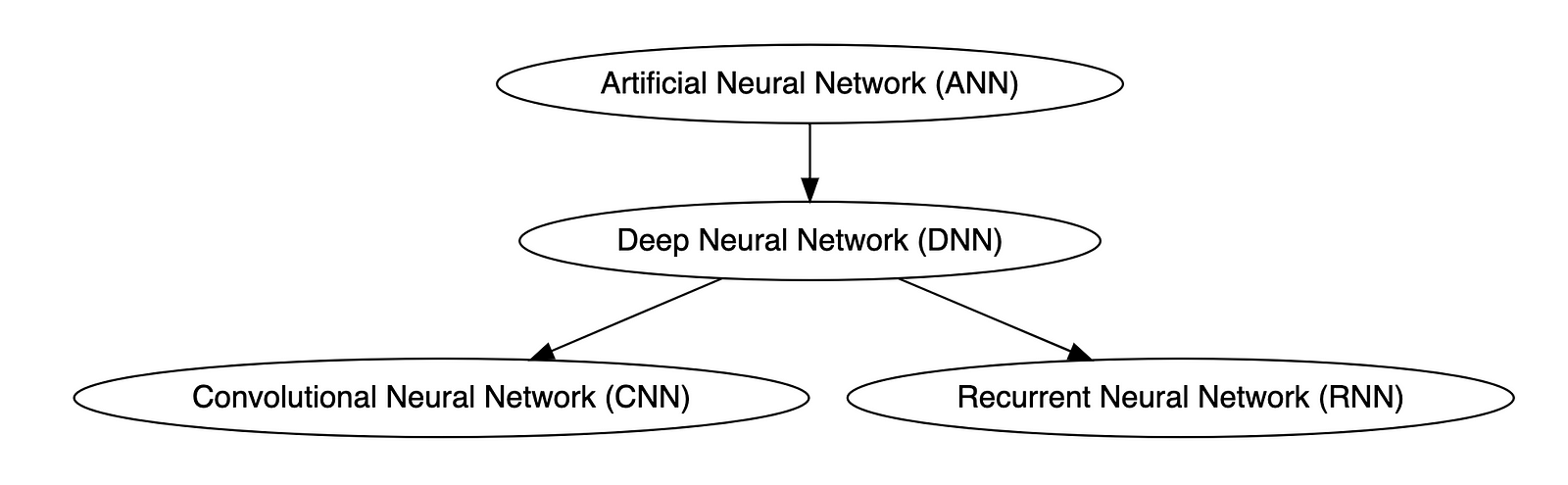
Below is a knowledge graph, created with OpenAI ChatGPT, showing the approximate relationships between the post’s terms.

Artificial General Intelligence (AGI)
According to the all-new Bing Chat, based on ChatGPT, artificial general intelligence (AGI) is the ability of an intelligent agent to understand or learn any intellectual task that human beings or other animals can. It is a primary goal of some artificial intelligence research and a common topic in science fiction and Futurism. According to Forbes, which also prompted ChatGPT, Artificial General Intelligence (AGI) refers to a theoretical type of artificial intelligence that possesses human-like cognitive abilities, such as the ability to learn, reason, solve problems, and communicate in natural language.
Eliezer Yudkowsky is an American researcher, writer, and philosopher on the topic of AI. The podcast Eliezer Yudkowsky: Dangers of AI and the End of Human Civilization, by prominent MIT Research Scientist Lex Fridman, explores various aspects of artificial general intelligence against the backdrop of the recent release of OpenAI’s GPT-4.
Artificial Intelligence (AI)
According to the Brookings Institute, AI is generally thought to refer to machines that respond to stimulation consistent with traditional responses from humans, given the human capacity for contemplation, judgment, and intention. Similarly, according to the U.S. Department of State, the term artificial intelligence refers to a machine-based system that can, for a given set of human-defined objectives, make predictions, recommendations, or decisions influencing real or virtual environments.

ChatGPT
ChatGPT, according to ChatGPT, is a large language model developed by OpenAI. I was trained on a massive dataset of human-written text using a deep neural network (DNN) architecture called GPT (Generative Pre-trained Transformer). Its purpose is to generate human-like responses to questions and prompts, engage in conversations, and perform various language-related tasks. It is a virtual assistant capable of understanding and generating natural language.
DALL·E
According to Wikipedia, DALL·E is a deep learning model developed by OpenAI to generate digital images from natural language descriptions, called prompts. DALL·E is a portmanteau of the names of the animated robot Pixar character WALL-E and the Spanish surrealist artist Salvador Dalí. According to OpenAI, DALL·E is an AI system that can create realistic images and art from a description in natural language. OpenAI introduced DALL·E in January 2021. One year later, in April 2022, they announced their newest system, DALL·E 2, which generates more realistic and accurate images with 4x greater resolution. DALL·E 2 can create original, realistic images and art from a text description. It can combine concepts, attributes, and styles.
Deep Learning (DL)
According to IBM, deep learning is a subset of machine learning (ML), which is essentially a neural network with three or more layers. These neural networks attempt to simulate the behavior of the human brain — albeit far from matching its ability — allowing it to “learn” from large amounts of data. While a neural network with a single layer can still make approximate predictions, additional hidden layers can help to optimize and refine for accuracy.
Generative AI
According to Wikipedia, generative artificial intelligence (AI), aka generative AI, is a type of AI system capable of generating text, images, or other media in response to prompts. Generative AI systems use generative models such as large language models (LLMs) to statistically sample new data based on the training data set used to create them.
Generative Pre-trained Transformer (GPT)
According to ChatGPT, Generative Pre-trained Transformer (GPT) is a deep learning architecture used for natural language processing (NLP) tasks, such as text generation, summarization, and question-answering. It uses a transformer neural network architecture with a self-attention mechanism, allowing the model to understand each word’s context in a sentence or text. The success of GPT models lies in their ability to generate natural-sounding and coherent text similar to human-written language. The term “pre-trained” refers to the fact that the model is trained on large amounts of unlabeled text data, such as books or web pages, to learn general language patterns and features, before being fine-tuned on smaller labeled datasets for specific tasks.
According to ZDNET, GPT-4, announced on March 14, 2023, is the newest version of OpenAI’s language model systems. Its previous version, GPT 3.5, powered the company’s wildly popular ChatGPT chatbot when it launched in November 2022. According to OpenAI, GPT-4 is the latest milestone in OpenAI’s effort to scale up deep learning. GPT-4 is a large multimodal model (accepting image and text inputs, emitting text outputs) that, while less capable than humans in many real-world scenarios, exhibits human-level performance on various professional and academic benchmarks.
Intelligence Amplification
According to Wikipedia, intelligence amplification (IA) (aka cognitive augmentation, machine-augmented intelligence, or enhanced intelligence) refers to the effective use of information technology in augmenting human intelligence. Similarly, Harvard Business Review describes intelligence amplification as the use of technology to augment human intelligence. And a paradigm shift is on the horizon, where new devices will offer less intrusive, more intuitive ways to amplify our intelligence.
In his latest book, Impromptu: Amplifying Our Humanity Through AI, co-authored by ChatGPT-4, Greylock general partner Reid Hoffman discusses the subject of intelligence amplification and AI’s ability to amplify human ability. The topic was also explored in Hoffman’s interview with OpenAI CEO Sam Altman on Greylock’s podcast series AI Field Notes.
Large Language Model (LLM)
According to Wikipedia, a large language model (LLM) is a language model consisting of a neural network with many parameters (typically billions of weights or more), trained on large quantities of unlabelled text using self-supervised learning. Though the term large language model has no formal definition, it often refers to deep learning models having a parameter count on the order of billions or more.
Machine Learning (ML)
According to MIT, machine learning (ML) is a subfield of artificial intelligence, which is broadly defined as the capability of a machine to imitate intelligent human behavior. Artificial intelligence systems are used to perform complex tasks in a way that is similar to how humans solve problems. The function of a machine learning system can be descriptive, meaning that the system uses the data to explain what happened; predictive, meaning the system uses the data to predict what will happen; or prescriptive, meaning the system will use the data to make suggestions about what action to take.
Neural Network
According to MathWorks, a neural network (aka artificial neural network or ANN) is an adaptive system that learns by using interconnected nodes or neurons in a layered structure that resembles a human brain. A neural network can learn from data to be trained to recognize patterns, classify data, and forecast future events. Similarly, according to AWS, a neural network is a method in artificial intelligence that teaches computers to process data in a way that is inspired by the human brain. It is a type of machine learning process called deep learning that uses interconnected nodes or neurons in a layered structure that resembles the human brain. It creates an adaptive system that computers use to learn from their mistakes and improve continuously.
Types of Neural Networks
Deep neural networks (DNNs) are improved versions of conventional artificial neural networks (ANNs) with multiple layers. While ANNs consist of one or two hidden layers to process data, DNNs contain multiple layers between the input and output layers. Convolutional neural networks (CNNs) are another kind of DNN. CNNs have a convolution layer, which uses filters to convolve an area of input data into a smaller area, detecting important or specific parts within the area. Recurrent neural networks (RNNs) can be considered a type of DNN. DNNs are neural networks with multiple layers between the input and output layers. RNNs can have multiple layers and can be used to process sequential data, making them a type of DNN.
OpenAI
OpenAI is a San Francisco-based AI research and deployment company whose mission is to “ensure that artificial general intelligence benefits all of humanity.” According to Wikipedia, OpenAI was founded in 2015 by current CEO Sam Altman, Greylock general partner Reid Hoffman, Y Combinator founding partner Jessica Livingston, Elon Musk, Ilya Sutskever, Peter Thiel, and others. OpenAI’s current products include GPT-4, DALL·E 2, Whisper, ChatGPT, and OpenAI Codex.

Prompt Engineering
According to Cohere, prompting (aka prompt engineering) is at the heart of working with LLMs. The prompt provides context for the text we want the model to generate. The prompts we create can be anything from simple instructions to more complex pieces of text, and they are used to encourage the model to produce a specific type of output. Cohere’s Generative AI with Cohere blog post series is an excellent resource on the topic of Prompting. Similarly, according to Dataconomy, using prompts to get the desired result from an AI tool is known as AI prompt engineering. A prompt can be a statement or a block of code, but it can also just be a string of words. Similar to how you may prompt a person as a starting point for writing an essay, you can use prompts to teach an AI model to produce the desired results when given a specific task.
Reinforcement Learning with Human Feedback (RLHF)
According to Scale AI in their blog, Why is ChatGPT so good?, instead of simply predicting the next word(s), large language models (LLMs) can now follow human instructions and provide useful responses. These advancements are made possible by fine-tuning them with specialized instruction datasets and a technique called reinforcement learning with human feedback (RLHF). Similarly, according to Hugging Face, RLHF (aka RL from human preferences) uses methods from reinforcement learning to directly optimize LLMs with human feedback. RLHF has enabled language models to begin to align a model trained on a geprogneral corpus of text data to that of complex human values.
Ready for More?
Mastered all the terminology, ready for more? Here are some additional generative AI terms for you to learn:
- Alignment (AI Alignment, Aligned AI)
- Attention (Self-attention)
- Backpropagation
- Embeddings
- Foundational Model
- Next-Token Predictors
- Parameter
- Reinforcement Learning (RL)
- Self-Supervised Learning (SSL)
- Temperature
- Tokenization
- Transformer
- Vector
- Weight
🔔 To keep up with future content, follow Gary Stafford on LinkedIn.
This blog represents my viewpoints and not those of my employer, Amazon Web Services (AWS). All product names, logos, and brands are the property of their respective owners.
Developing a Multi-Account AWS Environment Strategy
Posted by Gary A. Stafford in AWS, Cloud, DevOps, Enterprise Software Development, Technology Consulting on March 11, 2023
Explore twelve common patterns for developing an effective and efficient multi-account AWS environment strategy

Introduction
Every company is different: its organizational structure, the length of time it has existed, how fast it has grown, the industries it serves, its product and service diversity, public or private sector, and its geographic footprint. This uniqueness is reflected in how it organizes and manages its Cloud resources. Just as no two organizations are exactly alike, the structure of their AWS environments is rarely identical.
Some organizations successfully operate from a single AWS account, while others manage workloads spread across dozens or even hundreds of accounts. The volume and purpose of an organization’s AWS accounts are a result of multiple factors, including length of time spent on AWS, Cloud maturity, organizational structure and complexity, sectors, industries, and geographies served, product and service mix, compliance and regulatory requirements, and merger and acquisition activity.
“By design, all resources provisioned within an AWS account are logically isolated from resources provisioned in other AWS accounts, even within your own AWS Organizations.” (AWS)
Working with industry peers, the AWS community, and a wide variety of customers, one will observe common patterns for how organizations separate environments and workloads using AWS accounts. These patterns form an AWS multi-account strategy for operating securely and reliably in the Cloud at scale. The more planning an organization does in advance to develop a sound multi-account strategy, the less the burden that is required to manage changes as the organization grows over time.
The following post will explore twelve common patterns for effectively and efficiently organizing multiple AWS accounts. These patterns do not represent an either-or choice; they are designed to be purposefully combined to form a multi-account AWS environment strategy for your organization.
Patterns
- Pattern 1: Single “Uber” Account
- Pattern 2: Non-Prod/Prod Environments
- Pattern 3: Upper/Lower Environments
- Pattern 4: SDLC Environments
- Pattern 5: Major Workload Separation
- Pattern 6: Backup
- Pattern 7: Sandboxes
- Pattern 8: Centralized Management and Governance
- Pattern 9: Internal/External Environments
- Pattern 10: PCI DSS Workloads
- Pattern 11: Vendors and Contractors
- Pattern 12: Mergers and Acquisitions
Patterns 1–8 are progressively more mature multi-account strategies, while Patterns 9–12 represent special use cases for supplemental accounts.
Multi-Account Advantages
According to AWS’s whitepaper, Organizing Your AWS Environment Using Multiple Accounts, the benefits of using multiple AWS accounts include the following:
- Group workloads based on business purpose and ownership
- Apply distinct security controls by environment
- Constrain access to sensitive data (including compliance and regulation)
- Promote innovation and agility
- Limit the scope of impact from adverse events
- Support multiple IT operating models
- Manage costs (budgeting and cost attribution)
- Distribute AWS Service Quotas (fka limits) and API request rate limits
As we explore the patterns for organizing your AWS accounts, we will see how and to what degree each of these benefits is demonstrated by that particular pattern.
AWS Control Tower
Discussions about AWS multi-account environment strategies would not be complete without mentioning AWS Control Tower. According to the documentation, “AWS Control Tower offers a straightforward way to set up and govern an AWS multi-account environment, following prescriptive best practices.” AWS Control Tower includes Landing zone, described as “a well-architected, multi-account environment based on security and compliance best practices.”
AWS Control Tower is prescriptive in the Shared accounts it automatically creates within its AWS Organizations’ organizational units (OUs). Shared accounts created by AWS Control Tower include the Management, Log Archive, and Audit accounts. The previous standalone AWS service, AWS Landing Zone, maintained slightly different required accounts, including Shared Services, Log Archive, Security, and optional Network accounts. Although prescriptive, AWS Control Tower is also flexible and relatively unopinionated regarding the structure of Member accounts. Member accounts can be enrolled or unenrolled in AWS Control Tower.
You can decide whether or not to implement AWS Organizations or AWS Control Tower to set up and govern your AWS multi-account environment. Regardless, you will still need to determine how to reflect your organization’s unique structure and requirements in the purpose and quantity of the accounts you create within your AWS environment.
Common Multi-Account Patterns
While working with peers, community members, and a wide variety of customers, I regularly encounter the following twelve patterns for organizing AWS accounts. As noted earlier, these patterns do not represent an either-or choice; they are designed to be purposefully combined to form a multi-account AWS environment strategy for your organization.
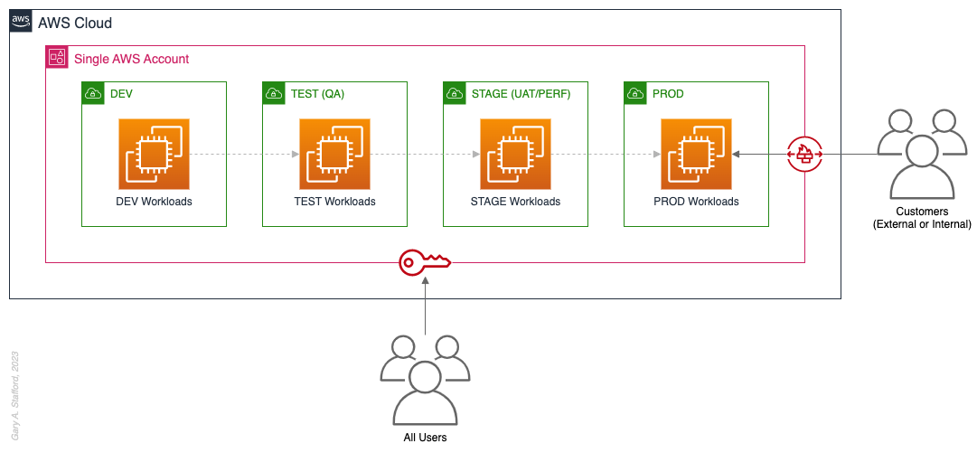
Pattern 1: Single “Uber” Account
Organizations that effectively implement Pattern 1: Single “Uber” Account organize and separate environments and workloads at the sub-account level. They often use Amazon Virtual Private Cloud (Amazon VPC), an AWS account-level construct, to organize and separate environments and workloads. They may also use Subnets (VPC-level construct) or AWS Regions and Availability Zones to further organize and separate environments and workloads.
Pros
- Few, if any, significant advantages, especially for customer-facing workloads
Cons
- Decreased ability to limit the scope of impact from adverse events (widest blast radius)
- If the account is compromised, then all the organization’s workloads and data, possibly the entire organization, are potentially compromised (e.g., Ransomware attacks such as Encryptors, Lockers, and Doxware)
- Increased risk that networking or security misconfiguration could lead to unintended access to sensitive workloads and data
- Increased risk that networking, security, or resource management misconfiguration could lead to broad or unintended impairment of all workloads
- Decreased ability to perform team-, environment-, and workload-level budgeting and cost attribution
- Increased risk of resource depletion (soft and hard service quotas)
- Reduced ability to conduct audits and demonstrate compliance
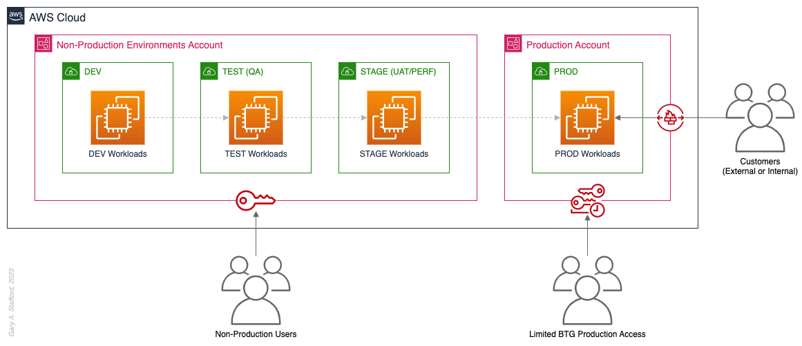
Pattern 2: Non-Prod/Prod Environments
Organizations that effectively implement Pattern 2: Non-Prod/Prod Environments organize and separate non-Production workloads from Production (PROD) workloads using separate AWS accounts. Most often, they use Amazon VPCs within the non-Production account to separate workloads or Software Development Lifecycle (SDLC) environments, most often Development (DEV), Testing (TEST) or Quality Assurance (QA), and Staging (STAGE). Alternatively, these environments might also be designated as “N-1” (previous release), “N” (current release), “N+1” (next release), “N+2” (in development), and so forth, based on the currency of that version of that workload.
In some organizations, the Staging environment is used for User Acceptance Testing (UAT), performance (PERF) testing, and load testing before releasing workloads to Production. While in other organizations, STAGE, UAT, and PERF are each treated as separate environments at the account or VPC level.
Isolating Production workloads into their own account(s) and strictly limiting access to those workloads represents a significant first step in improving the overall maturity of your multi-account AWS environment strategy.
Pros
- Limits the scope of impact on Production as a result of adverse non-Production events (narrower blast radius)
- Logical separation and security of Production workloads and data
- Tightly control and limit access to Production, including the use of Break-the-Glass procedures (aka Break-glass or BTG); draws its name from “breaking the glass to pull a fire alarm”
- Eliminate the risk that non-Production networking or security misconfiguration could lead to unintended access to sensitive Production workloads and data
- Eliminate the chance that non-Production networking, security, or resource management misconfiguration could lead to broad or unintended impairment of Production workloads
- Conduct audits and demonstrate compliance with Production workloads
Cons
- If the Production account is compromised, then all the organization’s customer-facing workloads and data are potentially compromised
- Decreased ability to perform team-, environment-, and workload-level budgeting and cost attribution in the shared non-Production environment
- Increased risk of resource depletion (soft and hard service quotas) in the non-Production environment account
Pattern 3: Upper/Lower Environments
The next pattern, Pattern 3: Upper/Lower Environments, is a finer-grain variation of Pattern 2. With Pattern 3, we split all “Lower” environments into a single account and each “Upper” environment into its own account. In the software development process, initial environments, such as CI/CD for automated testing of code and infrastructure, Development, Test, UAT, and Performance, are called “Lower” environments. Conversely, later environments, such as Staging, Production, and even Disaster Recovery (DR), are called “Upper” environments. Upper environments typically require isolation for stability during testing or security for Production workloads and sensitive data.
Often, courser-grain patterns like Patterns 1–3 are carryovers from more traditional on-premises data centers, where compute, storage, network, and security resources were more constrained. Although these patterns can be successfully reproduced in the Cloud, they may not be optimal compared to more “cloud native” patterns, which provide improved separation of concerns.

Pros
- Limits the scope of impact on individual Upper environments as a result of adverse Lower environment events (narrower blast radius)
- Increased stability of Staging environment for critical UAT, performance, and load testing
- Logical separation and security of Production workloads and data
- Tightly control and limit access to Production, including the use of BTG
- Eliminate the risk that non-Production networking or security misconfiguration could lead to unintended access to sensitive Production workloads and data
- Eliminate the chance that non-Production networking, security, or resource management misconfiguration could lead to broad or unintended impairment of Production workloads
- Conduct audits and demonstrate compliance with Production workloads
Cons
- If the Production account is compromised, then all the organization’s customer-facing workloads and data are potentially compromised (e.g., Ransomware attack)
- Decreased ability to perform team-, environment-, and workload-level budgeting and cost attribution in the shared Lower environment
- Increased risk of resource depletion (soft and hard service quotas) in the Lower environment account
Pattern 4: SDLC Environments
The next pattern, Pattern 4: SDLC Environments, is a finer-grain variation of Pattern 3. With Pattern 4, we gain complete separation of each SDLC environment into its own AWS account. Using AWS services like AWS IAM Identity Center (fka AWS SSO), the Security team can enforce least-privilege permissions at an AWS Account level to individual groups of users, such as Developers, Testers, UAT, and Performance testers.
Based on my experience, Pattern 4 represents the minimal level of workload separation an organization should consider when developing its multi-account AWS environment strategy. Although Pattern 4 has a number of disadvantages, when combined with subsequent patterns and AWS best practices, this pattern begins to provide a scalable foundation for an organization’s growing workload portfolio.

Patterns, such as Pattern 4, not only apply to traditional software applications and services. These patterns can be applied to data analytics, AI/ML, IoT, media services, and similar workloads where separation of environments is required.

Pros
- Limits the scope of impact on one SDLC environment as a result of adverse events in another environment (narrower blast radius)
- Logical separation and security of Production workloads and data
- Increased stability of each SDLC environment
- Tightly control and limit access to Production, including the use of BTG
- Reduced risk that non-Production networking or security misconfiguration could lead to unintended access to sensitive Production workloads and data
- Reduced risk that non-Production networking, security, or resource management misconfiguration could lead to broad or unintended impairment of Production workloads
- Conduct audits and demonstrate compliance with Production workloads
- Increased ability to perform budgeting and cost attribution for each SDLC environment
- Reduced risk of resource depletion (soft and hard service limits) and IP conflicts and exhaustion within any single SDLC environment
Cons
- All workloads for each SDLC environment run within a single account, including Production, increasing the potential scope of impact from adverse events within that environment’s account
- If the Production account is compromised, then all the organization’s customer-facing workloads and data are potentially compromised
- Decreased ability to perform workload-level budgeting and cost attribution
Pattern 5: Major Workload Separation
The next pattern, Pattern 5: Major Workload Separation, is a finer-grain variation of Pattern 4. With Pattern 5, we separate each significant workload into its own separate SDLC environment account. The security team can enforce fine-grain least-privilege permissions at an AWS Account level to individual groups of users, such as Developers, Testers, UAT, and Performance testers, by their designated workload(s).
Pattern 5 has several advantages over the previous patterns. In addition to the increased workload-level security and reliability benefits, Pattern 5 can be particularly useful for organizations that operate significantly different technology stacks and specialized workloads, particularly at scale. Different technology stacks and specialized workloads often each have their own unique development, testing, deployment, and support processes. Isolating these types of workloads will help facilitate the support of multiple IT operating models.

Pros
- Limits the scope of impact on an individual workload as a result of adverse events from another workload or SDLC environment (narrowest blast radius)
- Increased ability to perform team-, environment-, and workload-level budgeting and cost attribution
Cons
- If the Production account is compromised, then all the organization’s customer-facing workloads and data are potentially compromised (e.g., Ransomware attack)
Pattern 6: Backup
In the earlier patterns, we mentioned that if the Production account were compromised, all the organization’s customer-facing workloads and data could be compromised. According to TechTarget, 2022 was a breakout year for Ransomware attacks. According to the US government’s CISA.gov website, “Ransomware is a form of malware designed to encrypt files on a device, rendering any files and the systems that rely on them unusable. Malicious actors then demand ransom in exchange for decryption.”
According to AWS best practices, one of the recommended preparatory actions to protect and recover from Ransomware attacks is backing up data to an alternate account using tools such as AWS Backup and an AWS Backup vault. Solutions such as AWS Backup protect and restore data regardless of how it was made inaccessible.
In Pattern 6: Backup, we create one or more Backup accounts to protect against unintended data loss or account compromise. In the example below, we have two Backup accounts, one for Production data and one for all non-Production data.

Pros
- If the Production account is compromised (e.g., Ransomware attacks such as Encryptors, Lockers, and Doxware), there are secure backups of data stored in a separate account, which can be used to restore or recreate the Production environment
Cons
- Few, if any, significant disadvantages when combined with previous patterns and AWS best-practices
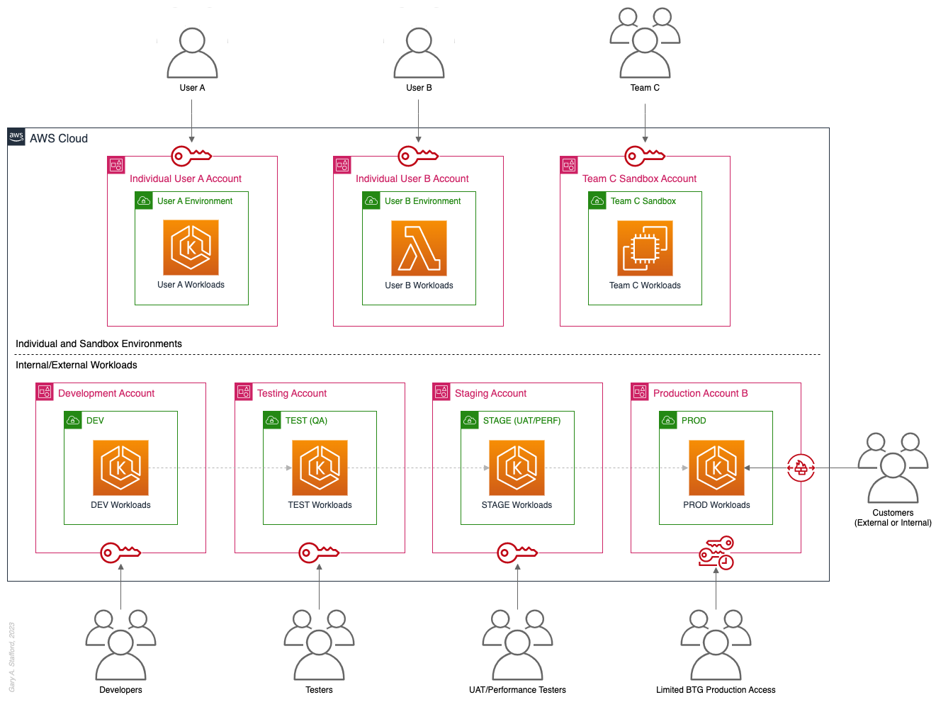
Pattern 7: Sandboxes
The following pattern, Pattern 7: Sandboxes, supplements the previous patterns, designed to address the needs of an organization to allow individual users and teams to learn, build, experiment, and innovate on AWS without impacting the larger organization’s AWS environment. To quote the AWS blog, Best practices for creating and managing sandbox accounts in AWS, “Many organizations need another type of environment, one where users can build and innovate with AWS services that might not be permitted in production or development/test environments because controls have not yet been implemented.” Further, according to TechTarget, “a Sandbox is an isolated testing environment that enables users to run programs or open files without affecting the application, system, or platform on which they run.”
Due to the potential volume of individual user and team accounts, sometimes referred to as Sandbox accounts, mature infrastructure automation practices, cost controls, and self-service provisioning and de-provisioning of Sandbox accounts are critical capabilities for the organization.
Pros
- Allow individual users and teams to learn, build, experiment, and innovate on AWS without impacting the rest of the organization’s AWS environment
Cons
- Without mature automation practices, cost controls, and self-service capabilities, managing multiple individual and team Sandbox accounts can become unwieldy and costly
Pattern 8: Centralized Management and Governance
We discussed AWS Control Tower at the beginning of this post. AWS Control Tower is prescriptive in creating Shared accounts within its AWS Organizations’ organizational units (OUs), including the Management, Log Archive, and Audit accounts. AWS encourages using AWS Control Tower to orchestrate multiple AWS accounts and services on your behalf while maintaining your organization’s security and compliance needs.
As exemplified in Pattern 8: Centralized Management and Governance, many organizations will implement centralized management whether or not they decide to implement AWS Control Tower. In addition to the Management account (payer account, fka master account), organizations often create centralized logging accounts, and centralized tooling (aka Shared services) accounts for functions such as CI/CD, IaC provisioning, and deployment. Another common centralized management account is a Security account. Organizations use this account to centralize the monitoring, analysis, notification, and automated mitigation of potential security issues within their AWS environment. The Security accounts will include services such as Amazon Detective, Amazon Inspector, Amazon GuardDuty, and AWS Security Hub.

Pros
- Increased ability to manage and maintain multiple AWS accounts with fewer resources
- Reduced duplication of management resources across accounts
- Increased ability to use automation and improve the consistency of processes and procedures across multiple accounts
Cons
- Few, if any, significant disadvantages when combined with previous patterns and AWS best-practices
Pattern 9: Internal/External Environments
The next pattern, Pattern 9: Internal/External Environments, focuses on organizations with internal operational systems (aka Enterprise systems) in the Cloud and customer-facing workloads. Pattern 9 separates internal operational systems, platforms, and workloads from external customer-facing workloads. For example, an organization’s divisions and departments, such as Sales and Marketing, Finance, Human Resources, and Manufacturing, are assigned their own AWS account(s). Pattern 9 allows the Security team to ensure that internal departmental or divisional users are isolated from users who are responsible for developing, testing, deploying, and managing customer-facing workloads.
Note that the diagram for Pattern 9 shows remote users who access AWS End User Computing (EUC) services or Virtual Desktop Infrastructure (VDI), such as Amazon WorkSpaces and Amazon AppStream 2.0. In this example, remote workers have secure access to EUC services provisioned in a separate AWS account, and indirectly, internal systems, platforms, and workloads.

Pros
- Separation of internal operational systems, platforms, and workloads from external customer-facing workloads
Cons
- Few, if any, significant disadvantages when combined with previous patterns and AWS best-practices
Pattern 10: PCI DSS Workloads
The next pattern, Pattern 10: PCI DSS Workloads, is a variation of previous patterns, which assumes the existence of Payment Card Industry Data Security Standard (PCI DSS) workloads and data. According to the AWS, “PCI DSS applies to entities that store, process, or transmit cardholder data (CHD) or sensitive authentication data (SAD), including merchants, processors, acquirers, issuers, and service providers. The PCI DSS is mandated by the card brands and administered by the Payment Card Industry Security Standards Council.”
According to AWS’s whitepaper, Architecting for PCI DSS Scoping and Segmentation on AWS, “By design, all resources provisioned within an AWS account are logically isolated from resources provisioned in other AWS accounts, even within your own AWS Organizations. Using an isolated account for PCI workloads is a core best practice when designing your PCI application to run on AWS.” With Pattern 10, we separate non-PCI DSS and PCI DSS Production workloads and data. The assumption is that only Production contains PCI DSS data. Data in lower environments is synthetically generated or sufficiently encrypted, masked, obfuscated, or tokenized.
Note that the diagram for Pattern 10 shows Administrators. Administrators with different spans of responsibility and access are present in every pattern, whether specifically shown or not.

Pros
- Increased ability to meet compliance requirements by separating non-PCI DSS and PCI DSS Production workloads
Cons
- Few, if any, significant disadvantages when combined with previous patterns and AWS best-practices
Pattern 11: Vendors and Contractors
The next pattern, Pattern 11: Vendors and Contractors, is focused on organizations that employ contractors or use third-party vendors who provide products and services that interact with their AWS-based environment. Like Pattern 10, Pattern 11 allows the Security team to ensure that contractor and vendor-based systems’ access to internal systems and customer-facing workloads is tightly controlled and auditable.
Vendor-based products and services are often deployed within an organization’s AWS environment without external means of ingress or egress. Alternatively, a vendor’s product or service may have a secure means of ingress from or egress to external endpoints. Such is the case with some SaaS products, which ship an organization’s data to an external aggregator for analytics or a security vendor’s product that pre-filters incoming data, external to the organization’s AWS environment. Using separate AWS accounts can improve an organization’s security posture and mitigate the risk of adverse events on the organization’s overall AWS environment.

Pros
- Ensure access to internal systems and customer-facing workloads by contractors and vendor-based systems is tightly controlled and auditable
Cons
- Few, if any, significant disadvantages when combined with previous patterns and AWS best-practices
Pattern 12: Mergers and Acquisitions
The next pattern, Pattern 12: Mergers and Acquisitions, is focused on managing the integration of external AWS accounts as a result of a merger or acquisition. This is a common occurrence, but the exact details of how best to handle the integration of two or more integrations depend on several factors. Factors include the required level of integration, for example, maintaining separate AWS Organizations, maintaining different AWS accounts, or merging resources from multiple accounts. Other factors that might impact account structure include changes in ownership or payer of acquired accounts, existing acquired cost-savings agreements (e.g., EDPs, PPAs, RIs, and Savings Plans), and AWS Marketplace vendor agreements. Even existing authentication and authorization methods of the acquiree versus the acquirer (e.g., AWS IAM Identity Center, Microsoft Active Directory (AD), Azure AD, and external identity providers (IdP) like Okta or Auth0).
The diagram for Pattern 12 attempts to show a few different M&A account scenarios, including maintaining separate AWS accounts for the acquirer and acquiree (e.g., acquiree’s Manufacturing Division account). If desired, the accounts can be kept independent but managed within the acquirer’s AWS Organizations’ organization. The diagram also exhibits merging resources from the acquiree’s accounts into the acquirer’s accounts (e.g., Sales and Marketing accounts). Resources will be migrated or decommissioned, and the account will be closed.

Pros
- Maintain separation between an acquirer and an acquiree’s AWS accounts within a single organization’s AWS environment
- Potentially consolidate and maximize cost-saving advantages of volume-related financial agreements and vendor licensing
Cons
- Migrating workloads between different organizations, depending on their complexity, requires careful planning and testing
- Consolidating multiple authentication and authorization methods requires careful planning and testing to avoid improper privileges
- Consolidating and optimizing separate licensing and cost-saving agreements between multiple organizations requires careful planning and an in-depth understanding of those agreements
Multi-Account AWS Environment Example
You can form an efficient and effective multi-account strategy for your organization by purposefully combining multiple patterns. Below is an example of combining the features of several patterns: Major Workload Separation, Backup, Sandboxes, Centralized Management and Governance, Internal/External Environments, and Vendors and Contractors.
According to AWS, “You can use AWS Organizations’ organizational units (OUs) to group accounts together to administer as a single unit. This greatly simplifies the management of your accounts.” If you decide to use AWS Organizations, each set of accounts associated with a pattern could correspond to an OU: Major Workload A, Major Workload B, Sandboxes, Backups, Centralized Management, Internal Environments, Vendors, and Contractors.

Conclusion
This post taught us twelve common patterns for effectively and efficiently organizing your AWS accounts. Instead of an either-or choice, these patterns are designed to be purposefully combined to form a multi-account strategy for your organization. Having a sound multi-account strategy will improve your security posture, maintain compliance, decrease the impact of adverse events on your AWS environment, and improve your organization’s ability to safely and confidently innovate and experiment on AWS.
Recommended References
- Establishing Your Cloud Foundation on AWS (AWS Whitepaper)
- Organizing Your AWS Environment Using Multiple Accounts (AWS Whitepaper)
- Building a Cloud Operating Model (AWS Whitepaper)
- AWS Security Reference Architecture (AWS Prescriptive Guidance)
- AWS Security Maturity Model (AWS Whitepaper)
- AWS re:Invent 2022 — Best practices for organizing and operating on AWS (YouTube Video)
- AWS Break Glass Role (GitHub)
🔔 To keep up with future content, follow Gary Stafford on LinkedIn.
This blog represents my viewpoints and not those of my employer, Amazon Web Services (AWS). All product names, logos, and brands are the property of their respective owners.
Monolith to Microservices: Refactoring Relational Databases
Posted by Gary A. Stafford in Enterprise Software Development, SQL, Technology Consulting on April 14, 2022
Exploring common patterns for refactoring relational database models as part of a microservices architecture
Introduction
There is no shortage of books, articles, tutorials, and presentations on migrating existing monolithic applications to microservices, nor designing new applications using a microservices architecture. It has been one of the most popular IT topics for the last several years. Unfortunately, monolithic architectures often have equally monolithic database models. As organizations evolve from monolithic to microservices architectures, refactoring the application’s database model is often overlooked or deprioritized. Similarly, as organizations develop new microservices-based applications, they frequently neglect to apply a similar strategy to their databases.

The following post will examine several basic patterns for refactoring relational databases for microservices-based applications.
Terminology
Monolithic Architecture
A monolithic architecture is “the traditional unified model for the design of a software program. Monolithic, in this context, means composed all in one piece.” (TechTarget). A monolithic application “has all or most of its functionality within a single process or container, and it’s componentized in internal layers or libraries” (Microsoft). A monolith is usually built, deployed, and upgraded as a single unit of code.
Microservices Architecture
A microservices architecture (aka microservices) refers to “an architectural style for developing applications. Microservices allow a large application to be separated into smaller independent parts, with each part having its own realm of responsibility” (Google Cloud).
According to microservices.io, the advantages of microservices include:
- Highly maintainable and testable
- Loosely coupled
- Independently deployable
- Organized around business capabilities
- Owned by a small team
- Enables rapid, frequent, and reliable delivery
- Allows an organization to [more easily] evolve its technology stack
Database
A database is “an organized collection of structured information, or data, typically stored electronically in a computer system” (Oracle). There are many types of databases. The most common database engines include relational, NoSQL, key-value, document, in-memory, graph, time series, wide column, and ledger.
PostgreSQL
In this post, we will use PostgreSQL (aka Postgres), a popular open-source object-relational database. A relational database is “a collection of data items with pre-defined relationships between them. These items are organized as a set of tables with columns and rows. Tables are used to hold information about the objects to be represented in the database” (AWS).
Amazon RDS for PostgreSQL
We will use the fully managed Amazon RDS for PostgreSQL in this post. Amazon RDS makes it easy to set up, operate, and scale PostgreSQL deployments in the cloud. With Amazon RDS, you can deploy scalable PostgreSQL deployments in minutes with cost-efficient and resizable hardware capacity. In addition, Amazon RDS offers multiple versions of PostgreSQL, including the latest version used for this post, 14.2.
The patterns discussed here are not specific to Amazon RDS for PostgreSQL. There are many options for using PostgreSQL on the public cloud or within your private data center. Alternately, you could choose Amazon Aurora PostgreSQL-Compatible Edition, Google Cloud’s Cloud SQL for PostgreSQL, Microsoft’s Azure Database for PostgreSQL, ElephantSQL, or your own self-manage PostgreSQL deployed to bare metal servers, virtual machine (VM), or container.
Database Refactoring Patterns
There are many ways in which a relational database, such as PostgreSQL, can be refactored to optimize efficiency in microservices-based application architectures. As stated earlier, a database is an organized collection of structured data. Therefore, most refactoring patterns reorganize the data to optimize for an organization’s functional requirements, such as database access efficiency, performance, resilience, security, compliance, and manageability.
The basic building block of Amazon RDS is the DB instance, where you create your databases. You choose the engine-specific characteristics of the DB instance when you create it, such as storage capacity, CPU, memory, and EC2 instance type on which the database server runs. A single Amazon RDS database instance can contain multiple databases. Those databases contain numerous object types, including tables, views, functions, procedures, and types. Tables and other object types are organized into schemas. These hierarchal constructs — instances, databases, schemas, and tables — can be arranged in different ways depending on the requirements of the database data producers and consumers.

Sample Database
To demonstrate different patterns, we need data. Specifically, we need a database with data. Conveniently, due to the popularity of PostgreSQL, there are many available sample databases, including the Pagila database. I have used it in many previous articles and demonstrations. The Pagila database is available for download from several sources.

The Pagila database represents a DVD rental business. The database is well-built, small, and adheres to a third normal form (3NF) database schema design. The Pagila database has many objects, including 1 schema, 15 tables, 1 trigger, 7 views, 8 functions, 1 domain, 1 type, 1 aggregate, and 13 sequences. Pagila’s tables contain between 2 and 16K rows.
Pattern 1: Single Schema
Pattern 1: Single Schema is one of the most basic database patterns. There is one database instance containing a single database. That database has a single schema containing all tables and other database objects.

As organizations begin to move from monolithic to microservices architectures, they often retain their monolithic database architecture for some time.

Frequently, the monolithic database’s data model is equally monolithic, lacking proper separation of concerns using simple database constructs such as schemas. The Pagila database is an example of this first pattern. The Pagila database has a single schema containing all database object types, including tables, functions, views, procedures, sequences, and triggers.
To create a copy of the Pagila database, we can use pg_restore to restore any of several publically available custom-format database archive files. If you already have the Pagila database running, simply create a copy with pg_dump.
Below we see the table layout of the Pagila database, which contains the single, default public schema.
-----------+----------+--------+------------
 Instance  | Database | Schema | Table
-----------+----------+--------+------------
 postgres1 | pagila   | public | actor
 postgres1 | pagila   | public | address
 postgres1 | pagila   | public | category
 postgres1 | pagila   | public | city
 postgres1 | pagila   | public | country
 postgres1 | pagila   | public | customer
 postgres1 | pagila   | public | film
 postgres1 | pagila   | public | film_actor
 postgres1 | pagila   | public | film_category
 postgres1 | pagila   | public | inventory
 postgres1 | pagila   | public | language
 postgres1 | pagila   | public | payment
 postgres1 | pagila   | public | rental
 postgres1 | pagila   | public | staff
 postgres1 | pagila   | public | store
Using a single schema to house all tables, especially the public schema is generally considered poor database design. As a database grows in complexity, creating, organizing, managing, and securing dozens, hundreds, or thousands of database objects, including tables, within a single schema becomes impossible. For example, given a single schema, the only way to organize large numbers of database objects is by using lengthy and cryptic naming conventions.
Public Schema
According to the PostgreSQL docs, if tables or other object types are created without specifying a schema name, they are automatically assigned to the default public schema. Every new database contains a public schema. By default, users cannot access any objects in schemas they do not own. To allow that, the schema owner must grant the USAGE privilege on the schema. by default, everyone has CREATE and USAGE privileges on the schema public. These default privileges enable all users to connect to a given database to create objects in its public schema. Some usage patterns call for revoking that privilege, which is a compelling reason not to use the public schema as part of your database design.
Pattern 2: Multiple Schemas
Separating tables and other database objects into multiple schemas is an excellent first step to refactoring a database to support microservices. As application complexity and databases naturally grow over time, schemas to separate functionality by business subdomain or teams will benefit significantly.
According to the PostgreSQL docs, there are several reasons why one might want to use schemas:
- To allow many users to use one database without interfering with each other.
- To organize database objects into logical groups to make them more manageable.
- Third-party applications can be put into separate schemas, so they do not collide with the names of other objects.
Schemas are analogous to directories at the operating system level, except schemas cannot be nested.

With Pattern 2, as an organization continues to decompose its monolithic application architecture to a microservices-based application, it could transition to a schema-per-microservice or similar level or organizational granularity.

Applying Domain-driven Design Principles
Domain-driven design (DDD) is “a software design approach focusing on modeling software to match a domain according to input from that domain’s experts” (Wikipedia). Architects often apply DDD principles to decompose a monolithic application into microservices. For example, a microservice or set of related microservices might represent a Bounded Context. In DDD, a Bounded Context is “a description of a boundary, typically a subsystem or the work of a particular team, within which a particular model is defined and applicable.” (hackernoon.com). Examples of Bounded Context might include Sales, Shipping, and Support.
One technique to apply schemas when refactoring a database is to mirror the Bounded Contexts, which reflect the microservices. For each microservice or set of closely related microservices, there is a schema. Unfortunately, there is no absolute way to define the Bounded Contexts of a Domain, and henceforth, schemas to a database. It depends on many factors, including your application architecture, features, security requirements, and often an organization’s functional team structure.
Reviewing the purpose of each table in the Pagila database and their relationships to each other, we could infer Bounded Contexts, such as Films, Stores, Customers, and Sales. We can represent these Bounded Contexts as schemas within the database as a way to organize the data. The individual tables in a schema mirror DDD concepts, such as aggregates, entities, or value objects.
As shown below, the tables of the Pagila database have been relocated into six new schemas: common, customers, films, sales, staff, and stores. The common schema contains tables with address data references tables in several other schemas. There are now no tables left in the public schema. We will assume other database objects (e.g., functions, views, and triggers) have also been moved and modified if necessary to reflect new table locations.
-----------+----------+-----------+---------------
 Instance  | Database | Schema    | Table
-----------+----------+-----------+---------------
 postgres1 | pagila   | common    | address
 postgres1 | pagila   | common    | city
 postgres1 | pagila   | common    | country
-----------+----------+-----------+---------------
 postgres1 | pagila   | customers | customer
-----------+----------+-----------+---------------
 postgres1 | pagila   | films     | actor
 postgres1 | pagila   | films     | category
 postgres1 | pagila   | films     | film
 postgres1 | pagila   | films     | film_actor
 postgres1 | pagila   | films     | film_category
 postgres1 | pagila   | films     | language
-----------+----------+-----------+---------------
 postgres1 | pagila   | sales     | payment
 postgres1 | pagila   | sales     | rental
-----------+----------+-----------+---------------
 postgres1 | pagila   | staff     | staff
-----------+----------+-----------+---------------
 postgres1 | pagila   | stores    | inventory
 postgres1 | pagila   | stores    | store
By applying schemas, we align tables and other database objects to individual microservices or functional teams that own the microservices and the associated data. Schemas allow us to apply fine-grain access control over objects and data within the database more effectively.

Refactoring other Database Objects
Typically with psql, when moving tables across schemas using an ALTER TABLE...SET SCHEMA... SQL statement, objects such as database views will be updated to the table’s new location. For example, take Pagila’s sales_by_store view. Note the schemas have been automatically updated for multiple tables from their original location in the public schema. The view was also moved to the sales schema.
Splitting Table Data Across Multiple Schemas
When refactoring a database, you may have to split data by replicating table definitions across multiple schemas. Take, for example, Pagila’s address table, which contains the addresses of customers, staff, and stores. The customers.customer, stores.staff, and stores.store all have foreign key relationships with the common.address table. The address table has a foreign key relationship with both the city and country tables. Thus for convenience, the address, city, and country tables were all placed into the common schema in the example above.
Although, at first, storing all the addresses in a single table might appear to be sound database normalization, consider the risks of having the address table’s data exposed. The store addresses are not considered sensitive data. However, the home addresses of customers and staff are likely considered sensitive personally identifiable information (PII). Also, consider as an application evolves, you may have fields unique to one type of address that does not apply to other categories of addresses. The table definitions for a store’s address may be defined differently than the address of a customer. For example, we might choose to add a county column to the customers.address table for e-commerce tax purposes, or an on_site_parking boolean column to the stores.address table.
In the example below, a new staff schema was added. The address table definition was replicated in the customers, staff, and stores schemas. The assumption is that the mixed address data in the original table was distributed to the appropriate address tables. Note the way schemas help us avoid table name collisions.
-----------+----------+-----------+---------------
 Instance  | Database | Schema    | Table
-----------+----------+-----------+---------------
 postgres1 | pagila   | common    | city
 postgres1 | pagila   | common    | country
-----------+----------+-----------+---------------
 postgres1 | pagila   | customers | address
 postgres1 | pagila   | customers | customer
-----------+----------+-----------+---------------
 postgres1 | pagila   | films     | actor
 postgres1 | pagila   | films     | category
 postgres1 | pagila   | films     | film
 postgres1 | pagila   | films     | film_actor
 postgres1 | pagila   | films     | film_category
 postgres1 | pagila   | films     | language
-----------+----------+-----------+---------------
 postgres1 | pagila   | sales     | payment
 postgres1 | pagila   | sales     | rental
-----------+----------+-----------+---------------
 postgres1 | pagila   | staff     | address
 postgres1 | pagila   | staff     | staff
-----------+----------+-----------+---------------
 postgres1 | pagila   | stores    | address
 postgres1 | pagila   | stores    | inventory
 postgres1 | pagila   | stores    | store
To create the new customers.address table, we could use the following SQL statements. The statements to create the other two address tables are nearly identical.
Although we now have two additional tables with identical table definitions, we do not duplicate any data. We could use the following SQL statements to migrate unique address data into the appropriate tables and confirm the results.
Lastly, alter the existing foreign key constraints to point to the new address tables. The SQL statements for the other two address tables are nearly identical.
There is now a reduced risk of exposing sensitive customer or staff data when querying store addresses, and the three address entities can evolve independently. Individual functional teams separately responsible customers, staff, and stores, can own and manage just the data within their domain.
Before dropping the common.address tables, you would still need to modify the remaining database objects that have dependencies on this table, such as views and functions. For example, take Pagila’s sales_by_store view we saw previously. Note line 9, below, the schema of the address table has been updated from common.address to stores.address. The stores.address table only contains addresses of stores, not customers or staff.
Below, we see the final table structure for the Pagila database after refactoring. Tables have been loosely grouped together schema in the diagram.
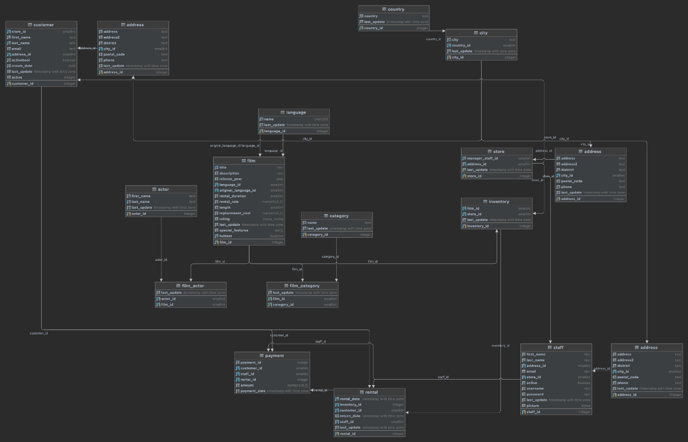
Pattern 3: Multiple Databases
Similar to how individual schemas allow us to organize tables and other database objects and provide better separation of concerns, we can use databases the same way. For example, we could choose to spread the Pagila data across more than one database within a single RDS database instance. Again, using DDD concepts, while schemas might represent Bounded Contexts, databases most closely align to Domains, which are “spheres of knowledge and activity where the application logic revolves” (hackernoon.com).

With Pattern 3, as an organization continues to refine its microservices-based application architecture, it might find that multiple databases within the same database instance are advantageous to further separate and organize application data.

Let’s assume that the data in the films schema is owned and managed by a completely separate team who should never have access to sensitive data stored in the customers, stores, and sales schemas. According to the PostgreSQL docs, database access permissions are managed using the concept of roles. Depending on how the role is set up, a role can be thought of as either a database user or a group of users.
To provide greater separation of concerns than just schemas, we can create a second, completely separate database within the same RDS database instance for data related to films. With two separate databases, it is easier to create and manage distinct roles and ensure access to customers, stores, or sales data is only accessible to teams that need access.
Below, we see the new layout of tables now spread across two databases within the same RDS database instance. Two new tables, highlighted in bold, are explained below.
-----------+----------+-----------+---------------
 Instance  | Database | Schema    | Table
-----------+----------+-----------+---------------
 postgres1 | pagila   | common    | city
 postgres1 | pagila   | common    | country
-----------+----------+-----------+---------------
 postgres1 | pagila   | customers | address
 postgres1 | pagila   | customers | customer
-----------+----------+-----------+---------------
 postgres1 | pagila   | films     | film
-----------+----------+-----------+---------------
 postgres1 | pagila   | sales     | payment
 postgres1 | pagila   | sales     | rental
-----------+----------+-----------+---------------
 postgres1 | pagila   | staff     | address
 postgres1 | pagila   | staff     | staff
-----------+----------+-----------+---------------
 postgres1 | pagila   | stores    | address
 postgres1 | pagila   | stores    | inventory
 postgres1 | pagila   | stores    | store
-----------+----------+-----------+---------------
 postgres1 | products | films     | actor
 postgres1 | products | films     | category
 postgres1 | products | films     | film
 postgres1 | products | films     | film_actor
 postgres1 | products | films     | film_category
 postgres1 | products | films     | language
 postgres1 | products | films     | outbox
Change Data Capture and the Outbox Pattern
Inserts, updates, and deletes of film data can be replicated between the two databases using several methods, including Change Data Capture (CDC) with the Outbox Pattern. CDC is “a pattern that enables database changes to be monitored and propagated to downstream systems” (RedHat). The Outbox Pattern uses the PostgreSQL database’s ability to perform an commit to two tables atomically using a transaction. Transactions bundles multiple steps into a single, all-or-nothing operation.
In this example, data is written to existing tables in the products.films schema (updated aggregate’s state) as well as a new products.films.outbox table (new domain events), wrapped in a transaction. Using CDC, the domain events from the products.films.outbox table are replicated to the pagila.films.film table. The replication of data between the two databases using CDC is also referred to as eventual consistency.

In this example, films in the pagila.films.film and products.films.outbox tables are represented in a denormalized, aggregated view of a film instead of the original, normalized relational multi-table structure. The table definition of the new pagila.films.film table is very different than that of the original Pagila products.films.films table. A concept such as a film, represented as an aggregate or entity, can be common to multiple Bounded Contexts, yet have a different definition.
Note the Confluent JDBC Source Connector (io.confluent.connect.jdbc.JdbcSourceConnector) used here will not work with PostgreSQL arrays, which would be ideal for one-to-many categories and actors columns. Arrays can be converted to text using ::text or by building value-delimited strings using string_agg aggregate function.
Given this table definition, the resulting data would look as follows.
The existing pagila.stores.inventory table has a foreign key constraint on the the pagila.films.film table. However, the films schema and associated tables have been migrated to the products database’s films schema. To overcome this challenge, we can:
- Create a new
pagila.films.filmtable - Continuously replicate data from the
productsdatabase to thepagila.films.filmtable data using CDC (see below) - Modify the
pagila.stores.inventorytable to take a dependency on the newfilmtable - Drop the duplicate tables and other objects from the
pagila.filmsschema
Debezium and Confluent for CDC
There are several technology choices for performing CDC. For this post, I have used RedHat’s Debezium connector for PostgreSQL and Debezium Outbox Event Router, and Confluent’s JDBC Sink Connector. Below, we see a typical example of a Kafka Connect Source Connector using the Debezium connector for PostgreSQL and a Sink Connector using the Confluent JDBC Sink Connector. The Source Connector streams changes from the products logs, using PostgreSQL’s Write-Ahead Logging (WAL) feature, to an Apache Kafka topic. A corresponding Sink Connector streams the changes from the Kafka topic to the pagila database.
Pattern 4: Multiple Database Instances
At some point in the evolution of a microservices-based application, it might become advantageous to separate the data into multiple database instances using the same database engine. Although managing numerous database instances may require more resources, there are also advantages. Each database instance will have independent connection configurations, roles, and administrators. Each database instance could run different versions of the database engine, and each could be upgraded and maintained independently.

With Pattern 4, as an organization continues to refine its application architecture, it might find that multiple database instances are beneficial to further separate and organize application data.

Below is one possible refactoring of the Pagila database, splitting the data between two database engines. The first database instance, postgres1, contains two databases, pagila and products. The second database instance, postgres2, contains a single database, products.
-----------+----------+-----------+---------------
 Instance  | Database | Schema    | Table
-----------+----------+-----------+---------------
 postgres1 | pagila   | common    | city
 postgres1 | pagila   | common    | country
-----------+----------+-----------+---------------
 postgres1 | pagila   | customers | address
 postgres1 | pagila   | customers | customer
-----------+----------+-----------+---------------
 postgres1 | pagila   | films     | actor
 postgres1 | pagila   | films     | category
 postgres1 | pagila   | films     | film
 postgres1 | pagila   | films     | film_actor
 postgres1 | pagila   | films     | film_category
 postgres1 | pagila   | films     | language
-----------+----------+-----------+---------------
 postgres1 | pagila   | staff     | address
 postgres1 | pagila   | staff     | staff
-----------+----------+-----------+---------------
 postgres1 | pagila   | stores    | address
 postgres1 | pagila   | stores    | inventory
 postgres1 | pagila   | stores    | store
-----------+----------+-----------+---------------
 postgres1 | pagila   | sales     | payment
 postgres1 | pagila   | sales     | rental
-----------+----------+-----------+---------------
 postgres2 | products | films     | actor
 postgres2 | products | films     | category
 postgres2 | products | films     | film
 postgres2 | products | films     | film_actor
 postgres2 | products | films     | film_category
 postgres2 | products | films     | language
Data Replication with CDC
Note the films schema is duplicated between the two databases, shown above. Again, using the CDC allows us to keep the six postgres1.pagila.films tables in sync with the six postgres2.products.films tables using CDC. In this example, we are not using the OutBox Pattern, as used previously in Pattern 3. Instead, we are replicating any changes to any of the tables in postgres2.products.films schema to the corresponding tables in the postgres1.pagila.films schema.

To ensure the tables stay in sync, the tables and other objects in the postgres1.pagila.films schema should be limited to read-only access (SELECT) for all users. The postgres2.products.films tables represent the authoritative source of data, the System of Record (SoR). Any inserts, updates, or deletes, must be made to these tables and replicated using CDC.
Pattern 5: Multiple Database Engines
AWS commonly uses the term ‘purpose-built databases.’ AWS offers over fifteen purpose-built database engines to support diverse data models, including relational, key-value, document, in-memory, graph, time series, wide column, and ledger. There may be instances where using multiple, purpose-built databases makes sense. Using different database engines allows architects to take advantage of the unique characteristics of each engine type to support diverse application requirements.
With Pattern 5, as an organization continues to refine its application architecture, it might choose to leverage multiple, different database engines.

Take for example an application that uses a combination of relational, NoSQL, and in-memory databases to persist data. In addition to PostgreSQL, the application benefits from moving a certain subset of its relational data to a non-relational, high-performance key-value store, such as Amazon DynamoDB. Furthermore, the application implements a database cache using an ultra-fast in-memory database, such as Amazon ElastiCache for Redis.
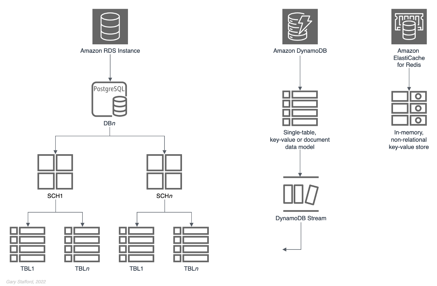
Below is one possible refactoring of the Pagila database, splitting the data between two different database engines, PostgreSQL and Amazon DynamoDB.
-----------+----------+-----------+-----------
 Instance  | Database | Schema    | Table
-----------+----------+-----------+-----------
 postgres1 | pagila   | common    | city
 postgres1 | pagila   | common    | country
-----------+----------+-----------+-----------
 postgres1 | pagila   | customers | address
 postgres1 | pagila   | customers | customer
-----------+----------+-----------+-----------
 postgres1 | pagila   | films     | film
-----------+----------+-----------+-----------
 postgres1 | sales    | sales     | payment
 postgres1 | sales    | sales     | rental
-----------+----------+-----------+-----------
 postgres1 | pagila   | staff     | address
 postgres1 | pagila   | staff     | staff
-----------+----------+-----------+-----------
 postgres1 | pagila   | stores    | address
 postgres1 | pagila   | stores    | film
 postgres1 | pagila   | stores    | inventory
 postgres1 | pagila   | stores    | store
-----------+----------+-----------+-----------
 DynamoDB  |    -     |     -     | Films
The assumption is that based on the application’s access patterns for film data, the application could benefit from the addition of a non-relational, high-performance key-value store. Further, the film-related data entities, such as a film , category, and actor, could be modeled using DynamoDB’s single-table data model architecture. In this model, multiple entity types can be stored in the same table. If necessary, to replicate data back to the PostgreSQL instance from the DynamoBD instance, we can perform CDC with DynamoDB Streams.

Films data model for DynamoDB using NoSQL Workbench
Films data modelCQRS
Command Query Responsibility Segregation (CQRS), a popular software architectural pattern, is another use case for multiple database engines. The CQRS pattern is, as the name implies, “a software design pattern that separates command activities from query activities. In CQRS parlance, a command writes data to a data source. A query reads data from a data source. CQRS addresses the problem of data access performance degradation when applications running at web-scale have too much burden placed on the physical database and the network on which it resides” (RedHat). CQRS commonly uses one database engine optimized for writes and a separate database optimized for reads.

Conclusion
Embracing a microservices-based application architecture may have many business advantages for an organization. However, ignoring the application’s existing databases can negate many of the benefits of microservices. This post examined several common patterns for refactoring relational databases to match a modern microservices-based application architecture.
This blog represents my own viewpoints and not of my employer, Amazon Web Services (AWS). All product names, logos, and brands are the property of their respective owners. All diagrams and illustrations are property of the author.
End-to-End Data Discovery, Observability, and Governance on AWS with LinkedIn’s Open-source DataHub
Posted by Gary A. Stafford in Analytics, AWS, Azure, Bash Scripting, Build Automation, Cloud, DevOps, GCP, Kubernetes, Python, Software Development, SQL, Technology Consulting on March 26, 2022
Use DataHub’s data catalog capabilities to collect, organize, enrich, and search for metadata across multiple platforms
Introduction
According to Shirshanka Das, Founder of LinkedIn DataHub, Apache Gobblin, and Acryl Data, one of the simplest definitions for a data catalog can be found on the Oracle website: “Simply put, a data catalog is an organized inventory of data assets in the organization. It uses metadata to help organizations manage their data. It also helps data professionals collect, organize, access, and enrich metadata to support data discovery and governance.”
Another succinct description of a data catalog’s purpose comes from Alation: “a collection of metadata, combined with data management and search tools, that helps analysts and other data users to find the data that they need, serves as an inventory of available data, and provides information to evaluate the fitness of data for intended uses.”
Working with many organizations in the area of Analytics, one of the more common requests I receive regards choosing and implementing a data catalog. Organizations have datasources hosted in corporate data centers, on AWS, by SaaS providers, and with other Cloud Service Providers. Several of these organizations have recently gravitated to DataHub, the open-source metadata platform for the modern data stack, originally developed by LinkedIn.

In this post, we will explore the capabilities of DataHub to build a centralized data catalog on AWS for datasources hosted in multiple AWS accounts, SaaS providers, cloud service providers, and corporate data centers. I will demonstrate how to build a DataHub data catalog using out-of-the-box data source plugins for automated metadata ingestion.
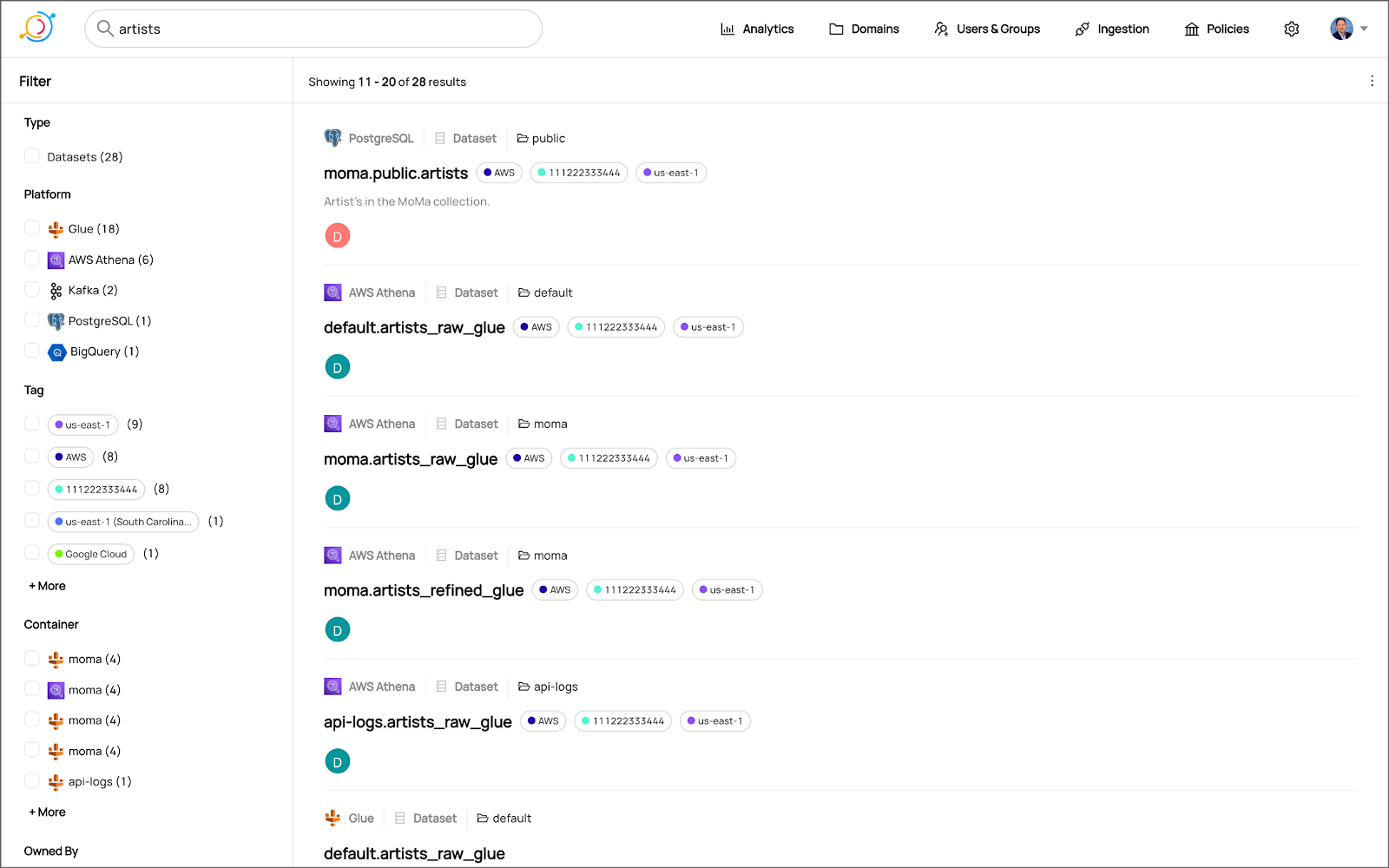
Data Catalog Competitors
Data catalogs are not new; technologies such as data dictionaries have been around as far back as the 1980’s. Gartner publishes their Metadata Management (EMM) Solutions Reviews and Ratings and Metadata Management Magic Quadrant. These reports contain a comprehensive list of traditional commercial enterprise players, modern cloud-native SaaS vendors, and Cloud Service Provider (CSP) offerings. DBMS Tools also hosts a comprehensive list of 30 data catalogs. A sampling of current data catalogs includes:
Open Source Software
Commercial
- Acryl Data (based on LinkedIn’s DataHub)
- Atlan
- Stemma (based on Lyft’s Amundsen)
- Talend
- Alation
- Collibra
- data.world
Cloud Service Providers
Data Catalog Features
DataHub describes itself as “a modern data catalog built to enable end-to-end data discovery, data observability, and data governance.” Sorting through vendor’s marketing jargon and hype, standard features of leading data catalogs include:
- Metadata ingestion
- Data discovery
- Data governance
- Data observability
- Data lineage
- Data dictionary
- Data classification
- Usage/popularity statistics
- Sensitive data handling
- Data fitness (aka data quality or data profiling)
- Manage both technical and business metadata
- Business glossary
- Tagging
- Natively supported datasource integrations
- Advanced metadata search
- Fine-grain authentication and authorization
- UI- and API-based interaction
Datasources
When considering a data catalog solution, in my experience, the most common datasources that customers want to discover, inventory, and search include:
- Relational databases and other OLTP datasources such as PostgreSQL, MySQL, Microsoft SQL Server, and Oracle
- Cloud Data Warehouses and other OLAP datasources such as Amazon Redshift, Snowflake, and Google BigQuery
- NoSQL datasources such as MongoDB, MongoDB Atlas, and Azure Cosmos DB
- Persistent event-streaming platforms such as Apache Kafka (Amazon MSK and Confluent)
- Distributed storage datasets (e.g., Data Lakes) such as Amazon S3, Apache Hive, and AWS Glue Data Catalogs
- Business Intelligence (BI), dashboards, and data visualization sources such as Looker, Tableau, and Microsoft Power BI
- ETL sources, such as Apache Spark, Apache Airflow, Apache NiFi, and dbt
DataHub on AWS
DataHub’s convenient AWS setup guide covers options to deploy DataHub to AWS. For this post, I have hosted DataHub on Kubernetes, using Amazon Elastic Kubernetes Service (Amazon EKS). Alternately, you could choose Google Kubernetes Engine (GKE) on Google Cloud or Azure Kubernetes Service (AKS) on Microsoft Azure.
Conveniently, DataHub offers a Helm chart, making deployment to Kubernetes straightforward. Furthermore, Helm charts are easily integrated with popular CI/CD tools. For this post, I’ve used ArgoCD, the declarative GitOps continuous delivery tool for Kubernetes, to deploy the DataHub Helm charts to Amazon EKS.

According to the documentation, DataHub consists of four main components: GMS, MAE Consumer (optional), MCE Consumer (optional), and Frontend. Kubernetes deployment for each of the components is defined as sub-charts under the main DataHub Helm chart.
External Storage Layer Dependencies
Four external storage layer dependencies power the main DataHub components: Kafka, Local DB (MySQL, Postgres, or MariaDB), Search Index (Elasticsearch), and Graph Index (Neo4j or Elasticsearch). DataHub has provided a separate DataHub Prerequisites Helm chart for the dependencies. The dependencies must be deployed before deploying DataHub.
Alternately, you can substitute AWS managed services for the external storage layer dependencies, which is also detailed in the Deploying to AWS documentation. AWS managed service dependency substitutions include Amazon RDS for MySQL, Amazon OpenSearch (fka Amazon Elasticsearch), and Amazon Managed Streaming for Apache Kafka (Amazon MSK). According to DataHub, support for using AWS Neptune as the Graph Index is coming soon.
DataHub CLI and Plug-ins
DataHub comes with the datahub CLI, allowing you to perform many common operations on the command line. You can install and use the DataHub CLI within your development environment or integrate it with your CI/CD tooling.

DataHub uses a plugin architecture. Plugins allow you to install only the datasource dependencies you need. For example, if you want to ingest metadata from Amazon Athena, just install the Athena plugin: pip install 'acryl-datahub[athena]'. DataHub Source, Sink, and Transformer plugins can be displayed using the datahub check plugins CLI command.


Secure Metadata Ingestion
Often, datasources are not externally accessible for security reasons. Further, many datasources may not be accessible to individual users, especially in higher environments like UAT, Staging, and Production. They are only accessible to applications or CI/CD tooling. To overcome these limitations when extracting metadata with DataHub, I prefer to perform my DataHub-related development and testing locally but execute all DataHub ingestion securely on AWS.
In my local development environment, I use JetBrains PyCharm to author the Python and YAML-based DataHub configuration files and ingestion pipeline recipes, then commit those files to git and push them to a private GitHub repository. Finally, I use GitHub Actions to test DataHub files.
To run DataHub ingestion jobs and push the results to DataHub running in Kubernetes on Amazon EKS, I have built a custom Python-based Docker container. The container runs the DataHub CLI, required DataHub plugins, and any additional Python dependencies. The container’s pod has the appropriate AWS IAM permissions, using IAM Roles for Service Accounts (IRSA), to securely access datasources to ingest and the DataHub application.
Schedule and Monitor Pipelines
Scheduling and managing multiple metadata ingestion jobs on AWS is best handled with Apache Airflow with Amazon Managed Workflows for Apache Airflow (Amazon MWAA). Ingestion jobs run as Airflow DAG tasks, which call the EKS-based DataHub CLI container. With MWAA, datasource connections, credentials, and other sensitive configurations can be kept secure and not be exposed externally or in plain text.
When running the ingestion pipelines on AWS with DataHub, all communications between AWS-based datasources, ingestion jobs running in Airflow, and DataHub, should use secure private IP addressing and DNS resolution instead of transferring metadata over the Internet. Make sure to create all the necessary VPC peering connections, network route table configurations, and VPC endpoints to connect all relevant services.
SaaS services such as Snowflake or MongoDB Atlas, services provided by other Cloud Service Providers such as Google Cloud and Microsoft Azure, and datasources in corporate datasources require alternate networking and security strategies to access metadata securely.

Markup or Code?
According to the documentation, a DataHub recipe is a configuration file that tells ingestion scripts where to pull data from (source) and where to put it (sink). Recipes normally contain a source, sink, and transformers configuration section. Mark-up language-based job automation written in YAML, JSON, or Domain Specific Languages (DSLs) is often an alternative to writing code. DataHub recipes can be written in YAML. The example recipe shown below is used to ingest metadata from an Amazon RDS for PostgreSQL database, running on AWS.
YAML-based recipes can also use automatic environment variable expansion for convenience, automation, and security. It is considered best practice to secure sensitive configuration values, such as database credentials, in a secure location and reference them as environment variables. For example, note the server: ${DATAHUB_REST_ENDPOINT} entry in the sink section below. The DATAHUB_REST_ENDPOINT environment variable is set ahead of time and re-used for all ingestion jobs. Sensitive database connection information has also been variablized and stored separately.
Using Python
You can configure and run a pipeline entirely from within a custom Python script using DataHub’s Python API as an alternative to YAML. Below, we see two nearly identical ingestion recipes to the YAML above, written in Python. Writing ingestion pipeline logic programmatically gives you increased flexibility for automation, error checking, unit-testing, and notification. Below is a basic pipeline written in Python. The code is functional, but not very Pythonic, secure, scalable, or Production ready.
The second version of the same pipeline is more Production ready. The code is more Pythonic in nature and makes use of error checking, logging, and the AWS Systems Manager (SSM) Parameter Store. Like recipes written in YAML, environment variables can be used for convenience and security. In this example, commonly reused and sensitive connection configuration items have been extracted and placed in the SSM Parameter Store. Additional configuration is pulled from the environment, such as AWS Account ID and AWS Region. The script loads these values at runtime.
Sinking to DataHub
When syncing metadata to DataHub, you have two choices, the GMS REST API or Kafka. According to DataHub, the advantage of the REST-based interface is that any errors can immediately be reported. On the other hand, the advantage of the Kafka-based interface is that it is asynchronous and can handle higher throughput. For this post, I am DataHub’s REST API.


Column-level Metadata
In addition to column names and data types, it is possible to extract column descriptions and key types from certain datasources. Column descriptions, tags, and glossary terms can also be input through the DataHub UI. Below, we see an example of an Amazon Redshift fact table, whose table and column descriptions were ingested as part of the metadata.

Business Glossary
DataHub can assign business glossary terms to entities. The DataHub Business Glossary plugin pulls business glossary metadata from a YAML-based configuration file.
Business glossary terms can be reviewed in the Glossary Terms tab of the DataHub’s UI. Below, we see the three terms associated with the Classification glossary node: Confidential, HighlyConfidential, and Sensitive.

We can search for entities inventoried in DataHub using their assigned business glossary terms.

Finally, we see an example of an AWS Athena data catalog table with business glossary terms applied to columns within the table’s schema.

SQL-based Profiler
DataHub also can extract statistics about entities in DataHub using the SQL-based Profiler. According to the DataHub documentation, the Profiler can extract the following:
- Row and column counts for each table
- Column null counts and proportions
- Column distinct counts and proportions
- Column min, max, mean, median, standard deviation, quantile values
- Column histograms or frequencies of unique values
In addition, we can also track the historical stats for each profiled entity each time metadata is ingested.


Data Lineage
DataHub’s data lineage features allow us to view upstream and downstream relationships between different types of entities. DataHub can trace lineage across multiple platforms, datasets, pipelines, charts, and dashboards.
Below, we see a simple example of dataset entity-to-entity lineage in Amazon Redshift and then Apache Spark on Amazon EMR. The fact table has a downstream relationship to four database views. The views are based on SQL queries that include the upstream table as a datasource.


DataHub Analytics
DataHub provides basic metadata quality and usage analytics in the DataHub UI: user activity, counts of datasource types, business glossary terms, environments, and actions.


Conclusion
In this post, we explored the features of a data catalog and learned about some of the leading commercial and open-source data catalogs. Next, we learned how DataHub could collect, organize, enrich, and search metadata across multiple datasources. Lastly, we discovered how easy it is to catalog metadata from datasources spread across multiple CSP, SaaS providers, and corporate data centers, and centralize those results in DataHub.
In addition to the basic features reviewed in this post, DataHub offers a growing number of additional capabilities, including GraphQL and Timeline APIs, robust authentication and authorization, application monitoring observability, and Great Expectations integration. All these qualities make DataHub an excellent choice for a data catalog.
This blog represents my own viewpoints and not of my employer, Amazon Web Services (AWS). All product names, logos, and brands are the property of their respective owners.
Data Preparation on AWS: Comparing Available ELT Options to Cleanse and Normalize Data
Posted by Gary A. Stafford in Analytics, AWS, Build Automation, Cloud, Python, SQL, Technology Consulting on March 1, 2022
Comparing the features and performance of different AWS analytics services for Extract, Load, Transform (ELT)
Introduction
According to Wikipedia, “Extract, load, transform (ELT) is an alternative to extract, transform, load (ETL) used with data lake implementations. In contrast to ETL, in ELT models the data is not transformed on entry to the data lake but stored in its original raw format. This enables faster loading times. However, ELT requires sufficient processing power within the data processing engine to carry out the transformation on demand, to return the results in a timely manner.”
As capital investments and customer demand continue to drive the growth of the cloud-based analytics market, the choice of tools seems endless, and that can be a problem. Customers face a constant barrage of commercial and open-source tools for their batch, streaming, and interactive exploratory data analytics needs. The major Cloud Service Providers (CSPs) have even grown to a point where they now offer multiple services to accomplish similar analytics tasks.
This post will examine the choice of analytics services available on AWS capable of performing ELT. Specifically, this post will compare the features and performance of AWS Glue Studio, Amazon Glue DataBrew, Amazon Athena, and Amazon EMR using multiple ELT use cases and service configurations.
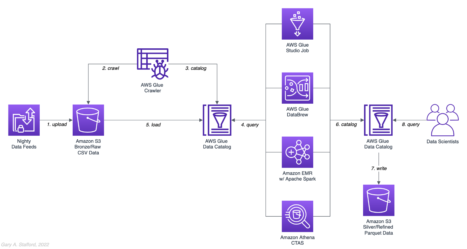
Analytics Use Case
We will address a simple yet common analytics challenge for this comparison — preparing a nightly data feed for analysis the next day. Each night a batch of approximately 1.2 GB of raw CSV-format healthcare data will be exported from a Patient Administration System (PAS) and uploaded to Amazon S3. The data must be cleansed, deduplicated, refined, normalized, and made available to the Data Science team the following morning. The team of Data Scientists will perform complex data analytics on the data and build machine learning models designed for early disease detection and prevention.
Sample Dataset
The dataset used for this comparison is generated by Synthea, an open-source patient population simulation. The high-quality, synthetic, realistic patient data and associated health records cover every aspect of healthcare. The dataset contains the patient-related healthcare history for allergies, care plans, conditions, devices, encounters, imaging studies, immunizations, medications, observations, organizations, patients, payers, procedures, providers, and supplies.
The Synthea dataset was first introduced in my March 2021 post examining the handling of sensitive PII data using Amazon Macie: Data Lakes: Discovery, Security, and Privacy of Sensitive Data.
The Synthea synthetic patient data is available in different record volumes and various data formats, including HL7 FHIR, C-CDA, and CSV. We will use CSV-format data files for this post. Since this post seeks to measure the performance of different AWS ELT-capable services, we will use a larger version of the Synthea dataset containing hundreds of thousands to millions of records.
AWS Glue Data Catalog
The dataset comprises nine uncompressed CSV files uploaded to Amazon S3 and cataloged to an AWS Glue Data Catalog, a persistent metadata store, using an AWS Glue Crawler.

Test Cases
We will use three data preparation test cases based on the Synthea dataset to examine the different AWS ELT-capable services.

Test Case 1: Encounters for Symptom
An encounter is a health care contact between the patient and the provider responsible for diagnosing and treating the patient. In our first test case, we will process 1.26M encounters records for an ongoing study of patient symptoms by our Data Science team.
Data preparation includes the following steps:
- Load 1.26M encounter records using the existing AWS Glue Data Catalog table.
- Remove any duplicate records.
- Select only the records where the
descriptioncolumn contains “Encounter for symptom.” - Remove any rows with an empty
reasoncodescolumn. - Extract a new
year,month, anddaycolumn from thedatecolumn. - Remove the
datecolumn. - Write resulting dataset back to Amazon S3 as Snappy-compressed Apache Parquet files, partitioned by
year,month, andday. - Given the small resultset, bucket the data such that only one file is written per
daypartition to minimize the impact of too many small files on future query performance. - Catalog resulting dataset to a new table in the existing AWS Glue Data Catalog, including partitions.
Test Case 2: Observations
Clinical observations ensure that treatment plans are up-to-date and correctly administered and allow healthcare staff to carry out timely and regular bedside assessments. We will process 5.38M encounters records for our Data Science team in our second test case.
Data preparation includes the following steps:
- Load 5.38M observation records using the existing AWS Glue Data Catalog table.
- Remove any duplicate records.
- Extract a new
year,month, anddaycolumn from the date column. - Remove the
datecolumn. - Write resulting dataset back to Amazon S3 as Snappy-compressed Apache Parquet files, partitioned by
year,month, andday. - Given the small resultset, bucket the data such that only one file is written per
daypartition to minimize the impact of too many small files on future query performance. - Catalog resulting dataset to a new table in the existing AWS Glue Data Catalog, including partitions.
Test Case 3: Sinusitis Study
A medical condition is a broad term that includes all diseases, lesions, and disorders. In our second test case, we will join the conditions records with the patient records and filter for any condition containing the term ‘sinusitis’ in preparation for our Data Science team.
Data preparation includes the following steps:
- Load 483k condition records using the existing AWS Glue Data Catalog table.
- Inner join the condition records with the 132k patient records based on patient ID.
- Remove any duplicate records.
- Drop approximately 15 unneeded columns.
- Select only the records where the
descriptioncolumn contains the term “sinusitis.” - Remove any rows with empty
ethnicity,race,gender, ormaritalcolumns. - Create a new column,
condition_age, based on a calculation of the age in days at which the patient’s condition was diagnosed. - Write the resulting dataset back to Amazon S3 as Snappy-compressed Apache Parquet-format files. No partitions are necessary.
- Given the small resultset, bucket the data such that only one file is written to minimize the impact of too many small files on future query performance.
- Catalog resulting dataset to a new table in the existing AWS Glue Data Catalog.
AWS ELT Options
There are numerous options on AWS to handle the batch transformation use case described above; a non-exhaustive list includes:
- AWS Glue Studio (UI-driven with AWS Glue PySpark Extensions)
- Amazon Glue DataBrew
- Amazon Athena
- Amazon EMR with Apache Spark
- AWS Glue Studio (Apache Spark script)
- AWS Glue Jobs (Legacy jobs)
- Amazon EMR with Presto
- Amazon EMR with Trino
- Amazon EMR with Hive
- AWS Step Functions and AWS Lambda
- Amazon Redshift Spectrum
- Partner solutions on AWS, such as Databricks, Snowflake, Upsolver, StreamSets, Stitch, and Fivetran
- Self-managed custom solutions using a combination of OSS, such as dbt, Airbyte, Dagster, Meltano, Apache NiFi, Apache Drill, Apache Beam, Pandas, Apache Airflow, and Kubernetes
For this comparison, we will choose the first five options listed above to develop our ELT data preparation pipelines: AWS Glue Studio (UI-driven job creation with AWS Glue PySpark Extensions), Amazon Glue DataBrew, Amazon Athena, Amazon EMR with Apache Spark, and AWS Glue Studio (Apache Spark script).
AWS Glue Studio
According to the documentation, “AWS Glue Studio is a new graphical interface that makes it easy to create, run, and monitor extract, transform, and load (ETL) jobs in AWS Glue. You can visually compose data transformation workflows and seamlessly run them on AWS Glue’s Apache Spark-based serverless ETL engine. You can inspect the schema and data results in each step of the job.”
AWS Glue Studio’s visual job creation capability uses the AWS Glue PySpark Extensions, an extension of the PySpark Python dialect for scripting ETL jobs. The extensions provide easier integration with AWS Glue Data Catalog and other AWS-managed data services. As opposed to using the graphical interface for creating jobs with AWS Glue PySpark Extensions, you can also run your Spark scripts with AWS Glue Studio. In fact, we can use the exact same scripts run on Amazon EMR.
For the tests, we are using the G.2X worker type, Glue version 3.0 (Spark 3.1.1 and Python 3.7), and Python as the language choice for this comparison. We will test three worker configurations using both UI-driven job creation with AWS Glue PySpark Extensions and Apache Spark script options:
- 10 workers with a maximum of 20 DPUs
- 20 workers with a maximum of 40 DPUs
- 40 workers with a maximum of 80 DPUs


AWS Glue DataBrew
According to the documentation, “AWS Glue DataBrew is a visual data preparation tool that enables users to clean and normalize data without writing any code. Using DataBrew helps reduce the time it takes to prepare data for analytics and machine learning (ML) by up to 80 percent, compared to custom-developed data preparation. You can choose from over 250 ready-made transformations to automate data preparation tasks, such as filtering anomalies, converting data to standard formats, and correcting invalid values.”
DataBrew allows you to set the maximum number of DataBrew nodes that can be allocated when a job runs. For this comparison, we will test three different node configurations:
- 3 maximum nodes
- 10 maximum nodes
- 20 maximum nodes


Amazon Athena
According to the documentation, “Athena helps you analyze unstructured, semi-structured, and structured data stored in Amazon S3. Examples include CSV, JSON, or columnar data formats such as Apache Parquet and Apache ORC. You can use Athena to run ad-hoc queries using ANSI SQL, without the need to aggregate or load the data into Athena.”
Although Athena is classified as an ad-hoc query engine, using a CREATE TABLE AS SELECT (CTAS) query, we can create a new table in the AWS Glue Data Catalog and write to Amazon S3 from the results of a SELECT statement from another query. That other query statement performs a transformation on the data using SQL.
Amazon Athena is a fully managed AWS service and has no performance settings to adjust or monitor.


CTAS and Partitions
A notable limitation of Amazon Athena for the batch use case is the 100 partition limit with CTAS queries. Athena [only] supports writing to 100 unique partition and bucket combinations with CTAS. Partitioned by year, month, and day, the observations test case requires 2,558 partitions, and the observations test case requires 10,433 partitions. There is a recommended workaround using an INSERT INTO statement. However, the workaround requires additional SQL logic, computation, and most important cost. It is not practical, in my opinion, compared to other methods when a higher number of partitions are needed. To avoid the partition limit with CTAS, we will only partition by year and bucket by month when using Athena. Take this limitation into account when comparing the final results.
Amazon EMR with Apache Spark
According to the documentation, “Amazon EMR is a cloud big data platform for running large-scale distributed data processing jobs, interactive SQL queries, and machine learning (ML) applications using open-source analytics frameworks such as Apache Spark, Apache Hive, and Presto. You can quickly and easily create managed Spark clusters from the AWS Management Console, AWS CLI, or the Amazon EMR API.”
For this comparison, we are using two different Spark 3.1.2 EMR clusters:
- (1) r5.xlarge Master node and (2) r5.2xlarge Core nodes
- (1) r5.2xlarge Master node and (4) r5.2xlarge Core nodes
All Spark jobs are written in both Python (PySpark) and Scala. We are using the AWS Glue Data Catalog as the metastore for Spark SQL instead of Apache Hive.


Results
Data pipelines were developed and tested for each of the three test cases using the five chosen AWS ELT services and configuration variations. Each pipeline was then run 3–5 times, for a total of approximately 150 runs. The resulting AWS Glue Data Catalog table and data in Amazon S3 were deleted between each pipeline run. Each new run created a new data catalog table and wrote new results to Amazon S3. The median execution times from these tests are shown below.


Although we can make some general observations about the execution times of the chosen AWS services, the results are not meant to be a definitive guide to performance. An accurate comparison would require a deeper understanding of how each of these managed services works under the hood, in order to both optimize and balance their compute profiles correctly.
Amazon Athena
The Resultset column contains the final number of records written to Amazon S3 by Athena. The results contain the data pipeline’s median execution time and any additional data points.

AWS Glue Studio (AWS Glue PySpark Extensions)
Tests were run with three different configurations for AWS Glue Studio using the graphical interface for creating jobs with AWS Glue PySpark Extensions. Times for each configuration were nearly identical.

AWS Glue Studio (Apache PySpark script)
As opposed to using the graphical interface for creating jobs with AWS Glue PySpark Extensions, you can also run your Apache Spark scripts with AWS Glue Studio. The tests were run with the same three configurations as above. The execution times compared to the Amazon EMR tests, below, are almost identical.

Amazon EMR with Apache Spark
Tests were run with three different configurations for Amazon EMR with Apache Spark using PySpark. The first set of results is for the 2-node EMR cluster. The second set of results is for the 4-node cluster. The third set of results is for the same 4-node cluster in which the data was not bucketed into a single file within each partition. Compare the execution times and the number of objects against the previous set of results. Too many small files can negatively impact query performance.

It is commonly stated that “Scala is almost ten times faster than Python.” However, with Amazon EMR, jobs written in Python (PySpark) and Scala had similar execution times for all three test cases.

Amazon Glue DataBrew
Tests were run with three different configurations Amazon Glue DataBrew, including 3, 10, and 20 maximum nodes. Times for each configuration were nearly identical.

Observations
- All tested AWS services can read and write to an AWS Glue Data Catalog and the underlying datastore, Amazon S3. In addition, they all work with the most common analytics data file formats.
- All tested AWS services have rich APIs providing access through the AWS CLI and SDKs, which support multiple programming languages.
- Overall, AWS Glue Studio, using the AWS Glue PySpark Extensions, appears to be the most capable ELT tool of the five services tested and with the best performance.
- Both AWS Glue DataBrew and AWS Glue Studio are no-code or low-code services, democratizing access to data for non-programmers. Conversely, Amazon Athena requires knowledge of ANSI SQL, and Amazon EMR with Apache Spark requires knowledge of Scala or Python. Be cognizant of the potential trade-offs from using no-code or low-code services on observability, configuration control, and automation.
- Both AWS Glue DataBrew and AWS Glue Studio can write a custom Parquet writer type optimized for Dynamic Frames, GlueParquet. One potential advantage, a pre-computed schema is not required before writing.
- There is a slight ‘cold-start’ with Glue Studio. Studio startup times ranged from 7 seconds to 2 minutes and 4 seconds in the tests. However, the lower execution time of AWS Glue Studio compared to Amazon EMR with Spark and AWS Glue DataBrew in the tests offsets any initial cold-start time, in my opinion.
- Changing the maximum number of units from 3 to 10 to 20 for AWS Glue DataBrew made negligible differences in job execution times. Given the nearly identical execution times, it is unclear exactly how many units are being used by the job. More importantly, how many DataBrew node hours we are being billed for. These are some of the trade-offs with a fully-managed service — visibility and fine-tuning configuration.
- Similarly, with AWS Glue Studio, using either 10 workers w/ max. 20 DPUs, 20 workers w/ max. 40 DPUs, or 40 workers w/ max. 80 DPUs resulted in nearly identical executions times.
- Amazon Athena had the fastest execution times but is limited by the 100 partition limit for large CTAS resultsets. Athena is not practical, in my opinion, compared to other ELT methods, when a higher number of partitions are needed.
- It is commonly stated that “Scala is almost ten times faster than Python.” However, with Amazon EMR, jobs written in Python (PySpark) and Scala had almost identical execution times for all three test cases.
- Using Amazon EMR with EC2 instances takes about 9 minutes to provision a new cluster for this comparison fully. Given nearly identical execution times to AWS Glue Studio with Apache Spark scripts, Glue has the clear advantage of nearly instantaneous startup times.
- AWS recently announced Amazon EMR Serverless. Although this service is still in Preview, this new version of EMR could potentially reduce or eliminate the lengthy startup time for ephemeral clusters requirements.
- Although not discussed, scheduling the data pipelines to run each night was a requirement for our use case. AWS Glue Studio jobs and AWS Glue DataBrew jobs are schedulable from those services. For Amazon EMR and Amazon Athena, we could use Amazon Managed Workflows for Apache Airflow (MWAA), AWS Data Pipeline, or AWS Step Functions combined with Amazon CloudWatch Events Rules to schedule the data pipelines.
Conclusion
Customers have many options for ELT — the cleansing, deduplication, refinement, and normalization of raw data. We examined chosen services on AWS, each capable of handling the analytics use case presented. The best choice of tools depends on your specific ELT use case and performance requirements.
This blog represents my own viewpoints and not of my employer, Amazon Web Services (AWS). All product names, logos, and brands are the property of their respective owners.
Considerations for Architecting Resilient Multi-Region Workloads
Posted by Gary A. Stafford in Enterprise Software Development, Technology Consulting on January 24, 2022
What to consider when evaluating a ‘multi-region’ strategy as part of business continuity and disaster recovery planning
Introduction
Increasingly, I hear the term ‘multi-region’ used within the IT community and in conversations with peers and customers, most often within the context of disaster recovery. In my experience, ‘multi-region’ is a cloud provider-agnostic phrase that can mean different things to different organizations. A few examples:
- Multiple, independent, regionally-deployed application instances that better serve a geographically-diverse customer base, for regulated ‘locality-restricted’ workloads, to ensure data sovereignty, distribute system load, or minimize the blast radius of a regional disaster event. Although a disaster recovery plan may be required, the primary driver of this architecture is often not disaster recovery.
- An active-passive failover strategy in which a second DR Region hosts a mixture of cold, warm, and hot copies of workloads and serves as a failover in response to a disaster event in the Primary Region. In my experience, this is probably the most common use case when someone refers to ‘multi-region.’
- An active-active architecture in which data is continually replicated and traffic can be seamlessly routed based on geolocation between all services within two or more geo-redundant regions, making it resilient to the impact of a regional disaster event. Some might describe this architecture as having both inner-regional and inter-regional high availability.

Terminology
The following terminology is commonly used when discussing Business Continuity and Disaster Recovery Planning. Teams should be familiar with these concepts before undertaking planning activities:
- Fault Tolerance (FT), High Availability (HA), Disaster Recovery (DR), and Business Continuity (BC), and the distinct differences between the four concepts
- Business Continuity Plan/Planning (BCP) and Disaster Recovery Plan/Planning (DRP), and the differences between the two types of plans (source)
- Business Continuity and Disaster Recovery (BCDR or BC/DR) (source)
- Business Impact Analysis (BIA) and Risk Assessment (source)
- Categories of Disaster: Natural Disasters, Technical Failures, and Human Actions, both intentional and unintentional (source)
- Resiliency, which includes both Disaster Recovery (service restoration) and Availability (preventing loss of service) (source)
- Crisis Management: Critical vs. Non-Critical Systems and Mission Critical vs. Business Critical Systems (source)
- Regions vs. Availability Zones (aka Zones), common constructs to all major Cloud Service Providers (CSP): AWS, Google Cloud, Microsoft Azure, IBM Cloud, and Oracle Cloud
- Primary (aka Active) Region vs. DR (aka Passive or Standby) Region (source)
- Active-Active vs. Active-Passive DR Strategies (source)
- SHARE’s 7 Tiers of Disaster Recovery (source)
- Disaster Recovery Site Types: Cold, Warm, and Hot (source)
- AWS Multi-Region Disaster Recovery Strategies: 1) Backup and restore, 2) active-passive Pilot light, 3) active-passive Warm standby, or 4) Multi-region (multi-site) active-active (source)
- Recovery Time Objective (RTO) and Recovery Point Objective (RPO), and the methods and costs to achieve varying levels of each SLA (source)
- Failover and Failback Operations (source)
- Partial vs. Complete Regional Outage, and the implications to Disaster Recovery Planning (source)
- Single Points of Failure (SPOF) (source)
BCDR Planning Considerations
When developing BCDR Plans that include multi-region, there are several technical aspects of your workloads that need to be considered. The following list is not designed to be exhaustive, nor is it intended to suggest that multi-region DR is an unattainable task. On the contrary, this list is meant to encourage thorough planning and suggest ways to continually improve an organization’s plan.
- Configuration Data Management
- Secret Management
- Cryptographic Key Management
- Hardware Security Module (HSM)
- Credential Management
- SSL/TLS Certificate Management
- Authentication (AuthN) and Authorization (AuthZ)
- Domain Name System (DNS), DNS Failover and Failback, Global Traffic Management (GTM)
- Content delivery network (CDN)
- Specialized Workloads, such as SAP, VMware, SharePoint, Citrix, Oracle, SQL Server, SAP HANA, and IBM Db2
- On-premises workload dependencies, and wide-area network (WAN) connectivity between on-premises data centers and the Cloud
- Remote access from on-premises and remote employees to cloud-based backend and enterprise systems
- Edge compute, such as connected devices, IoT, storage gateways, and remotely-managed local cloud-infrastructure (e.g., AWS Outposts
- DevOps, CI/CD, Release Management
- Infrastructure as Code (IaC)
- Public and private artifact repositories, including Docker and Virtual Machine (VM) Image repositories
- Source code in Version Control Systems (VCS), also known as Source Control Management (SCM)
- Software licensing for the self-managed and hosted services
- Observability, monitoring, logging, alerting, and notification
- Regional differences of a Cloud Provider’s service offerings, cost, performance, and support
- Latency, including latency between Primary and DR Region and between end-users and partners and DR Region
- Data residency and data sovereignty requirements, which will impact choice of DR Region
- Automated, event-driven Failover process vs. manual processes
- Failback process
- Playbooks, documentation, training, and regular testing
- Support, help desk, and call center coordination (and potential impact of disaster event on Cloud-based call center technologies)
Disaster Recovery Planning Process
In my opinion, many disaster planning discussions I’m involved in begin by focusing on the wrong things. Logically, engineering teams often jump right to questions about specific service capabilities, such as “is my database capable of cross-region replication?” or “how do I support multi-region cryptographic keys for data encryption and decryption.” Yet, higher-level business continuity planning or workload assessments haven’t yet been conducted. Based on my experience, I suggest the following approach to get started with disaster recovery planning (again, not an exhaustive list):
- Workload Portfolio: Identify the organization’s complete workload portfolio, including all distinct applications and their associated infrastructure, datastores, and other dependencies.
- DR Workloads: From the portfolio, identify which workloads are considered business-critical or mission-critical systems and must be part of the disaster recovery planning.
- Classification: Classify each DR workload based on Business Impact Analysis, Risk Assessment, and SLAs such as availability, RTO, and RPO. Do the requirements demand an active-passive or active-active DR strategy? In AWS terms, do the requirements dictate Backup and Restore, Pilot Light, Warm Standby, or Multi-Site Active-Active?
- Documentation: Obtain current documentation and architectural and process-flow diagrams showing all components and dependencies, including cross-workload and third-party dependencies such as SaaS vendors. Review and verify accuracy of documentation and diagrams.
- Current Regions: Identify the Regions into which the existing workload is deployed.
- Service-level Review: Review each workload’s individual components to ensure they can meet the DR requirements, such as compute, storage, databases, security, networking, edge, CDN, mobile, frontend web, and end-user compute (e.g., “is the workload’s specific NoSQL database capable of cross-region replication and automatic failover?”).
- Third-party Dependencies: Identify and review each workload’s third-party dependencies, such as SaaS partners. Is their service essential to a critical workload’s functionality? What is your partner’s Disaster Recovery Plan?
- DR-capable Workload: Determine how much re-engineering is required to deploy and operate the workload to the DR Region.
- Data Residency and Data Sovereignty: Review data residency and sovereignty requirements for the workload, which could impact the choice of DR Regions.
- Choose DR Region: Not all Cloud Provider’s Regions offer the same services. Therefore, choose a DR Region(s) that can support all services utilized by the workload.
- Disaster Planning Considerations: Review all items shown in the previous ‘Disaster Recovery Planning Considerations’ section for each workload.
- Prepare for Partial Failures: Decide how you will handle partial versus complete regional outages. Regional disruptions of specific services are the most common type of Cloud outage, often resulting in partial impairment of a workload.
- Cost: Calculate the cost of the workload based on the required DR Service Level and DR Region. Investigate Cloud-provider’s volume pricing agreements to reduce costs.
- Budget: Adjust DR Service Level requirements to meet budgetary constraints if necessary.
- Re-engineer Workloads: Construct timelines and budgets to re-engineer workloads for DR if required.
- DR Proof of Concept: Build out a Proof of Concept (POC) DR Region to validate the plan’s major assumptions and adjust if necessary; include failover and failback operations.
- DR Buildout: Construct timelines and budgets to build out the DR environment.
- Workload Deployment: Construct timelines and budgets to provision, deploy, configure, test, and monitor workloads in the DR Region.
- Documentation, Training, and Testing: Ensure all playbooks, documentation, training, and testing procedures are completed and regularly reviewed, updated, and tested, including failover and failback operations.
Before Considering Multi-Region
Workloads built to be resilient, fault-tolerant, highly available, easily deployable and configurable, backed-up, and monitored will help an organization withstand the most common disruptions in the Cloud. Before considering a multi-region disaster recovery strategy, I strongly recommend ensuring the following aspects of your workloads are adequately addressed:
- Fault Tolerance: Workloads are architected to be fault-tolerant such that they can withstand the failure of individual components and operate in a degraded state. Eliminate any single point of failure (SPOF).
- High Availability: Workloads are designed to be highly available, which with most cloud providers means resources are spread across multiple, discrete, regionally dispersed data centers or Availability Zones (AZ) and can tolerate the loss of a data center or AZ.
- Backup: All workload components, source code, data, and configuration are regularly backed up using automated processes. All backups are verified. Backups are periodically restored to test restore procedures. As the most basic form of disaster recovery, developing and testing a backup and restore strategy will help teams to think more deeply about disaster planning.
- Observability: Workloads have adequate observability, monitoring, logging, alerting, and notification processes in place.
- Automation: Workloads and all required infrastructure and configuration are codified, documented, and can be efficiently and consistently deployed and configured without requiring manual intervention, using mature DevOps and CI/CD practices. Ensuring workloads can be consistently deployed and re-deployed will help ensure they could be built out in a second region if multi-region is a potential goal.
- Environment-agnostic: Workloads are environment-agnostic, with no hard-coded application or infrastructure dependencies or configurations. Confirming workloads are environment-agnostic will help to ensure they are portable across regions if multi-region is a potential goal.
- Multi-environment: Workloads are deployed to one or more SDLC environments prior to Production, such as Development, Test, Staging, or UAT. The environment should be a different Cloud account than Production. A second environment will help to ensure workloads are portable across regions if multi-region is a potential goal.
- Chaos Engineering: Workloads are regularly tested to ensure that they can withstand unexpected disruptions.
References
In addition to the references already listed, here are some useful references to learn more about the topics introduced in this post:
- AWS: Plan for Disaster Recovery (DR)
- Azure: Backup and disaster recovery
- Google Cloud: Disaster recovery planning guide
- AWS: Disaster Recovery of Workloads on AWS (YouTube video)
- Cloud4U: 7 tiers of disaster recovery
- Barracuda Networks: What is Disaster Recovery?
- Nakivo: An Overview of Disaster Recovery Sites
- NetMotion: Mission Critical Systems vs. Business Critical Systems
- Teceze: Disaster Recovery Plans Vs. Business Continuity Plans
- TechTarget: Chaos Engineering
Conclusion
In this post, we explored some of the potential meanings of the term ‘multi-region’. We then reviewed Business Continuity and Disaster Recovery Planning terminologies, considerations, and a recommended approach to get started. Lastly, we discovered some best-practices to enact before considering a multi-region disaster recovery strategy. What does ‘multi-region’ mean to your organization? Do you have comprehensive Business Continuity and Disaster Recovery Plans for your Cloud-based workloads? I would value your feedback and thoughts.
This blog represents my own viewpoints and not of my employer, Amazon Web Services (AWS). All product names, logos, and brands are the property of their respective owners.
Capturing Data Analytics Workflows and System Requirements
Posted by Gary A. Stafford in Analytics, Big Data, Technology Consulting on January 21, 2022
Implement an effective, consistent, and repeatable strategy for documenting data analytics workflows and capturing system requirements
“Data analytics applications involve more than just analyzing data, particularly on advanced analytics projects. Much of the required work takes place upfront, in collecting, integrating, and preparing data and then developing, testing, and revising analytical models to ensure that they produce accurate results. In addition to data scientists and other data analysts, analytics teams often include data engineers, who create data pipelines and help prepare data sets for analysis.” — TechTarget
Introduction
Successful consultants, project managers, and product owners use well-proven and systematic approaches to achieve desired outcomes, including successful customer engagements, project results, and product and service launches. Modern data stacks and analytics workflows are increasingly complex. This technology-agnostic discovery process aims to help an organization efficiently and repeatably capture a concise record of existing analytics workflows, business and technical goals and constraints, and measures of success. If applicable, the discovery process is also used to compile and clarify requirements for new data analytics workflows.

Analytics Workflow Stages
There are many patterns organizations use to delineate the stages of their analytics workflows. This process utilizes six stages of a typical analytics workflow:
- Generate: All the ways data is generated and the systems of record where it is stored or originates from, also referred to as data ingress
- Collect: All the ways data is collected or ingested
- Prepare: All the ways data is transformed, including ETL, ELT, reverse ETL, and ML
- Store: All the ways data is stored, organized, and secured for analytics purposes
- Analyze: All the ways data is analyzed
- Deliver: All the ways data is delivered and how it is consumed, also referred to as data egress or data products
The precise nomenclature is not critical to this process as long as all major functionality is considered.
The Process
The discovery process starts by working backward. It first identifies existing goals and desired outcomes. It then identifies existing and anticipated future constraints. Next, it breaks down the current analytics workflows, examining the four stages of collect, prepare, store, and analyze, the steps required to get from data sources to deliverables. Finally, it captures the inputs and the outputs for the workflows and the data producers and consumers.
Collect, prepare, store, and analyze — the steps required to get from data sources to deliverables.
Specifically, the process identifies and documents the following:
- Business and technical goals and desired outcomes
- Business and technical constraints also referred to as limitations or restrictions
- Analytics workflows: tools, techniques, procedures, and organizational structure
- Outputs also referred to as deliverables, required to achieve desired outcomes
- Inputs, also referred to as data sources, required to achieve desired outcomes
- Data producers and consumers
- Measures of success
- Recommended next steps
Outcomes
Capture business and technical goals and desired outcomes driving the necessity to rearchitect current analytics processes. For example:
- Re-architect analytics processes to modernize, reduce complexity, or add new capabilities
- Reduce or control costs
- Increase performance, scalability, speed
- Migrate on-premises workloads, workflows, processes to the Cloud
- Migrate from one cloud provider or SaaS provider to another
- Move away from proprietary software products to open source software (OSS) or commercial open source software (COSS)
- Migrate away from custom-built software to commercial off-the-shelf (COTS), OSS, or COSS solutions
- Integrate DevOps, GitOps, DataOps, or MLOps practices
- Integrate on-premises, multi-cloud, and SaaS-based hybrid architectures
- Develop new analytics product or service offerings
- Standardize analytics processes
- Leverage the data for AI and ML purposes
- Provide stakeholders with a real-time business KPIs dashboard
- Construct a data lake, data warehouse, data lakehouse, or data mesh
If migration is involved, review the 6 R’s of Cloud Migration: Rehost, Replatform, Repurchase, Refactor, Retain, or Retire.
Constraints
Identify the existing and potential future business and technical constraints that impact analytics workflows. For example:
- Budgets
- Cost attribution
- Timelines
- Access to skilled resources
- Internal and external regulatory requirements, such as HIPAA, SOC2, FedRAMP, GDPR, PCI DSS, CCPA, and FISMA
- Business Continuity and Disaster Recovery (BCDR) requirements
- Architecture Review Board (ARB), Center of Excellence (CoE), Change Advisory Board (CAB), and Release Management standards and guidelines
- Data residency and data sovereignty requirements
- Security policies
- Service Level Agreements (SLAs); see ‘Measures of Success’ section
- Existing vendor, partner, cloud-provider, and SaaS relationships
- Existing licensing and contractual obligations
- Deprecated code dependencies and other technical debt
- Must-keep aspects of existing processes
- Build versus buy propensity
- Proprietary versus open source software propensity
- Insourcing versus outsourcing propensity
- Managed, hosted, SaaS versus self-managed software propensity

Analytics Workflows
Capture analytics workflows using the four stages of collect, prepare, store, and analyze, as a way to organize the discussion:
- High- and low-level architecture, process flow diagrams, sequence diagrams
- Recent architectural assessments such as reviews based on the AWS Data Analytics Lens, AWS Well-Architected Framework, Microsoft Azure Well-Architected Framework, or Google Cloud Architecture Framework
- Analytics tools, including hardware and commercial, custom, and open-source software
- Security policies, processes, standards, and technologies
- Observability, logging, monitoring, alerting, and notification
- Teams, including roles, responsibilities, and skillsets
- Partners, including consultants, vendors, SaaS providers, and Managed Service Providers (MSP)
- SDLC environments, such as Local, Sandbox, Development, Testing, Staging, Production, and Disaster Recovery (DR)
- Business Continuity Planning (BCP) policies, processes, standards, and technologies
- Primary analytics programming languages
- External system dependencies
- DataOps, MLOps, DevOps, CI/CD, SCM/VCS, and Infrastructure-as-Code (IaC) automation policies, processes, standards, and technologies
- Data governance and data lineage policies, processes, standards, and technologies
- Data quality (or data assurance) policies, processes, standards, technologies, and testing methodologies
- Data anomaly detection policies, processes, standards, and technologies
- Intellectual property (IP), the ‘secret sauce’ that differentiates the organization’s processes and provides a competitive advantage, such as ML models, proprietary algorithms, datasets, highly specialized knowledge, and patents
- Overall effectiveness and customer satisfaction with existing analytics platform (document sources of customer feedback)
- Known deficiencies with current analytics processes

Outputs
Identify the deliverables required to meet the desired outcomes. For example, prepare and provide data for:
- Data analytics purposes
- Business Intelligence (BI), visualizations, and dashboards
- Machine Learning (ML) and Artificial Intelligence (AI)
- Data exports and data feeds, such as Excel or CSV-format files
- Hosted datasets for external or internal consumption
- Data APIs for external or internal consumption
- Documentation, Data API guides, data dictionaries, example code such as Notebooks
- SaaS-based product offering

Inputs
Capture sources of data that are required to produce the outputs. For example:
- Batch sources such as flat files from legacy systems, third-party providers, and enterprise platforms
- Streaming sources such as message queues, change data capture (CDC), IoT device telemetry, operational metrics, real time logs, clickstream data, connected devices, mobile, and gaming feeds
- Databases, including relational, NoSQL, key-value, document, in-memory, graph, time series, and wide column (OLTP data stores)
- Data warehouses (OLAP data stores)
- Data lakes
- API endpoints
- Internal, public, and licensed datasets
Use the 5 V’s of big data to dive deep into each data source: Volume, Velocity, Variety, Veracity (or Validity), and Value.

Data Producers and Consumers
Capture all producers and consumers of data:
- Data producers
- Data consumers
- Data access patterns
- Data usage patterns
- Consumer and producer requirements and constraints

Measures of Success
Identify how success is measured for the analytics workflows and by whom. For example:
- Key Performance Indicators (KPIs)
- Service Level Agreements (SLAs)
- Customer Satisfaction Score (CSAT)
- Net Promoter Score (NPS)
- SaaS growth metrics: churn, activation rate, MRR, ARR, CAC, CLV, expansion revenue (source: appcues.com)
- Data quality guarantees
- How are measurements determined, calculated, and weighted?
- What are the business and technical actions resulting from missed measures of success?
Results
The immediate artifact of the data analytics discovery process is a clear and concise document that captures all feedback and inputs. In addition, the document contains all customer-supplied artifacts, such as architectural and process flow diagrams. The document should be thoroughly reviewed for accuracy and completeness by the process participants. This artifact serves as a record of current data analytics workflows and a basis for making workflow improvement recommendations or architecting new workflows.
This blog represents my own viewpoints and not of my employer, Amazon Web Services (AWS). All product names, logos, and brands are the property of their respective owners.
Evolving Models for ISV Software Delivery, Management, and Support
Posted by Gary A. Stafford in Cloud, Enterprise Software Development, Technology Consulting on January 9, 2022
Understanding evolving models used by Independent Software Vendors for cloud-based software delivery, management, and support

Introduction
As a Consultant, Enterprise Architect, Partner Solutions Architect, and Senior Solutions Architect, I have had the chance to work with many successful Independent Software Vendors (ISVs), from early-stage startups to large established enterprises. Based on my experience, I wrote two AWS Partner Network (APN) Blog posts: Architecting Successful SaaS: Understanding Cloud-Based Software-as-a-Service Models and Architecting Successful SaaS: Interacting with Your SaaS Customer’s Cloud Accounts. Continuing with that series, this post explores several existing and evolving models used by ISV’s to deliver, manage, and support their software product to cloud-based customers.
Independent Software Vendors
An ISV, also known as a software publisher, specializes in making and selling software designed for mass or niche markets. This is in contrast to in-house software, which the organization develops for its internal use, or custom software designed for a single, specific third party. Although end-users consume ISV-provided software, it remains the property of the vendor (source: Wikipedia).
The ISV industry, especially SaaS-based products, has seen huge year-over-year (YOY) growth. VC firms continue to fuel industry growth (and valuations) with an unprecedentedly high level of capital investment throughout 2021. According to SaaS Industry, the total investment for Q1-2021 stood at $9.9B. B2B data industry resource, Datamation, examines prominent ISVs in their article, Top 75 SaaS Companies of 2022. SaaS management company, Cledara, produced a similar piece, The Top SaaS Companies in 2021.
Online Marketplaces
Cloud-based ISV software products are purchased directly from the vendor, or more recently, through marketplaces hosted by major cloud providers. In their Predicts 2022: SaaS Dominates Software Contracting by 2026 — and So Do Risks, Gartner observes, “Online marketplaces have become more prevalent (e.g., Amazon Web Services [AWS], Google, etc.). With easy access to these marketplaces, customers can and are purchasing marketplace products without the need to engage the software vendor directly or interact with sourcing or procurement within their organizations.” Examples of marketplaces include AWS Marketplace, Azure Marketplace, Google Cloud Marketplace, Salesforce AppExchange, and Oracle Cloud Marketplace.

AWS Marketplace, for example, describes itself as “a curated digital catalog that makes it easy for organizations to discover, procure, entitle, provision, and govern third-party software.” Company tackle.io, whose platform facilitates the process of listing, selling, and managing cloud marketplaces for ISVs, produced a report, State of Cloud Marketplaces 2021, detailing the leading cloud software sales and delivery platforms.
Purpose-built Products
Based on my observations, most ISV products can be classified as either purpose-built or general-purpose. Purpose-built ISV products are designed to address a specific customer need. Many are considered enterprise software, also known as Enterprise Application Software (EAS). Enterprise software includes Customer Relationship Management (CRM), Management Information Systems (MIS), Enterprise Resource Planning (ERP), Human Resource Management (HRM or HRIS), Content Management Systems (CMS), Learning Management Systems (LMS), Field Service Management (FSM), Knowledge Management Systems (KMS), Talent Management Systems (TMS), and Applicant Tracking Systems (ATS).
General-purpose Products
General-purpose ISV products often focus on a certain technology, such as security, identity management, databases, analytics, storage, AI/ML, and virtual desktops. These products are frequently used by customers as one part of a larger solution. Many of these products are hosted ‘as-a-Service,’ such as Database as a Service (DBaaS), Data Warehousing as a Service (DWaaS), Monitoring as a Service (MaaS), Analytics as a Service (AaaS), Machine Learning-as-a-Service (MLaaS), Identity-as-a-Service (IaaS), Desktop as a Service (DaaS), and Storage as a Service (STaaS).
Examining the current 19,919 listings in the AWS Marketplace, by general category, we can see a mix of purpose-built (e.g., Business Applications, Industries) and general-purpose ISV products (e.g., DevOps, ML, IoT, Data, Infrastructure).

Below are all the categories of ISV products and services found on the AWS Marketplace.

Similarly, looking at the current 5,008 listings in the Google Cloud Marketplace by category, we can see both purpose-built and general-purpose ISV products.

SaaS-as-a-Service
There is even an established market for SaaS-as-a-Service (SaaSaaS) — products and platforms designed to enable ISVs and SaaS providers. These products and platforms are designed to help overcome the inherent engineering complexities required to prepare, deliver, manage, bill, and support ISV products. Examples include services such as AWS SaaS Factory Program, AWS SaaS Boost, and Azure SaaS Development Kit (ASDK), as well as vendors, like tackle.io and AppDirect.
Current ISV Models
As the organizations continue to move their IT infrastructure and workloads to cloud providers such as Amazon Web Services (AWS), Google Cloud, and Microsoft Azure, ISVs have had to evolve how they distribute, manage, and support their software products. Today, most ISVs use a variation of one of three models: Customer-deployed (aka self-hosted), Software as a Service (SaaS), and SaaS with Remote Agents.
These methods are evident from looking at the current listings in the AWS Marketplace by delivery method. Of the 14,444 products, 11.3% are categorized as SaaS. Many of the remaining delivery methods could be classified as Customer-deployed products. The most significant percentage of products are delivered as Amazon Machine Images (AMI). Custom-built VM images were traditionally the most common delivery forms. However, newer technologies, such as Container Images, Helm Charts, Data Exchange (Datasets), and SageMaker (ML) Algorithms and Models are quickly growing in popularity. Data Exchange products, for example, have doubled in 18 months.

Customer-deployed Model
In a Customer-deployed ISV product model, the customer deploys the ISV’s software product into their own Cloud environment. The ISV’s product is packaged as virtual machine images, such as Amazon Machine Images (AMIs), Docker container images, Helm Charts, licensed datasets, machine learning models, and infrastructure as code (IaC) files, such as Amazon CloudFormation Templates.

With Customer-deployed products, it is not required but also not uncommon for the ISV to have some connection to the customer’s cloud environment for break-the-glass (BTG) support, remote monitoring, or license management purposes.
Software as a Service (SaaS)
According to Wikipedia, SaaS is a software licensing and delivery model in which software is licensed on a subscription basis and is centrally hosted within the ISV’s cloud environment. SaaS is one of the three best-known cloud computing models, along with Platform as a Service (PaaS) and Infrastructure as a Service (IaaS).

With SaaS, the customer’s data can remain in the customer’s cloud environment. A secure connection, such as an Open Database Connectivity (ODBC) or Java Database Connectivity (JDBC) connection, can be made to the customer’s datasources. Alternately, the customer’s data is securely copied in advance or just-in-time (JIT) to dedicated storage within the ISV’s cloud environment. Using caching technologies, such as RubiX, Databricks Delta caching, and Apache Spark caching, data can be cached as needed. Some caching technologies, such as Alluxio, even offer tiered caching based on the frequency it is accessed — hot, warm, or cold.
SaaS with Remote Agents Model
The SaaS with Remote Agents model is a variation of the pure SaaS model. In this scenario, the customer deploys ISV-supplied software agents within their cloud, on-premise, and edge (IoT) environments. Software agents can be language-specific libraries or modules added to an application, sidecar containers, serverless functions, or stand-alone VMs. These agents collect data, pre-optimized payloads, and push data back to the ISV’s cloud environment. The prototypical example of this model is monitoring/observability and Application Performance Monitoring (APM) vendors. They often use agents to collect and aggregate a customer’s telemetry (logs, metrics, events, traces) to the ISV’s external cloud environment. The ISV’s cloud environment acts as a centralized, single pane of glass for the customer to view their aggregated telemetry.

Some cloud providers offer products designed specifically to make a customer’s integration with SaaS products easier. With Amazon EventBridge, for example, you can “easily connect to and stream data from your SaaS applications without having to write any code.” Amazon EventBridge has established integrations with dozens of SaaS partners, including Auth0, DataDog, MongoDB, New Relic, Opsgenie, PagerDuty, Shopify, and Zendesk.
Evolving ISV Models
Remotely-managed Model
In addition to the customer-deployed and SaaS models, some ISVs have developed new models for offering their software products. One such model is what I refer to as the Remotely-managed model. This hybrid model combines the best aspects of both the Customer-deployed and SaaS models. They are designed to address common customer concerns, such as security, speed, ease of use, and cost.

With the Remotely-managed model, the ISV’s product is administered by the customer through a user interface (UI) hosted in the ISV’s cloud environment. The administrative actions of the customer are translated into commands, which are executed in the customer’s cloud environment. These remote commands are communicated using API calls or bi-directional message queues such as EventBridge. Often, the customer grants the ISV programmatic access to their environment. The ISVs access is limited to a fine-grain set of permissions, based on the principle of least privilege (PoLP), to deploy and manage their product, usually isolated within a separate customer account or Virtual Private Cloud (VPC).
Deploying the ISV’s product to the customer’s environment adjacent to the data maximizes security by eliminating data movement external to the customer’s cloud environment. Instead, computations are done adjacent to data within the customer’s environment.
SaaS Façade Model
Recently, I have been developing some architectural thinking around a newer model that I call the SaaS Façade model. A façade or facade is generally the front part or exterior of a building. In software design, a facade is an object that serves as a front-facing interface masking more complex underlying or structural code (source: Wikipedia).

The SaaS Façade model is a variation of the Remotely-managed model. Although architecturally more complex than the Remotely-managed model, the SaaS Façade model is simpler from a customer perspective. Both the customer’s administrators and end-users access the software product through the ISV’s cloud environment, but there is little to no data movement from the customer’s environment.
Separating Front-end from Back-end
The ISV’s product architecture is the most significant difference between the SaaS Façade model and the Remotely-managed model. Most modern software products are composed of multiple, decoupled components or tiers, including front-end/UI/presentation layer, back-end/services, and data. In the SaaS Façade model, the customer’s end-users access the ISV’s product through the ISV’s cloud environment, similar to SaaS. The ISV’s front-end is deployed to the ISV’s cloud environment. The ISV’s product’s back-end is deployed to the customer’s cloud environment, adjacent to the customer’s data. The ISV product’s data tier is deployed to either the ISV’s or customer’s cloud environment, depending on the product’s exact architectural requirements. This model requires a highly decoupled architecture and tolerance for moderate latency.
Decoupled User Management
A frequent request from customers of ISV software concerns user management. Customers want to allow approved external users to access read-only data, such as a sales report, without adding them to the customer’s cloud environment’s Identity and Access Management (IAM) system. Additionally, end-users do not need to access the software by first logging in through the customer’s cloud provider’s console and having an established IAM identity. The SaaS Façade model enables this capability.
Multi-Cloud
Another potential use case for the SaaS Façade model is implementing a multi-cloud customer architecture. Imagine an ISV’s cloud environment hosted on a single public cloud provider’s platform, while the customer has workloads and data housed on multiple cloud provider’s platforms. The ISV’s product’s back-end would be deployed to multiple cloud provider’s platforms using a common compute construct such as a Linux-based VM (e.g., Amazon EC2, Azure VM, or Google Cloud Compute Engine) or on Kubernetes (e.g., AWS’s EKS, Google Cloud’s GKE, or Azure’ AKS). The ISV product’s data-tier would also be built on a database engine common to most major cloud providers, such as MySQL or PostgreSQL. Similar to the SaaS with Remote Agents model, the ISV’s environment act as a single portal to the customer’s multiple environments and decentralized data sources.

In this scenario, the ISV product’s front-end and back-end are common and independent of the cloud provider’s platform. The customer-managed administration interface is also common. Potentially, only the ISV’s deployment, configuration, and monitoring elements may need to have aspects specific to each cloud provider’s platform. For example, Kubernetes is common to AWS, Google Cloud, and Azure. However, the authentication methods, IaC, and API commands to provision a Kubernetes cluster or deploy a containerized application differ between EKS, GKE, and AKS.
Conclusion
In this post, we briefly explored several models used by ISV’s to deliver, manage, and support their software product for cloud-native customers. As cloud adoption continues to grow and the complexity of cloud-based application platforms continues to evolve, ISVs will continue to develop new models for distributing their software products in the cloud.
This blog represents my own viewpoints and not of my employer, Amazon Web Services (AWS). All product names, logos, and brands are the property of their respective owners. Introduction image – Copyright: melpomen (123rf.com).
The Art of Building Open Data Lakes with Apache Hudi, Kafka, Hive, and Debezium
Posted by Gary A. Stafford in Analytics, AWS, Big Data, Cloud, Python, Software Development, Technology Consulting on December 31, 2021
Build near real-time, open-source data lakes on AWS using a combination of Apache Kafka, Hudi, Spark, Hive, and Debezium
Introduction
In the following post, we will learn how to build a data lake on AWS using a combination of open-source software (OSS), including Red Hat’s Debezium, Apache Kafka, Kafka Connect, Apache Hive, Apache Spark, Apache Hudi, and Hudi DeltaStreamer. We will use fully-managed AWS services to host the datasource, the data lake, and the open-source tools. These services include Amazon RDS, MKS, EKS, EMR, and S3.

This post is an in-depth follow-up to the video demonstration, Building Open Data Lakes on AWS with Debezium and Apache Hudi.
Workflow
As shown in the architectural diagram above, these are the high-level steps in the demonstration’s workflow:
- Changes (inserts, updates, and deletes) are made to the datasource, a PostgreSQL database running on Amazon RDS;
- Kafka Connect Source Connector, utilizing Debezium and running on Amazon EKS (Kubernetes), continuously reads data from PostgreSQL WAL using Debezium;
- Source Connector creates and stores message schemas in Apicurio Registry, also running on Amazon EKS, in Avro format;
- Source Connector transforms and writes data in Apache Avro format to Apache Kafka, running on Amazon MSK;
- Kafka Connect Sink Connector, using Confluent S3 Sink Connector, reads messages from Kafka topics using schemas from Apicurio Registry;
- Sink Connector writes data to Amazon S3 in Apache Avro format;
- Apache Spark, using Hudi DeltaStreamer and running on Amazon EMR, reads message schemas from Apicurio Registry;
- DeltaStreamer reads raw Avro-format data from Amazon S3;
- DeltaStreamer writes data to Amazon S3 as both Copy on Write (CoW) and Merge on Read (MoR) table types;
- DeltaStreamer syncs Hudi tables and partitions to Apache Hive running on Amazon EMR;
- Queries are executed against Apache Hive Metastore or directly against Hudi tables using Apache Spark, with data returned from Hudi tables in Amazon S3;
The workflow described above actually contains two independent processes running simultaneously. Steps 2–6 represent the first process, the change data capture (CDC) process. Kafka Connect is used to continuously move changes from the database to Amazon S3. Steps 7–10 represent the second process, the data lake ingestion process. Hudi’s DeltaStreamer reads raw CDC data from Amazon S3 and writes the data back to another location in S3 (the data lake) in Apache Hudi table format. When combined, these processes can give us near real-time, incremental data ingestion of changes from the datasource to the Hudi-managed data lake.
Alternatives
This demonstration’s workflow is only one of many possible workflows to achieve similar outcomes. Alternatives include:
- Replace self-managed Kafka Connect with the fully-managed Amazon MSK Connect service.
- Exchange Amazon EMR for AWS Glue Jobs or AWS Glue Studio and the custom AWS Glue Connector for Apache Hudi to ingest data into Hudi tables.
- Replace Apache Hive with AWS Glue Data Catalog, a fully-managed Hive-compatible metastore.
- Replace Apicurio Registry with Confluent Schema Registry or AWS Glue Schema Registry.
- Exchange the Confluent S3 Sink Connector for the Kafka Connect Sink for Hudi, which could greatly simplify the workflow.
- Substitute
HoodieMultiTableDeltaStreamerfor theHoodieDeltaStreamerutility to quickly ingest multiple tables into Hudi. - Replace Hudi’s AvroDFSSource for the AvroKafkaSource to read directly from Kafka versus Amazon S3, or Hudi’s JdbcSource to read directly from the PostgreSQL database. Hudi has several datasource readers available. Be cognizant of authentication/authorization compatibility/limitations.
- Choose either or both Hudi’s Copy on Write (CoW) and Merge on Read (MoR) table types depending on your workload requirements.
Source Code
All source code for this post and the previous posts in this series are open-sourced and located on GitHub. The specific resources used in this post are found in the debezium_hudi_demo directory of the GitHub repository. There are also two copies of the Museum of Modern Art (MoMA) Collection dataset from Kaggle, specifically prepared for this post, located in the moma_data directory. One copy is a nearly full dataset, and the other is a smaller, cost-effective dev/test version.
Kafka Connect
In this demonstration, Kafka Connect runs on Kubernetes, hosted on the fully-managed Amazon Elastic Kubernetes Service (Amazon EKS). Kafka Connect runs the Source and Sink Connectors.
Source Connector
The Kafka Connect Source Connector, source_connector_moma_postgres_kafka.json, used in steps 2–4 of the workflow, utilizes Debezium to continuously read changes to an Amazon RDS for PostgreSQL database. The PostgreSQL database hosts the MoMA Collection in two tables: artists and artworks.
The Debezium Connector for PostgreSQL reads record-level insert, update, and delete entries from PostgreSQL’s write-ahead log (WAL). According to the PostgreSQL documentation, changes to data files must be written only after log records describing the changes have been flushed to permanent storage, thus the name, write-ahead log. The Source Connector then creates and stores Apache Avro message schemas in Apicurio Registry also running on Amazon EKS.


Finally, the Source Connector transforms and writes Avro format messages to Apache Kafka running on the fully-managed Amazon Managed Streaming for Apache Kafka (Amazon MSK). Assuming Kafka’s topic.creation.enable property is set to true, Kafka Connect will create any necessary Kafka topics, one per database table.
Below, we see an example of a Kafka message representing an insert of a record with the artist_id 1 in the MoMA Collection database’s artists table. The record was read from the PostgreSQL WAL, transformed, and written to a corresponding Kafka topic, using the Debezium Connector for PostgreSQL. The first version represents the raw data before being transformed by Debezium. Note that the type of operation (_op) indicates a read (r). Possible values include c for create (or insert), u for update, d for delete, and r for read (applies to snapshots).
The next version represents the same record after being transformed by Debezium using the event flattening single message transformation (unwrap SMT). The final message structure represents the schema stored in Apicurio Registry. The message structure is identical to the structure of the data written to Amazon S3 by the Sink Connector.
Sink Connector
The Kafka Connect Sink Connector, sink_connector_moma_kafka_s3.json, used in steps 5–6 of the workflow, implements the Confluent S3 Sink Connector. The Sink Connector reads the Avro-format messages from Kafka using the schemas stored in Apicurio Registry. It then writes the data to Amazon S3, also in Apache Avro format, based on the same schemas.
Running Kafka Connect
We first start Kafka Connect in the background to be the CDC process.
Then, deploy the Kafka Connect Source and Sink Connectors using Kafka Connect’s RESTful API. Using the API, we can also confirm the status of the Connectors.
To confirm the two Kafka topics, moma.public.artists and moma.public.artworks, were created and contain Avro messages, we can use Kafka’s command-line tools.
In the short video-only clip below, we see the process of deploying the Kafka Connect Source and Sink Connectors and confirming they are working as expected.
The Sink Connector writes data to Amazon S3 in batches of 10k messages or every 60 seconds (one-minute intervals). These settings are configurable and highly dependent on your requirements, including message volume, message velocity, real-time analytics requirements, and available compute resources.

Since we will not be querying this raw Avro-format CDC data in Amazon S3 directly, there is no need to catalog this data in Apache Hive or AWS Glue Data Catalog, a fully-managed Hive-compatible metastore.
Apache Hudi
According to the overview, Apache Hudi (pronounced “hoodie”) is the next-generation streaming data lake platform. Apache Hudi brings core warehouse and database functionality to data lakes. Hudi provides tables, transactions, efficient upserts and deletes, advanced indexes, streaming ingestion services, data clustering, compaction optimizations, and concurrency, all while keeping data in open source file formats.
Without Hudi or an equivalent open-source data lake table format such as Apache Iceberg or Databrick’s Delta Lake, most data lakes are just of bunch of unmanaged flat files. Amazon S3 cannot natively maintain the latest view of the data, to the surprise of many who are more familiar with OLTP-style databases or OLAP-style data warehouses.
DeltaStreamer
DeltaStreamer, aka the HoodieDeltaStreamer utility (part of the hudi-utilities-bundle), used in steps 7–10 of the workflow, provides the way to perform streaming ingestion of data from different sources such as Distributed File System (DFS) and Apache Kafka.
Optionally, HoodieMultiTableDeltaStreamer, a wrapper on top of HoodieDeltaStreamer, ingests multiple tables in a single Spark job, into Hudi datasets. Currently, it only supports sequential processing of tables to be ingested and Copy on Write table type.
We are using HoodieDeltaStreamer to write to both Merge on Read (MoR) and Copy on Write (CoW) table types for demonstration purposes only. The MoR table type is a superset of the CoW table type, which stores data using a combination of columnar-based (e.g., Apache Parquet) plus row-based (e.g., Apache Avro) file formats. Updates are logged to delta files and later compacted to produce new versions of columnar files synchronously or asynchronously. Again, the choice of table types depends on your requirements.

Amazon EMR
For this demonstration, I’ve used the recently released Amazon EMR version 6.5.0 configured with Apache Spark 3.1.2 and Apache Hive 3.1.2. EMR 6.5.0 runs Scala version 2.12.10, Python 3.7.10, and OpenJDK Corretto-8.312. I have included the AWS CloudFormation template and parameters file used to create the EMR cluster, on GitHub.

When choosing Apache Spark, Apache Hive, or Presto on EMR 6.5.0, Apache Hudi release 0.9.0 is automatically installed.

DeltaStreamer Configuration
Below, we see the DeltaStreamer properties file, deltastreamer_artists_apicurio_mor.properties. This properties file is referenced by the Spark job that runs DeltaStreamer, shown next. The file contains properties related to the datasource, the data sink, and Apache Hive. The source of the data for DeltaStreamer is the CDC data written to Amazon S3. In this case, the datasource is the objects located in the /topics/moma.public.artworks/partition=0/ S3 object prefix. The data sink is a Hudi MoR table type in Amazon S3. DeltaStreamer will write Parquet data, partitioned by the artist’s nationality, to the /moma_mor/artists/ S3 object prefix. Lastly, DeltaStreamer will sync all tables and table partitions to Apache Hive, including creating the Hive databases and tables if they do not already exist.
Below, we see the equivalent DeltaStreamer properties file for the MoMA artworks, deltastreamer_artworks_apicurio_mor.properties. There are also comparable DeltaStreamer property files for the Hudi CoW tables on GitHub.
All DeltaStreamer property files reference Apicurio Registry for the location of the Avro schemas. The schemas are used by both the Kafka Avro-format messages and the CDC-created Avro-format files in Amazon S3. Due to DeltaStreamer’s coupling with Confluent Schema Registry, as opposed to other registries, we must use Apicurio Registry’s Confluent Schema Registry API (Version 6) compatibility API endpoints (e.g., /apis/ccompat/v6/subjects/moma.public.artists-value/versions/latest) when using the org.apache.hudi.utilities.schema.SchemaRegistryProvider datasource option with DeltaStreamer. According to Apicurio, to provide compatibility with Confluent SerDes (Serializer/Deserializer) and other clients, Apicurio Registry implements the API defined by the Confluent Schema Registry.

Running DeltaStreamer
The properties files are loaded by Spark jobs that call the DeltaStreamer library, using spark-submit. Below, we see an example Spark job that calls the DeltaStreamer class. DeltaStreamer reads the raw Avro-format CDC data from S3 and writes the data using the Hudi MoR table type into the /moma_mor/artists/ S3 object prefix. In this Spark particular job, we are using the continuous option. DeltaStreamer runs in continuous mode using this option, running source-fetch, transform, and write in a loop. We are also using the UPSERT write operation (op). Operation options include UPSERT, INSERT, and BULK_INSERT. This set of options is ideal for inserting ongoing changes to CDC data into Hudi tables. You can run jobs in the foreground or background on EMR’s Master Node or as EMR Steps from the Amazon EMR console.
Below, we see another example DeltaStreamer Spark job that reads the raw Avro-format CDC data from S3 and writes the data using the MoR table type into the /moma_mor/artworks/ S3 object prefix. This example uses the BULK_INSERT write operation (op) and the filter-dupes option. The filter-dupes option ensures that should duplicate records from the source are dropped/filtered out before INSERT or BULK_INSERT. This set of options is ideal for the initial bulk inserting of existing data into Hudi tables. The job runs one time and completes, unlike the previous example that ran continuously.
Syncing with Hive
The following abridged, video-only clip demonstrates the differences between the Hudi CoW and MoR table types with respect to Apache Hive. In the video, we run the deltastreamer_jobs_bulk_bkgd.sh script, included on GitHub. This script runs four different Apache Spark jobs, using Hudi DeltaStreamer to bulk-ingest all the artists and artworks CDC data from Amazon S3 into both Hudi CoW and MoR table types. Once the four Spark jobs are complete, the script queries Apache Hive and displays the new Hive databases and database tables created by DeltaStreamer.
In both the video above and terminal screengrab below, note the difference in the tables created within the two Hive databases, the Hudi CoW table type (moma_cow) and the MoR table type (moma_mor). The MoR table type creates both a read-optimized table (_ro) as well as a real-time table (_rt) for each datasource (e.g., artists_ro and artists_rt).
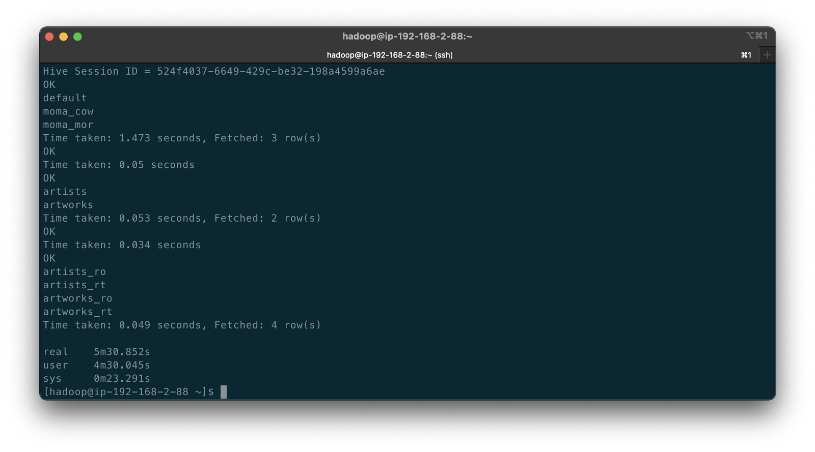
According to documentation, Hudi creates two tables in the Hive metastore for the MoR table type. The first, a table which is a read-optimized view appended with _ro and the second, a table with the same name appended with _rt which is a real-time view. According to Hudi, the read-optimized view exposes columnar Parquet while the real-time view exposes columnar Parquet and/or row-based logs; you can query both tables. The CoW table type creates a single table without a suffix for each datasource (e.g., artists). Below, we see the Hive table structure for the artists_rt table, created by DeltaStreamer, using SHOW CREATE TABLE moma_mor.artists_rt;.
Having run the demonstration’s deltastreamer_jobs_bulk_bkgd.sh script, the resulting object structure in the Hudi-managed section of the Amazon S3 bucket looks as follows.

Below is an example of Hudi files created in the /moma/artists_cow/ S3 object prefix. When using data lake table formats like Hudi, given its specialized directory structure and the high number of objects, interactions with the data should be abstracted through Hudi’s programming interfaces. Generally speaking, you do not interact directly with the objects in a data lake.
Hudi CLI
Optionally, we can inspect the Hudi tables using the Hudi CLI (hudi-cli). The CLI offers an extensive list of available commands. Using the CLI, we can inspect the Hudi tables and their schemas, and review operational statistics like write amplification (the number of bytes written for 1 byte of incoming data), commits, and compactions.
The following short video-only clip shows the use of the Hudi CLI, running on the Amazon EMR Master Node, to inspect the Hudi tables in S3.
Hudi Data Structure
Recall the sample Kafka message we saw earlier in the post representing an insert of an artist record with the artist_id 1. Below, we see what the same record looks like after being ingested by Hudi DeltaStreamer. Note the five additional fields added by Hudi with the _hoodie_ prefix.
Querying Hudi-managed Data
With the initial data ingestion complete and the CDC and DeltaStreamer processes monitoring for future changes, we can query the resulting data stored in Hudi tables. First, we will make some changes to the PostgreSQL MoMA Collection database to see how Hudi manages the data mutations. We could also make changes directly to the Hudi tables using Hive, Spark, or Presto. However, that would cause our datasource to be out of sync with the Hudi tables, potentially negating the entire CDC process. When developing a data lake, this is a critically important consideration — how changes are introduced to Hudi tables, especially when CDC is involved, and whether data continuity between datasources and the data lake is essential.
For the demonstration, I have made a series of arbitrary updates to a piece of artwork in the MoMA Collection database, ‘Picador (La Pique)’ by Pablo Picasso.
Below, note the last four objects shown in S3. Judging by the file names and dates, we can see that the CDC process, using Kafka Connect, has picked up the four updates I made to the record in the database. The Source Connector first wrote the changes to Kafka. The Sink Connector then read those Kafka messages and wrote the data to Amazon S3 in Avro format, as shown below.

Looking again at S3, we can also observe that DeltaStreamer picked up the new CDC objects in Amazon S3 and wrote them to both the Hudi CoW and MoR tables. Note the file types shown below. Given Hudi’s MoR table type structure, Hudi first logged the changes to row-based delta files and later compacted them to produce a new version of the columnar-format Parquet file.

Querying Results from Apache Hive
There are several ways to query Hudi-managed data in S3. In this demonstration, they include against Apache Hive using the hive client from the command line, against Hive using Spark, and against the Hudi tables also using Spark. We could also install Presto on EMR to query the Hudi data directly or via Hive.
Querying the real-time artwork_rt table in Hive after we make each database change, we can observe the data in Hudi reflects the updates. Note that the value of the _hoodie_file_name field for the first three updates is a Hudi delta log file, while the value for the last update is a Parquet file. The Parquet file signifies compaction occurred between the fourth update was made, and the time the Hive query was executed. Lastly, note the type of operation (_op) indicates an update change (u) for all records.

Once all fours database updates are complete and compaction has occurred, we should observe identical results from all Hive tables. Below, note the _hoodie_file_name field for all three tables is a Parquet file. Logically, the Parquet file for the MoR read-optimized and real-time Hive tables is the same.

Had we queried the data previous to compaction, the results would have differed. Below we have three queries. I further updated the artwork record, changing the date field from 1959 to 1960. The read-optimized MoR table, artworks_ro, still reflects the original date value, 1959, before the update and prior to compaction. The real-time table,artworks_rt , reflects the latest update to the date field, 1960. Note that the value of the _hoodie_file_name field for the read-optimized table is a Parquet file, while the value for the real-time table (artworks_rt), the third and final query, is a delta log file. The delta log allows the real-time table to display the most current state of the data in Hudi.

Below are a few useful Hive commands to query the changes in Hudi.
Deletes with Hudi
In addition to inserts and updates (upserts), Apache Hudi can manage deletes. Hudi supports implementing two types of deletes on data stored in Hudi tables: soft deletes and hard deletes. Given this demonstration’s specific configuration for CDC and DeltaStreamer, we will use soft deletes. Soft deletes retain the record key and nullify the other field’s values. Hard deletes, a stronger form of deletion, physically remove any record trace from the Hudi table.
Below, we see the CDC record for the artist with artist_id 441. The event flattening single message transformation (SMT), used by the Debezium-based Kafka Connect Source Connector, adds the __deleted field with a value of true and nullifies all fields except the record’s key, artist_id, which is required.
Below, we see the same delete record for the artist with artist_id 441 in the Hudi MoR table. All the null fields have been removed.
Below, we see how the deleted record appears in the three Hive CoW and MoR artwork tables. Note the query results from the read-optimized MoR table, artworks_ro, contains two records — the original record (r) and the deleted record (d). The data is partitioned by nationality, and since the record was deleted, the nationality field is changed to null. In S3, Hudi represents this partition as nationality=default. The record now exists in two different Parquet files, within two separate partitions, something to be aware of when querying the read-optimized MoR table.

Time Travel
According to the documentation, Hudi has supported time travel queries since version 0.9.0. With time travel, you can query the previous state of your data. Time travel is particularly useful for use cases, including rollbacks, debugging, and audit history.
To demonstrate time travel queries in Hudi, we start by making some additional changes to the source database. For this demonstration, I made a series of five updates and finally a delete to the artist record with artist_id 299 in the PostgreSQL database over a few-hour period.
Once the CDC and DeltaStreamer ingestion processes are complete, we can use Hudi’s time travel query capability to view the state of data in Hudi at different points in time (instants). To do so, we need to provide an as.an.instant date/time value to Spark (see line 21 below).
Based on the time period in which I made the five updates and the delete, I have chosen six instants during that period where I want to examine the state of the record. Below is an example of the PySpark code from a Jupyter Notebook used to perform the six time travel queries against the Hudi MoR artist’s table.
Below, we see the results of the time travel queries. At each instant, we can observe the mutating state of the data in the Hudi MoR Artist’s table, including the initial bulk insert of the existing snapshot of data (r) and the delete record (d). Since the delete made in the PostgreSQL database was recorded as a soft delete in Hudi, as opposed to a hard delete, we are still able to retrieve the record at any instant.
In addition to time travel queries, Hudi also offers incremental queries and point in time queries.
Conclusion
Although this post only scratches the surface of the capabilities of Debezium and Hudi, you can see the power of CDC using Kafka Connect and Debezium, combined with Hudi, to build and manage open data lakes on AWS.
This blog represents my own viewpoints and not of my employer, Amazon Web Services (AWS). All product names, logos, and brands are the property of their respective owners.
-
You are currently browsing the archives for the Technology Consulting category.
Gary Stafford
AWS Area Principal Solutions Architect | 10x AWS Certified Pro | DevOps | Data/ML | Serverless | Polyglot Developer | Former ThoughtWorks and Accenture
