Posts Tagged SQL
Executing Amazon Athena Queries from JetBrains PyCharm
Posted by Gary A. Stafford in AWS, Big Data, Cloud, Python, Software Development, SQL on January 8, 2020
Amazon Athena
According to Amazon, Athena is an interactive query service that makes it easy to analyze data in Amazon S3 using standard SQL. Amazon Athena supports and works with a variety of popular data file formats, including CSV, JSON, Apache ORC, Apache Avro, and Apache Parquet.
The underlying technology behind Amazon Athena is Presto, the popular, open-source distributed SQL query engine for big data, created by Facebook. According to AWS, the Athena query engine is based on Presto 0.172. Athena is ideal for quick, ad-hoc querying, but it can also handle complex analysis, including large joins, window functions, and arrays. In addition to Presto, Athena also uses Apache Hive to define tables.

Athena Query Editor
In the previous post, Getting Started with Data Analysis on AWS using AWS Glue, Amazon Athena, and QuickSight, we used the Athena Query Editor to construct and test SQL queries against semi-structured data in an S3-based Data Lake. The Athena Query Editor has many of the basic features Data Engineers and Analysts expect, including SQL syntax highlighting, code auto-completion, and query formatting. Queries can be run directly from the Editor, saved for future reference, and query results downloaded. The Editor can convert SELECT queries to CREATE TABLE AS (CTAS) and CREATE VIEW AS statements. Access to AWS Glue data sources is also available from within the Editor.
Full-Featured IDE
Although the Athena Query Editor is fairly functional, many Engineers perform a majority of their software development work in a fuller-featured IDE. The choice of IDE may depend on one’s predominant programming language. According to the PYPL Index, the ten most popular, current IDEs are:
- Microsoft Visual Studio
- Android Studio
- Eclipse
- Visual Studio Code
- Apache NetBeans
- JetBrains PyCharm
- JetBrains IntelliJ
- Apple Xcode
- Sublime Text
- Atom
Within the domains of data science, big data analytics, and data analysis, languages such as SQL, Python, Java, Scala, and R are common. Although I work in a variety of IDEs, my go-to choices are JetBrains PyCharm for Python (including for PySpark and Jupyter Notebook development) and JetBrains IntelliJ for Java and Scala (including Apache Spark development). Both these IDEs also support many common SQL-based technologies, out-of-the-box, and are easily extendable to add new technologies.

Athena Integration with PyCharm
Utilizing the extensibility of the JetBrains suite of professional development IDEs, it is simple to add Amazon Athena to the list of available database drivers and make JDBC (Java Database Connectivity) connections to Athena instances on AWS.
Downloading the Athena JDBC Driver
To start, download the Athena JDBC Driver from Amazon. There are two versions, based on your choice of Java JDKs. Considering Java 8 was released six years ago (March 2014), most users will likely want the AthenaJDBC42-2.0.9.jar is compatible with JDBC 4.2 and JDK 8.0 or later.

Installation Guide
AWS also supplies a JDBC Driver Installation and Configuration Guide. The guide, as well as the Athena JDBC and ODBC Drivers, are produced by Simba Technologies (acquired by Magnitude Software). Instructions for creating an Athena Driver starts on page 23.

Creating a New Athena Driver
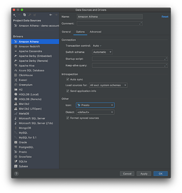
From PyCharm’s Database Tool Window, select the Drivers dialog box, select the downloaded Athena JDBC Driver JAR. Select com.simba.athena.jdbc.Driver in the Class dropdown. Name the Driver, ‘Amazon Athena.’

You can configure the Athena Driver further, using the Options and Advanced tabs.
Creating a New Athena Data Source
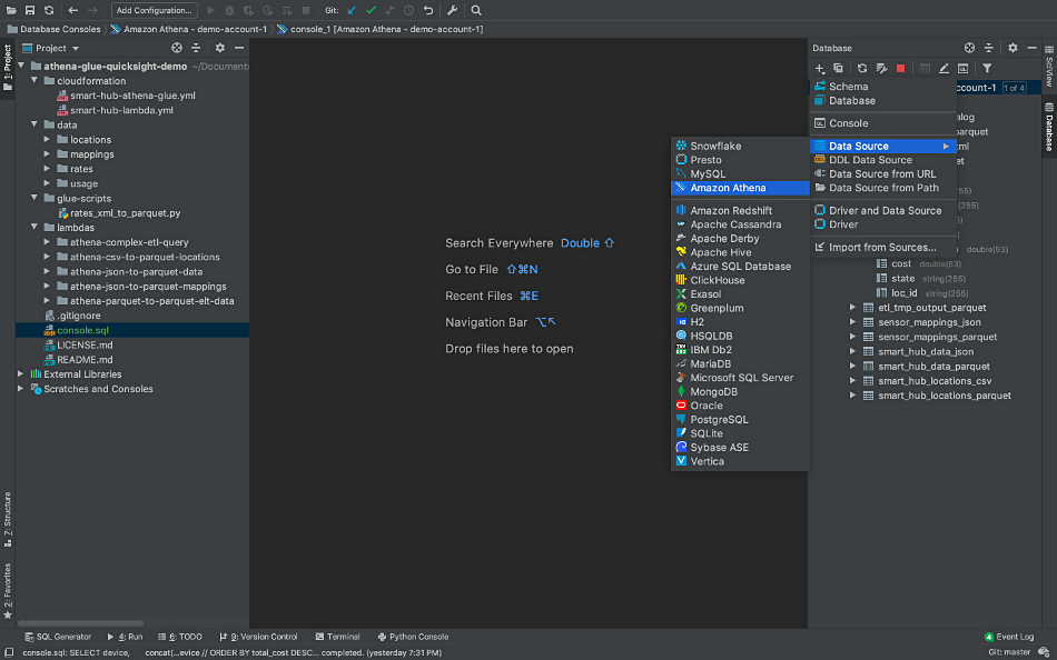
From PyCharm’s Database Tool Window, select the Data Source dialog box to create a new connection to your Athena instance. Choose ‘Amazon Athena’ from the list of available Database Drivers.
You will need four items to create an Athena Data Source:
- Your IAM User Access Key ID
- Your IAM User Secret Access Key
- The AWS Region of your Athena instance (e.g., us-east-1)
- An existing S3 bucket location to store query results
The Athena connection URL is a combination of the AWS Region and the S3 bucket, items 3 and 4, above. The format of the Athena connection URL is as follows.
jdbc:awsathena://AwsRegion=your-region;S3OutputLocation=s3://your-bucket-name/query-results-path
Give the new Athena Data Source a logical Name, input the User (Access Key ID), Password (Secret Access Key), and the Athena URL. To test the Athena Data Source, use the ‘Test Connection’ button.

You can create multiple Athena Data Sources using the Athena Driver. For example, you may have separate Development, Test, and Production instances of Athena, each in a different AWS Account.
Data Access
Once a successful connection has been made, switching to the Schemas tab, you should see a list of available AWS Glue Data Catalog databases. Below, we see the AWS Glue Catalog, which we created in the prior post. This Glue Data Catalog database contains ten metadata tables, each corresponding to a semi-structured, file-based data source in an S3-based data lake.
In the example below, I have chosen to limit the new Athena Data Source to a single Data Catalog database, to which the Data Source’s IAM User has access. Applying the core AWS security principle of granting least privilege, IAM Users should only have the permissions required to perform a specific set of approved tasks. This principle applies to the Glue Data Catalog databases, metadata tables, and the underlying S3 data sources.

Querying Athena from PyCharm
From within the PyCharm’s Database Tool Window, you should now see a list of the metadata tables defined in your AWS Glue Data Catalog database(s), as well as the individual columns within each table.

Similar to the Athena Query Editor, you can write SQL queries against the database tables in PyCharm. Like the Athena Query Editor, PyCharm has standard features SQL syntax highlighting, code auto-completion, and query formatting. Right-click on the Athena Data Source and choose New, then Console, to start.

Be mindful when writing queries and searching the Internet for SQL references, the Athena query engine is based on Presto 0.172. The current version of Presto, 0.234, is more than 50 releases ahead of the current Athena version. Both Athena and Presto functionality continue to change and diverge. There are also additional considerations and limitations for SQL queries in Athena to be aware of.
Whereas the Athena Query Editor is limited to only one query per query tab, in PyCharm, we can write and run multiple SQL queries in the same console window and have multiple console sessions opened to Athena at the same time.

By default, PyCharm’s query results are limited to the first ten rows of data. The number of rows displayed, as well as many other preferences, can be changed in the PyCharm’s Database Preferences dialog box.

Saving Queries and Exporting Results
In PyCharm, Athena queries can be saved as part of your PyCharm projects, as .sql files. Whereas the Athena Query Editor is limited to CSV, in PyCharm, query results can be exported in a variety of standard data file formats.

Athena Query History
All Athena queries ran from PyCharm are recorded in the History tab of the Athena Console. Although PyCharm shows query run times, the Athena History tab also displays the amount of data scanned. Knowing the query run time and volume of data scanned is useful when performance tuning queries.

Other IDEs
The technique shown for JetBrains PyCharm can also be applied to other JetBrains products, including GoLand, DataGrip, PhpStorm, and IntelliJ (shown below).

This blog represents my own view points and not of my employer, Amazon Web Services.
Getting Started with Data Analysis on AWS using AWS Glue, Amazon Athena, and QuickSight: Part 1
Posted by Gary A. Stafford in AWS, Bash Scripting, Big Data, Cloud, Python, Serverless, Software Development on January 5, 2020
Introduction
According to Wikipedia, data analysis is “a process of inspecting, cleansing, transforming, and modeling data with the goal of discovering useful information, informing conclusion, and supporting decision-making.” In this two-part post, we will explore how to get started with data analysis on AWS, using the serverless capabilities of Amazon Athena, AWS Glue, Amazon QuickSight, Amazon S3, and AWS Lambda. We will learn how to use these complementary services to transform, enrich, analyze, and visualize semi-structured data.
Data Analysis—discovering useful information, informing conclusion, and supporting decision-making. –Wikipedia
In part one, we will begin with raw, semi-structured data in multiple formats. We will discover how to ingest, transform, and enrich that data using Amazon S3, AWS Glue, Amazon Athena, and AWS Lambda. We will build an S3-based data lake, and learn how AWS leverages open-source technologies, such as Presto, Apache Hive, and Apache Parquet. In part two, we will learn how to further analyze and visualize the data using Amazon QuickSight. Here’s a quick preview of what we will build in part one of the post.
Demonstration
In this demonstration, we will adopt the persona of a large, US-based electric energy provider. The energy provider has developed its next-generation Smart Electrical Monitoring Hub (Smart Hub). They have sold the Smart Hub to a large number of residential customers throughout the United States. The hypothetical Smart Hub wirelessly collects detailed electrical usage data from individual, smart electrical receptacles and electrical circuit meters, spread throughout the residence. Electrical usage data is encrypted and securely transmitted from the customer’s Smart Hub to the electric provider, who is running their business on AWS.
Customers are able to analyze their electrical usage with fine granularity, per device, and over time. The goal of the Smart Hub is to enable the customers, using data, to reduce their electrical costs. The provider benefits from a reduction in load on the existing electrical grid and a better distribution of daily electrical load as customers shift usage to off-peak times to save money.
 Preview of post’s data in Amazon QuickSight.
The original concept for the Smart Hub was developed as part of a multi-day training and hackathon, I recently attended with an AWSome group of AWS Solutions Architects in San Francisco. As a team, we developed the concept of the Smart Hub integrated with a real-time, serverless, streaming data architecture, leveraging AWS IoT Core, Amazon Kinesis, AWS Lambda, and Amazon DynamoDB.
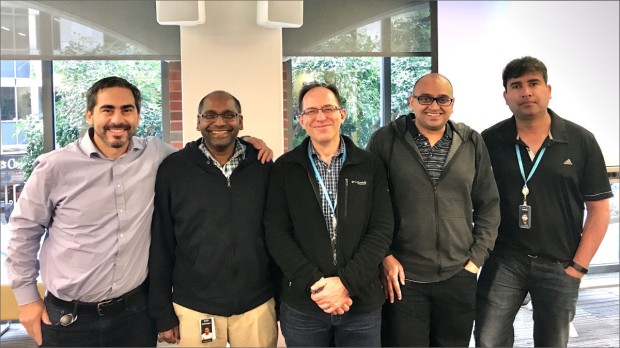 From left: Bruno Giorgini, Mahalingam (‘Mahali’) Sivaprakasam, Gary Stafford, Amit Kumar Agrawal, and Manish Agarwal.
This post will focus on data analysis, as opposed to the real-time streaming aspect of data capture or how the data is persisted on AWS.
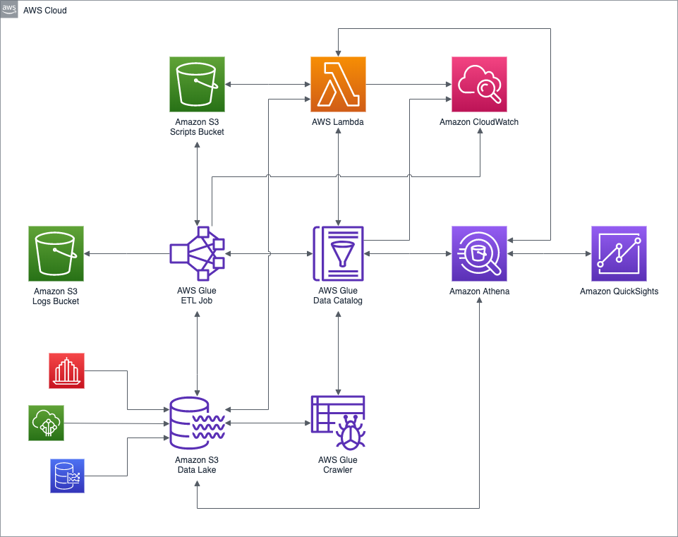 High-level AWS architecture diagram of the demonstration.
Featured Technologies
The following AWS services and open-source technologies are featured prominently in this post.

Amazon S3-based Data Lake
 An Amazon S3-based Data Lake uses Amazon S3 as its primary storage platform. Amazon S3 provides an optimal foundation for a data lake because of its virtually unlimited scalability, from gigabytes to petabytes of content. Amazon S3 provides ‘11 nines’ (99.999999999%) durability. It has scalable performance, ease-of-use features, and native encryption and access control capabilities.
AWS Glue
 AWS Glue is a fully managed extract, transform, and load (ETL) service to prepare and load data for analytics. AWS Glue discovers your data and stores the associated metadata (e.g., table definition and schema) in the AWS Glue Data Catalog. Once cataloged, your data is immediately searchable, queryable, and available for ETL.
AWS Glue Data Catalog
 The AWS Glue Data Catalog is an Apache Hive Metastore compatible, central repository to store structural and operational metadata for data assets. For a given data set, store table definition, physical location, add business-relevant attributes, as well as track how the data has changed over time.
AWS Glue Crawler
 An AWS Glue Crawler connects to a data store, progresses through a prioritized list of classifiers to extract the schema of your data and other statistics, and then populates the Glue Data Catalog with this metadata. Crawlers can run periodically to detect the availability of new data as well as changes to existing data, including table definition changes. Crawlers automatically add new tables, new partitions to an existing table, and new versions of table definitions. You can even customize Glue Crawlers to classify your own file types.
AWS Glue ETL Job
 An AWS Glue ETL Job is the business logic that performs extract, transform, and load (ETL) work in AWS Glue. When you start a job, AWS Glue runs a script that extracts data from sources, transforms the data, and loads it into targets. AWS Glue generates a PySpark or Scala script, which runs on Apache Spark.
Amazon Athena
 Amazon Athena is an interactive query service that makes it easy to analyze data in Amazon S3 using standard SQL. Athena supports and works with a variety of standard data formats, including CSV, JSON, Apache ORC, Apache Avro, and Apache Parquet. Athena is integrated, out-of-the-box, with AWS Glue Data Catalog. Athena is serverless, so there is no infrastructure to manage, and you pay only for the queries that you run.
The underlying technology behind Amazon Athena is Presto, the open-source distributed SQL query engine for big data, created by Facebook. According to the AWS, the Athena query engine is based on Presto 0.172 (released April 9, 2017). In addition to Presto, Athena uses Apache Hive to define tables.
Amazon QuickSight
 Amazon QuickSight is a fully managed business intelligence (BI) service. QuickSight lets you create and publish interactive dashboards that can then be accessed from any device, and embedded into your applications, portals, and websites.
AWS Lambda
 AWS Lambda automatically runs code without requiring the provisioning or management servers. AWS Lambda automatically scales applications by running code in response to triggers. Lambda code runs in parallel. With AWS Lambda, you are charged for every 100ms your code executes and the number of times your code is triggered. You pay only for the compute time you consume.
Smart Hub Data
Everything in this post revolves around data. For the post’s demonstration, we will start with four categories of raw, synthetic data. Those data categories include Smart Hub electrical usage data, Smart Hub sensor mapping data, Smart Hub residential locations data, and electrical rate data. To demonstrate the capabilities of AWS Glue to handle multiple data formats, the four categories of raw data consist of three distinct file formats: XML, JSON, and CSV. I have attempted to incorporate as many ‘real-world’ complexities into the data without losing focus on the main subject of the post. The sample datasets are intentionally small to keep your AWS costs to a minimum for the demonstration.
To further reduce costs, we will use a variety of data partitioning schemes. According to AWS, by partitioning your data, you can restrict the amount of data scanned by each query, thus improving performance and reducing cost. We have very little data for the demonstration, in which case partitioning may negatively impact query performance. However, in a ‘real-world’ scenario, there would be millions of potential residential customers generating terabytes of data. In that case, data partitioning would be essential for both cost and performance.
Smart Hub Electrical Usage Data
The Smart Hub’s time-series electrical usage data is collected from the customer’s Smart Hub. In the demonstration’s sample electrical usage data, each row represents a completely arbitrary five-minute time interval. There are a total of ten electrical sensors whose electrical usage in kilowatt-hours (kW) is recorded and transmitted. Each Smart Hub records and transmits electrical usage for 10 device sensors, 288 times per day (24 hr / 5 min intervals), for a total of 2,880 data points per day, per Smart Hub. There are two days worth of usage data for the demonstration, for a total of 5,760 data points. The data is stored in JSON Lines format. The usage data will be partitioned in the Amazon S3-based data lake by date (e.g., ‘dt=2019-12-21’).
This file contains bidirectional Unicode text that may be interpreted or compiled differently than what appears below. To review, open the file in an editor that reveals hidden Unicode characters.
Learn more about bidirectional Unicode characters
| {"loc_id":"b6a8d42425fde548","ts":1576915200,"data":{"s_01":0,"s_02":0.00502,"s_03":0,"s_04":0,"s_05":0,"s_06":0,"s_07":0,"s_08":0,"s_09":0,"s_10":0.04167}} | |
| {"loc_id":"b6a8d42425fde548","ts":1576915500,"data":{"s_01":0,"s_02":0.00552,"s_03":0,"s_04":0,"s_05":0,"s_06":0,"s_07":0,"s_08":0,"s_09":0,"s_10":0.04147}} | |
| {"loc_id":"b6a8d42425fde548","ts":1576915800,"data":{"s_01":0.29267,"s_02":0.00642,"s_03":0,"s_04":0,"s_05":0,"s_06":0,"s_07":0,"s_08":0,"s_09":0,"s_10":0.04207}} | |
| {"loc_id":"b6a8d42425fde548","ts":1576916100,"data":{"s_01":0.29207,"s_02":0.00592,"s_03":0,"s_04":0,"s_05":0,"s_06":0,"s_07":0,"s_08":0,"s_09":0,"s_10":0.04137}} | |
| {"loc_id":"b6a8d42425fde548","ts":1576916400,"data":{"s_01":0.29217,"s_02":0.00622,"s_03":0,"s_04":0,"s_05":0,"s_06":0,"s_07":0,"s_08":0,"s_09":0,"s_10":0.04157}} | |
| {"loc_id":"b6a8d42425fde548","ts":1576916700,"data":{"s_01":0,"s_02":0.00562,"s_03":0,"s_04":0,"s_05":0,"s_06":0,"s_07":0,"s_08":0,"s_09":0,"s_10":0.04197}} | |
| {"loc_id":"b6a8d42425fde548","ts":1576917000,"data":{"s_01":0,"s_02":0.00512,"s_03":0,"s_04":0,"s_05":0,"s_06":0,"s_07":0,"s_08":0,"s_09":0,"s_10":0.04257}} | |
| {"loc_id":"b6a8d42425fde548","ts":1576917300,"data":{"s_01":0,"s_02":0.00522,"s_03":0,"s_04":0,"s_05":0,"s_06":0,"s_07":0,"s_08":0,"s_09":0,"s_10":0.04177}} | |
| {"loc_id":"b6a8d42425fde548","ts":1576917600,"data":{"s_01":0,"s_02":0.00502,"s_03":0,"s_04":0,"s_05":0,"s_06":0,"s_07":0,"s_08":0,"s_09":0,"s_10":0.04267}} | |
| {"loc_id":"b6a8d42425fde548","ts":1576917900,"data":{"s_01":0,"s_02":0.00612,"s_03":0,"s_04":0,"s_05":0,"s_06":0,"s_07":0,"s_08":0,"s_09":0,"s_10":0.04237}} |
Note the electrical usage data contains nested data. The electrical usage for each of the ten sensors is contained in a JSON array, within each time series entry. The array contains ten numeric values of type, double.
This file contains bidirectional Unicode text that may be interpreted or compiled differently than what appears below. To review, open the file in an editor that reveals hidden Unicode characters.
Learn more about bidirectional Unicode characters
| { | |
| "loc_id": "b6a8d42425fde548", | |
| "ts": 1576916400, | |
| "data": { | |
| "s_01": 0.29217, | |
| "s_02": 0.00622, | |
| "s_03": 0, | |
| "s_04": 0, | |
| "s_05": 0, | |
| "s_06": 0, | |
| "s_07": 0, | |
| "s_08": 0, | |
| "s_09": 0, | |
| "s_10": 0.04157 | |
| } | |
| } |
Real data is often complex and deeply nested. Later in the post, we will see that AWS Glue can map many common data types, including nested data objects, as illustrated below.

Smart Hub Sensor Mappings
The Smart Hub sensor mappings data maps a sensor column in the usage data (e.g., ‘s_01’ to the corresponding actual device (e.g., ‘Central Air Conditioner’). The data contains the device location, wattage, and the last time the record was modified. The data is also stored in JSON Lines format. The sensor mappings data will be partitioned in the Amazon S3-based data lake by the state of the residence (e.g., ‘state=or’ for Oregon).
This file contains bidirectional Unicode text that may be interpreted or compiled differently than what appears below. To review, open the file in an editor that reveals hidden Unicode characters.
Learn more about bidirectional Unicode characters
| {"loc_id":"b6a8d42425fde548","id":"s_01","description":"Central Air Conditioner","location":"N/A","watts":3500,"last_modified":1559347200} | |
| {"loc_id":"b6a8d42425fde548","id":"s_02","description":"Ceiling Fan","location":"Master Bedroom","watts":65,"last_modified":1559347200} | |
| {"loc_id":"b6a8d42425fde548","id":"s_03","description":"Clothes Dryer","location":"Basement","watts":5000,"last_modified":1559347200} | |
| {"loc_id":"b6a8d42425fde548","id":"s_04","description":"Clothes Washer","location":"Basement","watts":1800,"last_modified":1559347200} | |
| {"loc_id":"b6a8d42425fde548","id":"s_05","description":"Dishwasher","location":"Kitchen","watts":900,"last_modified":1559347200} | |
| {"loc_id":"b6a8d42425fde548","id":"s_06","description":"Flat Screen TV","location":"Living Room","watts":120,"last_modified":1559347200} | |
| {"loc_id":"b6a8d42425fde548","id":"s_07","description":"Microwave Oven","location":"Kitchen","watts":1000,"last_modified":1559347200} | |
| {"loc_id":"b6a8d42425fde548","id":"s_08","description":"Coffee Maker","location":"Kitchen","watts":900,"last_modified":1559347200} | |
| {"loc_id":"b6a8d42425fde548","id":"s_09","description":"Hair Dryer","location":"Master Bathroom","watts":2000,"last_modified":1559347200} | |
| {"loc_id":"b6a8d42425fde548","id":"s_10","description":"Refrigerator","location":"Kitchen","watts":500,"last_modified":1559347200} |
Smart Hub Locations
The Smart Hub locations data contains the geospatial coordinates, home address, and timezone for each residential Smart Hub. The data is stored in CSV format. The data for the four cities included in this demonstration originated from OpenAddresses, ‘the free and open global address collection.’ There are approximately 4k location records. The location data will be partitioned in the Amazon S3-based data lake by the state of the residence where the Smart Hub is installed (e.g., ‘state=or’ for Oregon).
This file contains bidirectional Unicode text that may be interpreted or compiled differently than what appears below. To review, open the file in an editor that reveals hidden Unicode characters.
Learn more about bidirectional Unicode characters
| lon | lat | number | street | unit | city | district | region | postcode | id | hash | tz | |
|---|---|---|---|---|---|---|---|---|---|---|---|---|
| -122.8077278 | 45.4715614 | 6635 | SW JUNIPER TER | 97008 | b6a8d42425fde548 | America/Los_Angeles | ||||||
| -122.8356634 | 45.4385864 | 11225 | SW PINTAIL LOOP | 97007 | 08ae3df798df8b90 | America/Los_Angeles | ||||||
| -122.8252379 | 45.4481709 | 9930 | SW WRANGLER PL | 97008 | 1c7e1f7df752663e | America/Los_Angeles | ||||||
| -122.8354211 | 45.4535977 | 9174 | SW PLATINUM PL | 97007 | b364854408ee431e | America/Los_Angeles | ||||||
| -122.8315771 | 45.4949449 | 15040 | SW MILLIKAN WAY | # 233 | 97003 | 0e97796ba31ba3b4 | America/Los_Angeles | |||||
| -122.7950339 | 45.4470259 | 10006 | SW CONESTOGA DR | # 113 | 97008 | 2b5307be5bfeb026 | America/Los_Angeles | |||||
| -122.8072836 | 45.4908594 | 12600 | SW CRESCENT ST | # 126 | 97005 | 4d74167f00f63f50 | America/Los_Angeles | |||||
| -122.8211801 | 45.4689303 | 7100 | SW 140TH PL | 97008 | c5568631f0b9de9c | America/Los_Angeles | ||||||
| -122.831154 | 45.4317057 | 15050 | SW MALLARD DR | # 101 | 97007 | dbd1321080ce9682 | America/Los_Angeles | |||||
| -122.8162856 | 45.4442878 | 10460 | SW 136TH PL | 97008 | 008faab8a9a3e519 | America/Los_Angeles |
Electrical Rates
Lastly, the electrical rate data contains the cost of electricity. In this demonstration, the assumption is that the rate varies by state, by month, and by the hour of the day. The data is stored in XML, a data export format still common to older, legacy systems. The electrical rate data will not be partitioned in the Amazon S3-based data lake.
This file contains bidirectional Unicode text that may be interpreted or compiled differently than what appears below. To review, open the file in an editor that reveals hidden Unicode characters.
Learn more about bidirectional Unicode characters
| <?xml version="1.0" encoding="UTF-8"?> | |
| <root> | |
| <row> | |
| <state>or</state> | |
| <year>2019</year> | |
| <month>12</month> | |
| <from>19:00:00</from> | |
| <to>19:59:59</to> | |
| <type>peak</type> | |
| <rate>12.623</rate> | |
| </row> | |
| <row> | |
| <state>or</state> | |
| <year>2019</year> | |
| <month>12</month> | |
| <from>20:00:00</from> | |
| <to>20:59:59</to> | |
| <type>partial-peak</type> | |
| <rate>7.232</rate> | |
| </row> | |
| <row> | |
| <state>or</state> | |
| <year>2019</year> | |
| <month>12</month> | |
| <from>21:00:00</from> | |
| <to>21:59:59</to> | |
| <type>partial-peak</type> | |
| <rate>7.232</rate> | |
| </row> | |
| <row> | |
| <state>or</state> | |
| <year>2019</year> | |
| <month>12</month> | |
| <from>22:00:00</from> | |
| <to>22:59:59</to> | |
| <type>off-peak</type> | |
| <rate>4.209</rate> | |
| </row> | |
| </root> |
Data Analysis Process
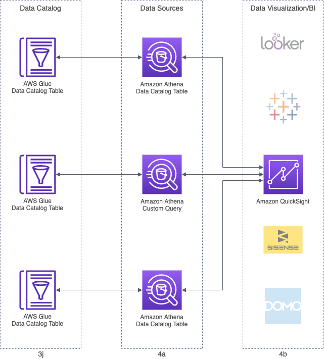
Due to the number of steps involved in the data analysis process in the demonstration, I have divided the process into four logical stages: 1) Raw Data Ingestion, 2) Data Transformation, 3) Data Enrichment, and 4) Data Visualization and Business Intelligence (BI).
 Full data analysis workflow diagram (click to enlarge…)
Raw Data Ingestion
In the Raw Data Ingestion stage, semi-structured CSV-, XML-, and JSON-format data files are copied to a secure Amazon Simple Storage Service (S3) bucket. Within the bucket, data files are organized into folders based on their physical data structure (schema). Due to the potentially unlimited number of data files, files are further organized (partitioned) into subfolders. Organizational strategies for data files are based on date, time, geographic location, customer id, or other common data characteristics.
This collection of semi-structured data files, S3 buckets, and partitions form what is referred to as a Data Lake. According to AWS, a data lake is a centralized repository that allows you to store all your structured and unstructured data at any scale.
A series of AWS Glue Crawlers process the raw CSV-, XML-, and JSON-format files, extracting metadata, and creating table definitions in the AWS Glue Data Catalog. According to AWS, an AWS Glue Data Catalog contains metadata tables, where each table specifies a single data store.

Data Transformation
In the Data Transformation stage, the raw data in the previous stage is transformed. Data transformation may include both modifying the data and changing the data format. Data modifications include data cleansing, re-casting data types, changing date formats, field-level computations, and field concatenation.
The data is then converted from CSV-, XML-, and JSON-format to Apache Parquet format and written back to the Amazon S3-based data lake. Apache Parquet is a compressed, efficient columnar storage format. Amazon Athena, like many Cloud-based services, charges you by the amount of data scanned per query. Hence, using data partitioning, bucketing, compression, and columnar storage formats, like Parquet, will reduce query cost.
Lastly, the transformed Parquet-format data is cataloged to new tables, alongside the raw CSV, XML, and JSON data, in the Glue Data Catalog.

Data Enrichment
According to ScienceDirect, data enrichment or augmentation is the process of enhancing existing information by supplementing missing or incomplete data. Typically, data enrichment is achieved by using external data sources, but that is not always the case.
Data Enrichment—the process of enhancing existing information by supplementing missing or incomplete data. –ScienceDirect
In the Data Enrichment stage, the Parquet-format Smart Hub usage data is augmented with related data from the three other data sources: sensor mappings, locations, and electrical rates. The customer’s Smart Hub usage data is enriched with the customer’s device types, the customer’s timezone, and customer’s electricity cost per monitored period based on the customer’s geographic location and time of day.

Once the data is enriched, it is converted to Parquet and optimized for query performance, stored in the data lake, and cataloged. At this point, the original CSV-, XML-, and JSON-format raw data files, the transformed Parquet-format data files, and the Parquet-format enriched data files are all stored in the Amazon S3-based data lake and cataloged in the Glue Data Catalog.

Data Visualization
In the final Data Visualization and Business Intelligence (BI) stage, the enriched data is presented and analyzed. There are many enterprise-grade services available for visualization and Business Intelligence, which integrate with Athena. Amazon services include Amazon QuickSight, Amazon EMR, and Amazon SageMaker. Third-party solutions from AWS Partners, available on the AWS Marketplace, include Tableau, Looker, Sisense, and Domo. In this demonstration, we will focus on Amazon QuickSight.
Getting Started
Requirements
To follow along with the demonstration, you will need an AWS Account and a current version of the AWS CLI. To get the most from the demonstration, you should also have Python 3 and jq installed in your work environment.
Source Code
All source code for this post can be found on GitHub. Use the following command to clone a copy of the project.
This file contains bidirectional Unicode text that may be interpreted or compiled differently than what appears below. To review, open the file in an editor that reveals hidden Unicode characters.
Learn more about bidirectional Unicode characters
| git clone \ | |
| –branch master –single-branch –depth 1 –no-tags \ | |
| https://github.com/garystafford/athena-glue-quicksight-demo.git |
Source code samples in this post are displayed as GitHub Gists, which will not display correctly on some mobile and social media browsers.
TL;DR?
Just want the jump in without reading the instructions? All the AWS CLI commands, found within the post, are consolidated in the GitHub project’s README file.
CloudFormation Stack
To start, create the ‘smart-hub-athena-glue-stack’ CloudFormation stack using the smart-hub-athena-glue.yml template. The template will create (3) Amazon S3 buckets, (1) AWS Glue Data Catalog Database, (5) Data Catalog Database Tables, (6) AWS Glue Crawlers, (1) AWS Glue ETL Job, and (1) IAM Service Role for AWS Glue.
Make sure to change the DATA_BUCKET, SCRIPT_BUCKET, and LOG_BUCKET variables, first, to your own unique S3 bucket names. I always suggest using the standard AWS 3-part convention of 1) descriptive name, 2) AWS Account ID or Account Alias, and 3) AWS Region, to name your bucket (e.g. ‘smart-hub-data-123456789012-us-east-1’).
This file contains bidirectional Unicode text that may be interpreted or compiled differently than what appears below. To review, open the file in an editor that reveals hidden Unicode characters.
Learn more about bidirectional Unicode characters
| # *** CHANGE ME *** | |
| BUCKET_SUFFIX="123456789012-us-east-1" | |
| DATA_BUCKET="smart-hub-data-${BUCKET_SUFFIX}" | |
| SCRIPT_BUCKET="smart-hub-scripts-${BUCKET_SUFFIX}" | |
| LOG_BUCKET="smart-hub-logs-${BUCKET_SUFFIX}" | |
| aws cloudformation create-stack \ | |
| –stack-name smart-hub-athena-glue-stack \ | |
| –template-body file://cloudformation/smart-hub-athena-glue.yml \ | |
| –parameters ParameterKey=DataBucketName,ParameterValue=${DATA_BUCKET} \ | |
| ParameterKey=ScriptBucketName,ParameterValue=${SCRIPT_BUCKET} \ | |
| ParameterKey=LogBucketName,ParameterValue=${LOG_BUCKET} \ | |
| –capabilities CAPABILITY_NAMED_IAM |
Raw Data Files
Next, copy the raw CSV-, XML-, and JSON-format data files from the local project to the DATA_BUCKET S3 bucket (steps 1a-1b in workflow diagram). These files represent the beginnings of the S3-based data lake. Each category of data uses a different strategy for organizing and separating the files. Note the use of the Apache Hive-style partitions (e.g., /smart_hub_data_json/dt=2019-12-21). As discussed earlier, the assumption is that the actual, large volume of data in the data lake would necessitate using partitioning to improve query performance.
This file contains bidirectional Unicode text that may be interpreted or compiled differently than what appears below. To review, open the file in an editor that reveals hidden Unicode characters.
Learn more about bidirectional Unicode characters
| # location data | |
| aws s3 cp data/locations/denver_co_1576656000.csv \ | |
| s3://${DATA_BUCKET}/smart_hub_locations_csv/state=co/ | |
| aws s3 cp data/locations/palo_alto_ca_1576742400.csv \ | |
| s3://${DATA_BUCKET}/smart_hub_locations_csv/state=ca/ | |
| aws s3 cp data/locations/portland_metro_or_1576742400.csv \ | |
| s3://${DATA_BUCKET}/smart_hub_locations_csv/state=or/ | |
| aws s3 cp data/locations/stamford_ct_1576569600.csv \ | |
| s3://${DATA_BUCKET}/smart_hub_locations_csv/state=ct/ | |
| # sensor mapping data | |
| aws s3 cp data/mappings/ \ | |
| s3://${DATA_BUCKET}/sensor_mappings_json/state=or/ \ | |
| –recursive | |
| # electrical usage data | |
| aws s3 cp data/usage/2019-12-21/ \ | |
| s3://${DATA_BUCKET}/smart_hub_data_json/dt=2019-12-21/ \ | |
| –recursive | |
| aws s3 cp data/usage/2019-12-22/ \ | |
| s3://${DATA_BUCKET}/smart_hub_data_json/dt=2019-12-22/ \ | |
| –recursive | |
| # electricity rates data | |
| aws s3 cp data/rates/ \ | |
| s3://${DATA_BUCKET}/electricity_rates_xml/ \ | |
| –recursive |
Confirm the contents of the DATA_BUCKET S3 bucket with the following command.
This file contains bidirectional Unicode text that may be interpreted or compiled differently than what appears below. To review, open the file in an editor that reveals hidden Unicode characters.
Learn more about bidirectional Unicode characters
| aws s3 ls s3://${DATA_BUCKET}/ \ | |
| –recursive –human-readable –summarize |
There should be a total of (14) raw data files in the DATA_BUCKET S3 bucket.
This file contains bidirectional Unicode text that may be interpreted or compiled differently than what appears below. To review, open the file in an editor that reveals hidden Unicode characters.
Learn more about bidirectional Unicode characters
| 2020-01-04 14:39:51 20.0 KiB electricity_rates_xml/2019_12_1575270000.xml | |
| 2020-01-04 14:39:46 1.3 KiB sensor_mappings_json/state=or/08ae3df798df8b90_1550908800.json | |
| 2020-01-04 14:39:46 1.3 KiB sensor_mappings_json/state=or/1c7e1f7df752663e_1559347200.json | |
| 2020-01-04 14:39:46 1.3 KiB sensor_mappings_json/state=or/b6a8d42425fde548_1568314800.json | |
| 2020-01-04 14:39:47 44.9 KiB smart_hub_data_json/dt=2019-12-21/08ae3df798df8b90_1576915200.json | |
| 2020-01-04 14:39:47 44.9 KiB smart_hub_data_json/dt=2019-12-21/1c7e1f7df752663e_1576915200.json | |
| 2020-01-04 14:39:47 44.9 KiB smart_hub_data_json/dt=2019-12-21/b6a8d42425fde548_1576915200.json | |
| 2020-01-04 14:39:49 44.6 KiB smart_hub_data_json/dt=2019-12-22/08ae3df798df8b90_15770016000.json | |
| 2020-01-04 14:39:49 44.6 KiB smart_hub_data_json/dt=2019-12-22/1c7e1f7df752663e_1577001600.json | |
| 2020-01-04 14:39:49 44.6 KiB smart_hub_data_json/dt=2019-12-22/b6a8d42425fde548_15770016001.json | |
| 2020-01-04 14:39:39 89.7 KiB smart_hub_locations_csv/state=ca/palo_alto_ca_1576742400.csv | |
| 2020-01-04 14:39:37 84.2 KiB smart_hub_locations_csv/state=co/denver_co_1576656000.csv | |
| 2020-01-04 14:39:44 78.6 KiB smart_hub_locations_csv/state=ct/stamford_ct_1576569600.csv | |
| 2020-01-04 14:39:42 91.6 KiB smart_hub_locations_csv/state=or/portland_metro_or_1576742400.csv | |
| Total Objects: 14 | |
| Total Size: 636.7 KiB |
Lambda Functions
Next, package the (5) Python3.8-based AWS Lambda functions for deployment.
This file contains bidirectional Unicode text that may be interpreted or compiled differently than what appears below. To review, open the file in an editor that reveals hidden Unicode characters.
Learn more about bidirectional Unicode characters
| pushd lambdas/athena-json-to-parquet-data || exit | |
| zip -r package.zip index.py | |
| popd || exit | |
| pushd lambdas/athena-csv-to-parquet-locations || exit | |
| zip -r package.zip index.py | |
| popd || exit | |
| pushd lambdas/athena-json-to-parquet-mappings || exit | |
| zip -r package.zip index.py | |
| popd || exit | |
| pushd lambdas/athena-complex-etl-query || exit | |
| zip -r package.zip index.py | |
| popd || exit | |
| pushd lambdas/athena-parquet-to-parquet-elt-data || exit | |
| zip -r package.zip index.py | |
| popd || exit |
Copy the five Lambda packages to the SCRIPT_BUCKET S3 bucket. The ZIP archive Lambda packages are accessed by the second CloudFormation stack, smart-hub-serverless. This CloudFormation stack, which creates the Lambda functions, will fail to deploy if the packages are not found in the SCRIPT_BUCKET S3 bucket.
I have chosen to place the packages in a different S3 bucket then the raw data files. In a real production environment, these two types of files would be separated, minimally, into separate buckets for security. Remember, only data should go into the data lake.
This file contains bidirectional Unicode text that may be interpreted or compiled differently than what appears below. To review, open the file in an editor that reveals hidden Unicode characters.
Learn more about bidirectional Unicode characters
| aws s3 cp lambdas/athena-json-to-parquet-data/package.zip \ | |
| s3://${SCRIPT_BUCKET}/lambdas/athena_json_to_parquet_data/ | |
| aws s3 cp lambdas/athena-csv-to-parquet-locations/package.zip \ | |
| s3://${SCRIPT_BUCKET}/lambdas/athena_csv_to_parquet_locations/ | |
| aws s3 cp lambdas/athena-json-to-parquet-mappings/package.zip \ | |
| s3://${SCRIPT_BUCKET}/lambdas/athena_json_to_parquet_mappings/ | |
| aws s3 cp lambdas/athena-complex-etl-query/package.zip \ | |
| s3://${SCRIPT_BUCKET}/lambdas/athena_complex_etl_query/ | |
| aws s3 cp lambdas/athena-parquet-to-parquet-elt-data/package.zip \ | |
| s3://${SCRIPT_BUCKET}/lambdas/athena_parquet_to_parquet_elt_data/ |
Create the second ‘smart-hub-lambda-stack’ CloudFormation stack using the smart-hub-lambda.yml CloudFormation template. The template will create (5) AWS Lambda functions and (1) Lambda execution IAM Service Role.
This file contains bidirectional Unicode text that may be interpreted or compiled differently than what appears below. To review, open the file in an editor that reveals hidden Unicode characters.
Learn more about bidirectional Unicode characters
| aws cloudformation create-stack \ | |
| –stack-name smart-hub-lambda-stack \ | |
| –template-body file://cloudformation/smart-hub-lambda.yml \ | |
| –capabilities CAPABILITY_NAMED_IAM |
At this point, we have deployed all of the AWS resources required for the demonstration using CloudFormation. We have also copied all of the raw CSV-, XML-, and JSON-format data files in the Amazon S3-based data lake.
AWS Glue Crawlers
If you recall, we created five tables in the Glue Data Catalog database as part of the CloudFormation stack. One table for each of the four raw data types and one table to hold temporary ELT data later in the demonstration. To confirm the five tables were created in the Glue Data Catalog database, use the Glue Data Catalog Console, or run the following AWS CLI / jq command.
This file contains bidirectional Unicode text that may be interpreted or compiled differently than what appears below. To review, open the file in an editor that reveals hidden Unicode characters.
Learn more about bidirectional Unicode characters
| aws glue get-tables \ | |
| –database-name smart_hub_data_catalog \ | |
| | jq -r '.TableList[].Name' |
The five data catalog tables should be as follows.
This file contains bidirectional Unicode text that may be interpreted or compiled differently than what appears below. To review, open the file in an editor that reveals hidden Unicode characters.
Learn more about bidirectional Unicode characters
| electricity_rates_xml | |
| etl_tmp_output_parquet | |
| sensor_mappings_json | |
| smart_hub_data_json | |
| smart_hub_locations_csv |
We also created six Glue Crawlers as part of the CloudFormation template. Four of these Crawlers are responsible for cataloging the raw CSV-, XML-, and JSON-format data from S3 into the corresponding, existing Glue Data Catalog database tables. The Crawlers will detect any new partitions and add those to the tables as well. Each Crawler corresponds to one of the four raw data types. Crawlers can be scheduled to run periodically, cataloging new data and updating data partitions. Crawlers will also create a Data Catalog database tables. We use Crawlers to create new tables, later in the post.
Run the four Glue Crawlers using the AWS CLI (step 1c in workflow diagram).
This file contains bidirectional Unicode text that may be interpreted or compiled differently than what appears below. To review, open the file in an editor that reveals hidden Unicode characters.
Learn more about bidirectional Unicode characters
| aws glue start-crawler –name smart-hub-locations-csv | |
| aws glue start-crawler –name smart-hub-sensor-mappings-json | |
| aws glue start-crawler –name smart-hub-data-json | |
| aws glue start-crawler –name smart-hub-rates-xml |
You can check the Glue Crawler Console to ensure the four Crawlers finished successfully.

Alternately, use another AWS CLI / jq command.
This file contains bidirectional Unicode text that may be interpreted or compiled differently than what appears below. To review, open the file in an editor that reveals hidden Unicode characters.
Learn more about bidirectional Unicode characters
| aws glue get-crawler-metrics \ | |
| | jq -r '.CrawlerMetricsList[] | "\(.CrawlerName): \(.StillEstimating), \(.TimeLeftSeconds)"' \ | |
| | grep "^smart-hub-[A-Za-z-]*" |
When complete, all Crawlers should all be in a state of ‘Still Estimating = false’ and ‘TimeLeftSeconds = 0’. In my experience, the Crawlers can take up one minute to start, after the estimation stage, and one minute to stop when complete.
This file contains bidirectional Unicode text that may be interpreted or compiled differently than what appears below. To review, open the file in an editor that reveals hidden Unicode characters.
Learn more about bidirectional Unicode characters
| smart-hub-data-json: true, 0 | |
| smart-hub-etl-tmp-output-parquet: false, 0 | |
| smart-hub-locations-csv: false, 15 | |
| smart-hub-rates-parquet: false, 0 | |
| smart-hub-rates-xml: false, 15 | |
| smart-hub-sensor-mappings-json: false, 15 |
Successfully running the four Crawlers completes the Raw Data Ingestion stage of the demonstration.
Converting to Parquet with CTAS
With the Raw Data Ingestion stage completed, we will now transform the raw Smart Hub usage data, sensor mapping data, and locations data into Parquet-format using three AWS Lambda functions. Each Lambda subsequently calls Athena, which executes a CREATE TABLE AS SELECT SQL statement (aka CTAS) . Each Lambda executes a similar command, varying only by data source, data destination, and partitioning scheme. Below, is an example of the command used for the Smart Hub electrical usage data, taken from the Python-based Lambda, athena-json-to-parquet-data/index.py.
This file contains bidirectional Unicode text that may be interpreted or compiled differently than what appears below. To review, open the file in an editor that reveals hidden Unicode characters.
Learn more about bidirectional Unicode characters
| query = \ | |
| "CREATE TABLE IF NOT EXISTS " + data_catalog + "." + output_directory + " " \ | |
| "WITH ( " \ | |
| " format = 'PARQUET', " \ | |
| " parquet_compression = 'SNAPPY', " \ | |
| " partitioned_by = ARRAY['dt'], " \ | |
| " external_location = 's3://" + data_bucket + "/" + output_directory + "' " \ | |
| ") AS " \ | |
| "SELECT * " \ | |
| "FROM " + data_catalog + "." + input_directory + ";" |
This compact, yet powerful CTAS statement converts a copy of the raw JSON- and CSV-format data files into Parquet-format, and partitions and stores the resulting files back into the S3-based data lake. Additionally, the CTAS SQL statement catalogs the Parquet-format data files into the Glue Data Catalog database, into new tables. Unfortunately, this method will not work for the XML-format raw data files, which we will tackle next.
The five deployed Lambda functions should be visible from the Lambda Console’s Functions tab.

Invoke the three Lambda functions using the AWS CLI. (part of step 2a in workflow diagram).
This file contains bidirectional Unicode text that may be interpreted or compiled differently than what appears below. To review, open the file in an editor that reveals hidden Unicode characters.
Learn more about bidirectional Unicode characters
| aws lambda invoke \ | |
| –function-name athena-json-to-parquet-data \ | |
| response.json | |
| aws lambda invoke \ | |
| –function-name athena-csv-to-parquet-locations \ | |
| response.json | |
| aws lambda invoke \ | |
| –function-name athena-json-to-parquet-mappings \ | |
| response.json |
Here is an example of the same CTAS command, shown above for the Smart Hub electrical usage data, as it is was executed successfully by Athena.
This file contains bidirectional Unicode text that may be interpreted or compiled differently than what appears below. To review, open the file in an editor that reveals hidden Unicode characters.
Learn more about bidirectional Unicode characters
| CREATE TABLE IF NOT EXISTS smart_hub_data_catalog.smart_hub_data_parquet | |
| WITH (format = 'PARQUET', | |
| parquet_compression = 'SNAPPY', | |
| partitioned_by = ARRAY['dt'], | |
| external_location = 's3://smart-hub-data-demo-account-1-us-east-1/smart_hub_data_parquet') | |
| AS | |
| SELECT * | |
| FROM smart_hub_data_catalog.smart_hub_data_json |
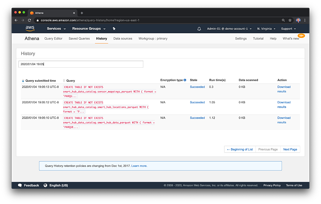
We can view any Athena SQL query from the Athena Console’s History tab. Clicking on a query (in pink) will copy it to the Query Editor tab and execute it. Below, we see the three SQL statements executed by the Lamba functions.
AWS Glue ETL Job for XML
If you recall, the electrical rate data is in XML format. The Lambda functions we just executed, converted the CSV and JSON data to Parquet using Athena. Currently, unlike CSV, JSON, ORC, Parquet, and Avro, Athena does not support the older XML data format. For the XML data files, we will use an AWS Glue ETL Job to convert the XML data to Parquet. The Glue ETL Job is written in Python and uses Apache Spark, along with several AWS Glue PySpark extensions. For this job, I used an existing script created in the Glue ETL Jobs Console as a base, then modified the script to meet my needs.
This file contains bidirectional Unicode text that may be interpreted or compiled differently than what appears below. To review, open the file in an editor that reveals hidden Unicode characters.
Learn more about bidirectional Unicode characters
| import sys | |
| from awsglue.transforms import * | |
| from awsglue.utils import getResolvedOptions | |
| from pyspark.context import SparkContext | |
| from awsglue.context import GlueContext | |
| from awsglue.job import Job | |
| args = getResolvedOptions(sys.argv, [ | |
| 'JOB_NAME', | |
| 's3_output_path', | |
| 'source_glue_database', | |
| 'source_glue_table' | |
| ]) | |
| s3_output_path = args['s3_output_path'] | |
| source_glue_database = args['source_glue_database'] | |
| source_glue_table = args['source_glue_table'] | |
| sc = SparkContext() | |
| glueContext = GlueContext(sc) | |
| spark = glueContext.spark_session | |
| job = Job(glueContext) | |
| job.init(args['JOB_NAME'], args) | |
| datasource0 = glueContext. \ | |
| create_dynamic_frame. \ | |
| from_catalog(database=source_glue_database, | |
| table_name=source_glue_table, | |
| transformation_ctx="datasource0") | |
| applymapping1 = ApplyMapping.apply( | |
| frame=datasource0, | |
| mappings=[("from", "string", "from", "string"), | |
| ("to", "string", "to", "string"), | |
| ("type", "string", "type", "string"), | |
| ("rate", "double", "rate", "double"), | |
| ("year", "int", "year", "int"), | |
| ("month", "int", "month", "int"), | |
| ("state", "string", "state", "string")], | |
| transformation_ctx="applymapping1") | |
| resolvechoice2 = ResolveChoice.apply( | |
| frame=applymapping1, | |
| choice="make_struct", | |
| transformation_ctx="resolvechoice2") | |
| dropnullfields3 = DropNullFields.apply( | |
| frame=resolvechoice2, | |
| transformation_ctx="dropnullfields3") | |
| datasink4 = glueContext.write_dynamic_frame.from_options( | |
| frame=dropnullfields3, | |
| connection_type="s3", | |
| connection_options={ | |
| "path": s3_output_path, | |
| "partitionKeys": ["state"] | |
| }, | |
| format="parquet", | |
| transformation_ctx="datasink4") | |
| job.commit() |
The three Python command-line arguments the script expects (lines 10–12, above) are defined in the CloudFormation template, smart-hub-athena-glue.yml. Below, we see them on lines 10–12 of the CloudFormation snippet. They are injected automatically when the job is run and can be overridden from the command line when starting the job.
This file contains bidirectional Unicode text that may be interpreted or compiled differently than what appears below. To review, open the file in an editor that reveals hidden Unicode characters.
Learn more about bidirectional Unicode characters
| GlueJobRatesToParquet: | |
| Type: AWS::Glue::Job | |
| Properties: | |
| GlueVersion: 1.0 | |
| Command: | |
| Name: glueetl | |
| PythonVersion: 3 | |
| ScriptLocation: !Sub "s3://${ScriptBucketName}/glue_scripts/rates_xml_to_parquet.py" | |
| DefaultArguments: { | |
| "–s3_output_path": !Sub "s3://${DataBucketName}/electricity_rates_parquet", | |
| "–source_glue_database": !Ref GlueDatabase, | |
| "–source_glue_table": "electricity_rates_xml", | |
| "–job-bookmark-option": "job-bookmark-enable", | |
| "–enable-spark-ui": "true", | |
| "–spark-event-logs-path": !Sub "s3://${LogBucketName}/glue-etl-jobs/" | |
| } | |
| Description: "Convert electrical rates XML data to Parquet" | |
| ExecutionProperty: | |
| MaxConcurrentRuns: 2 | |
| MaxRetries: 0 | |
| Name: rates-xml-to-parquet | |
| Role: !GetAtt "CrawlerRole.Arn" | |
| DependsOn: | |
| – CrawlerRole | |
| – GlueDatabase | |
| – DataBucket | |
| – ScriptBucket | |
| – LogBucket |
First, copy the Glue ETL Job Python script to the SCRIPT_BUCKET S3 bucket.
This file contains bidirectional Unicode text that may be interpreted or compiled differently than what appears below. To review, open the file in an editor that reveals hidden Unicode characters.
Learn more about bidirectional Unicode characters
| aws s3 cp glue-scripts/rates_xml_to_parquet.py \ | |
| s3://${SCRIPT_BUCKET}/glue_scripts/ |
Next, start the Glue ETL Job (part of step 2a in workflow diagram). Although the conversion is a relatively simple set of tasks, the creation of the Apache Spark environment, to execute the tasks, will take several minutes. Whereas the Glue Crawlers took about 2 minutes on average, the Glue ETL Job could take 10–15 minutes in my experience. The actual execution time only takes about 1–2 minutes of the 10–15 minutes to complete. In my opinion, waiting up to 15 minutes is too long to be viable for ad-hoc jobs against smaller datasets; Glue ETL Jobs are definitely targeted for big data.
This file contains bidirectional Unicode text that may be interpreted or compiled differently than what appears below. To review, open the file in an editor that reveals hidden Unicode characters.
Learn more about bidirectional Unicode characters
| aws glue start-job-run –job-name rates-xml-to-parquet |
To check on the status of the job, use the Glue ETL Jobs Console, or use the AWS CLI.
This file contains bidirectional Unicode text that may be interpreted or compiled differently than what appears below. To review, open the file in an editor that reveals hidden Unicode characters.
Learn more about bidirectional Unicode characters
| # get status of most recent job (the one that is running) | |
| aws glue get-job-run \ | |
| –job-name rates-xml-to-parquet \ | |
| –run-id "$(aws glue get-job-runs \ | |
| –job-name rates-xml-to-parquet \ | |
| | jq -r '.JobRuns[0].Id')" |
When complete, you should see results similar to the following. Note the ‘JobRunState’ is ‘SUCCEEDED.’ This particular job ran for a total of 14.92 minutes, while the actual execution time was 2.25 minutes.
This file contains bidirectional Unicode text that may be interpreted or compiled differently than what appears below. To review, open the file in an editor that reveals hidden Unicode characters.
Learn more about bidirectional Unicode characters
| { | |
| "JobRun": { | |
| "Id": "jr_f7186b26bf042ea7773ad08704d012d05299f080e7ac9b696ca8dd575f79506b", | |
| "Attempt": 0, | |
| "JobName": "rates-xml-to-parquet", | |
| "StartedOn": 1578022390.301, | |
| "LastModifiedOn": 1578023285.632, | |
| "CompletedOn": 1578023285.632, | |
| "JobRunState": "SUCCEEDED", | |
| "PredecessorRuns": [], | |
| "AllocatedCapacity": 10, | |
| "ExecutionTime": 135, | |
| "Timeout": 2880, | |
| "MaxCapacity": 10.0, | |
| "LogGroupName": "/aws-glue/jobs", | |
| "GlueVersion": "1.0" | |
| } | |
| } |
The job’s progress and the results are also visible in the AWS Glue Console’s ETL Jobs tab.

Detailed Apache Spark logs are also available in CloudWatch Management Console, which is accessible directly from the Logs link in the AWS Glue Console’s ETL Jobs tab.

The last step in the Data Transformation stage is to convert catalog the Parquet-format electrical rates data, created with the previous Glue ETL Job, using yet another Glue Crawler (part of step 2b in workflow diagram). Start the following Glue Crawler to catalog the Parquet-format electrical rates data.
This file contains bidirectional Unicode text that may be interpreted or compiled differently than what appears below. To review, open the file in an editor that reveals hidden Unicode characters.
Learn more about bidirectional Unicode characters
| aws glue start-crawler –name smart-hub-rates-parquet |
This concludes the Data Transformation stage. The raw and transformed data is in the data lake, and the following nine tables should exist in the Glue Data Catalog.
This file contains bidirectional Unicode text that may be interpreted or compiled differently than what appears below. To review, open the file in an editor that reveals hidden Unicode characters.
Learn more about bidirectional Unicode characters
| electricity_rates_parquet | |
| electricity_rates_xml | |
| etl_tmp_output_parquet | |
| sensor_mappings_json | |
| sensor_mappings_parquet | |
| smart_hub_data_json | |
| smart_hub_data_parquet | |
| smart_hub_locations_csv | |
| smart_hub_locations_parquet |
If we examine the tables, we should observe the data partitions we used to organize the data files in the Amazon S3-based data lake are contained in the table metadata. Below, we see the four partitions, based on state, of the Parquet-format locations data.

Data Enrichment
To begin the Data Enrichment stage, we will invoke the AWS Lambda, athena-complex-etl-query/index.py. This Lambda accepts input parameters (lines 28–30, below), passed in the Lambda handler’s event parameter. The arguments include the Smart Hub ID, the start date for the data requested, and the end date for the data requested. The scenario for the demonstration is that a customer with the location id value, using the electrical provider’s application, has requested data for a particular range of days (start date and end date), to visualize and analyze.
The Lambda executes a series of Athena INSERT INTO SQL statements, one statement for each of the possible Smart Hub connected electrical sensors, s_01 through s_10, for which there are values in the Smart Hub electrical usage data. Amazon just released the Amazon Athena INSERT INTO a table using the results of a SELECT query capability in September 2019, an essential addition to Athena. New Athena features are listed in the release notes.
Here, the SELECT query is actually a series of chained subqueries, using Presto SQL’s WITH clause capability. The queries join the Parquet-format Smart Hub electrical usage data sources in the S3-based data lake, with the other three Parquet-format, S3-based data sources: sensor mappings, locations, and electrical rates. The Parquet-format data is written as individual files to S3 and inserted into the existing ‘etl_tmp_output_parquet’ Glue Data Catalog database table. Compared to traditional relational database-based queries, the capabilities of Glue and Athena to enable complex SQL queries across multiple semi-structured data files, stored in S3, is truly amazing!
The capabilities of Glue and Athena to enable complex SQL queries across multiple semi-structured data files, stored in S3, is truly amazing!
Below, we see the SQL statement starting on line 43.
This file contains bidirectional Unicode text that may be interpreted or compiled differently than what appears below. To review, open the file in an editor that reveals hidden Unicode characters.
Learn more about bidirectional Unicode characters
| import boto3 | |
| import os | |
| import logging | |
| import json | |
| from typing import Dict | |
| # environment variables | |
| data_catalog = os.getenv('DATA_CATALOG') | |
| data_bucket = os.getenv('DATA_BUCKET') | |
| # variables | |
| output_directory = 'etl_tmp_output_parquet' | |
| # uses list comprehension to generate the equivalent of: | |
| # ['s_01', 's_02', …, 's_09', 's_10'] | |
| sensors = [f's_{i:02d}' for i in range(1, 11)] | |
| # logging | |
| logger = logging.getLogger() | |
| logger.setLevel(logging.INFO) | |
| # athena client | |
| athena_client = boto3.client('athena') | |
| def handler(event, context): | |
| args = { | |
| "loc_id": event['loc_id'], | |
| "date_from": event['date_from'], | |
| "date_to": event['date_to'] | |
| } | |
| athena_query(args) | |
| return { | |
| 'statusCode': 200, | |
| 'body': json.dumps("function 'athena-complex-etl-query' complete") | |
| } | |
| def athena_query(args: Dict[str, str]): | |
| for sensor in sensors: | |
| query = \ | |
| "INSERT INTO " + data_catalog + "." + output_directory + " " \ | |
| "WITH " \ | |
| " t1 AS " \ | |
| " (SELECT d.loc_id, d.ts, d.data." + sensor + " AS kwh, l.state, l.tz " \ | |
| " FROM smart_hub_data_catalog.smart_hub_data_parquet d " \ | |
| " LEFT OUTER JOIN smart_hub_data_catalog.smart_hub_locations_parquet l " \ | |
| " ON d.loc_id = l.hash " \ | |
| " WHERE d.loc_id = '" + args['loc_id'] + "' " \ | |
| " AND d.dt BETWEEN cast('" + args['date_from'] + \ | |
| "' AS date) AND cast('" + args['date_to'] + "' AS date)), " \ | |
| " t2 AS " \ | |
| " (SELECT at_timezone(from_unixtime(t1.ts, 'UTC'), t1.tz) AS ts, " \ | |
| " date_format(at_timezone(from_unixtime(t1.ts, 'UTC'), t1.tz), '%H') AS rate_period, " \ | |
| " m.description AS device, m.location, t1.loc_id, t1.state, t1.tz, t1.kwh " \ | |
| " FROM t1 LEFT OUTER JOIN smart_hub_data_catalog.sensor_mappings_parquet m " \ | |
| " ON t1.loc_id = m.loc_id " \ | |
| " WHERE t1.loc_id = '" + args['loc_id'] + "' " \ | |
| " AND m.state = t1.state " \ | |
| " AND m.description = (SELECT m2.description " \ | |
| " FROM smart_hub_data_catalog.sensor_mappings_parquet m2 " \ | |
| " WHERE m2.loc_id = '" + args['loc_id'] + "' AND m2.id = '" + sensor + "')), " \ | |
| " t3 AS " \ | |
| " (SELECT substr(r.to, 1, 2) AS rate_period, r.type, r.rate, r.year, r.month, r.state " \ | |
| " FROM smart_hub_data_catalog.electricity_rates_parquet r " \ | |
| " WHERE r.year BETWEEN cast(date_format(cast('" + args['date_from'] + \ | |
| "' AS date), '%Y') AS integer) AND cast(date_format(cast('" + args['date_to'] + \ | |
| "' AS date), '%Y') AS integer)) " \ | |
| "SELECT replace(cast(t2.ts AS VARCHAR), concat(' ', t2.tz), '') AS ts, " \ | |
| " t2.device, t2.location, t3.type, t2.kwh, t3.rate AS cents_per_kwh, " \ | |
| " round(t2.kwh * t3.rate, 4) AS cost, t2.state, t2.loc_id " \ | |
| "FROM t2 LEFT OUTER JOIN t3 " \ | |
| " ON t2.rate_period = t3.rate_period " \ | |
| "WHERE t3.state = t2.state " \ | |
| "ORDER BY t2.ts, t2.device;" | |
| logger.info(query) | |
| response = athena_client.start_query_execution( | |
| QueryString=query, | |
| QueryExecutionContext={ | |
| 'Database': data_catalog | |
| }, | |
| ResultConfiguration={ | |
| 'OutputLocation': 's3://' + data_bucket + '/tmp/' + output_directory | |
| }, | |
| WorkGroup='primary' | |
| ) | |
| logger.info(response) |
Below, is an example of one of the final queries, for the s_10 sensor, as executed by Athena. All the input parameter values, Python variables, and environment variables have been resolved into the query.
This file contains bidirectional Unicode text that may be interpreted or compiled differently than what appears below. To review, open the file in an editor that reveals hidden Unicode characters.
Learn more about bidirectional Unicode characters
| INSERT INTO smart_hub_data_catalog.etl_tmp_output_parquet | |
| WITH t1 AS (SELECT d.loc_id, d.ts, d.data.s_10 AS kwh, l.state, l.tz | |
| FROM smart_hub_data_catalog.smart_hub_data_parquet d | |
| LEFT OUTER JOIN smart_hub_data_catalog.smart_hub_locations_parquet l ON d.loc_id = l.hash | |
| WHERE d.loc_id = 'b6a8d42425fde548' | |
| AND d.dt BETWEEN cast('2019-12-21' AS date) AND cast('2019-12-22' AS date)), | |
| t2 AS (SELECT at_timezone(from_unixtime(t1.ts, 'UTC'), t1.tz) AS ts, | |
| date_format(at_timezone(from_unixtime(t1.ts, 'UTC'), t1.tz), '%H') AS rate_period, | |
| m.description AS device, | |
| m.location, | |
| t1.loc_id, | |
| t1.state, | |
| t1.tz, | |
| t1.kwh | |
| FROM t1 | |
| LEFT OUTER JOIN smart_hub_data_catalog.sensor_mappings_parquet m ON t1.loc_id = m.loc_id | |
| WHERE t1.loc_id = 'b6a8d42425fde548' | |
| AND m.state = t1.state | |
| AND m.description = (SELECT m2.description | |
| FROM smart_hub_data_catalog.sensor_mappings_parquet m2 | |
| WHERE m2.loc_id = 'b6a8d42425fde548' | |
| AND m2.id = 's_10')), | |
| t3 AS (SELECT substr(r.to, 1, 2) AS rate_period, r.type, r.rate, r.year, r.month, r.state | |
| FROM smart_hub_data_catalog.electricity_rates_parquet r | |
| WHERE r.year BETWEEN cast(date_format(cast('2019-12-21' AS date), '%Y') AS integer) | |
| AND cast(date_format(cast('2019-12-22' AS date), '%Y') AS integer)) | |
| SELECT replace(cast(t2.ts AS VARCHAR), concat(' ', t2.tz), '') AS ts, | |
| t2.device, | |
| t2.location, | |
| t3.type, | |
| t2.kwh, | |
| t3.rate AS cents_per_kwh, | |
| round(t2.kwh * t3.rate, 4) AS cost, | |
| t2.state, | |
| t2.loc_id | |
| FROM t2 | |
| LEFT OUTER JOIN t3 ON t2.rate_period = t3.rate_period | |
| WHERE t3.state = t2.state | |
| ORDER BY t2.ts, t2.device; |
Along with enriching the data, the query performs additional data transformation using the other data sources. For example, the Unix timestamp is converted to a localized timestamp containing the date and time, according to the customer’s location (line 7, above). Transforming dates and times is a frequent, often painful, data analysis task. Another example of data enrichment is the augmentation of the data with a new, computed column. The column’s values are calculated using the values of two other columns (line 33, above).
Invoke the Lambda with the following three parameters in the payload (step 3a in workflow diagram).
This file contains bidirectional Unicode text that may be interpreted or compiled differently than what appears below. To review, open the file in an editor that reveals hidden Unicode characters.
Learn more about bidirectional Unicode characters
| aws lambda invoke \ | |
| –function-name athena-complex-etl-query \ | |
| –payload "{ \"loc_id\": \"b6a8d42425fde548\", | |
| \"date_from\": \"2019-12-21\", \"date_to\": \"2019-12-22\"}" \ | |
| response.json |
The ten INSERT INTO SQL statement’s result statuses (one per device sensor) are visible from the Athena Console’s History tab.

Each Athena query execution saves that query’s results to the S3-based data lake as individual, uncompressed Parquet-format data files. The data is partitioned in the Amazon S3-based data lake by the Smart Meter location ID (e.g., ‘loc_id=b6a8d42425fde548’).
Below is a snippet of the enriched data for a customer’s clothes washer (sensor ‘s_04’). Note the timestamp is now an actual date and time in the local timezone of the customer (e.g., ‘2019-12-21 20:10:00.000’). The sensor ID (‘s_04’) is replaced with the actual device name (‘Clothes Washer’). The location of the device (‘Basement’) and the type of electrical usage period (e.g. ‘peak’ or ‘partial-peak’) has been added. Finally, the cost column has been computed.
This file contains bidirectional Unicode text that may be interpreted or compiled differently than what appears below. To review, open the file in an editor that reveals hidden Unicode characters.
Learn more about bidirectional Unicode characters
| ts | device | location | type | kwh | cents_per_kwh | cost | state | loc_id | |
|---|---|---|---|---|---|---|---|---|---|
| 2019-12-21 19:40:00.000 | Clothes Washer | Basement | peak | 0.0 | 12.623 | 0.0 | or | b6a8d42425fde548 | |
| 2019-12-21 19:45:00.000 | Clothes Washer | Basement | peak | 0.0 | 12.623 | 0.0 | or | b6a8d42425fde548 | |
| 2019-12-21 19:50:00.000 | Clothes Washer | Basement | peak | 0.1501 | 12.623 | 1.8947 | or | b6a8d42425fde548 | |
| 2019-12-21 19:55:00.000 | Clothes Washer | Basement | peak | 0.1497 | 12.623 | 1.8897 | or | b6a8d42425fde548 | |
| 2019-12-21 20:00:00.000 | Clothes Washer | Basement | partial-peak | 0.1501 | 7.232 | 1.0855 | or | b6a8d42425fde548 | |
| 2019-12-21 20:05:00.000 | Clothes Washer | Basement | partial-peak | 0.2248 | 7.232 | 1.6258 | or | b6a8d42425fde548 | |
| 2019-12-21 20:10:00.000 | Clothes Washer | Basement | partial-peak | 0.2247 | 7.232 | 1.625 | or | b6a8d42425fde548 | |
| 2019-12-21 20:15:00.000 | Clothes Washer | Basement | partial-peak | 0.2248 | 7.232 | 1.6258 | or | b6a8d42425fde548 | |
| 2019-12-21 20:20:00.000 | Clothes Washer | Basement | partial-peak | 0.2253 | 7.232 | 1.6294 | or | b6a8d42425fde548 | |
| 2019-12-21 20:25:00.000 | Clothes Washer | Basement | partial-peak | 0.151 | 7.232 | 1.092 | or | b6a8d42425fde548 |
To transform the enriched CSV-format data to Parquet-format, we need to catalog the CSV-format results using another Crawler, first (step 3d in workflow diagram).
This file contains bidirectional Unicode text that may be interpreted or compiled differently than what appears below. To review, open the file in an editor that reveals hidden Unicode characters.
Learn more about bidirectional Unicode characters
| aws glue start-crawler –name smart-hub-etl-tmp-output-parquet |
Optimizing Enriched Data
The previous step created enriched Parquet-format data. However, this data is not as optimized for query efficiency as it should be. Using the Athena INSERT INTO WITH SQL statement, allowed the data to be partitioned. However, the method does not allow the Parquet data to be easily combined into larger files and compressed. To perform both these optimizations, we will use one last Lambda, athena-parquet-to-parquet-elt-data/index.py. The Lambda will create a new location in the Amazon S3-based data lake, containing all the enriched data, in a single file and compressed using Snappy compression.
This file contains bidirectional Unicode text that may be interpreted or compiled differently than what appears below. To review, open the file in an editor that reveals hidden Unicode characters.
Learn more about bidirectional Unicode characters
| aws lambda invoke \ | |
| –function-name athena-parquet-to-parquet-elt-data \ | |
| response.json |
The resulting Parquet file is visible in the S3 Management Console.

The final step in the Data Enrichment stage is to catalog the optimized Parquet-format enriched ETL data. To catalog the data, run the following Glue Crawler (step 3i in workflow diagram
This file contains bidirectional Unicode text that may be interpreted or compiled differently than what appears below. To review, open the file in an editor that reveals hidden Unicode characters.
Learn more about bidirectional Unicode characters
| aws glue start-crawler –name smart-hub-etl-output-parquet |
Final Data Lake and Data Catalog
We should now have the following ten top-level folders of partitioned data in the S3-based data lake. The ‘tmp’ folder may be ignored.
This file contains bidirectional Unicode text that may be interpreted or compiled differently than what appears below. To review, open the file in an editor that reveals hidden Unicode characters.
Learn more about bidirectional Unicode characters
| aws s3 ls s3://${DATA_BUCKET}/ |
This file contains bidirectional Unicode text that may be interpreted or compiled differently than what appears below. To review, open the file in an editor that reveals hidden Unicode characters.
Learn more about bidirectional Unicode characters
| PRE electricity_rates_parquet/ | |
| PRE electricity_rates_xml/ | |
| PRE etl_output_parquet/ | |
| PRE etl_tmp_output_parquet/ | |
| PRE sensor_mappings_json/ | |
| PRE sensor_mappings_parquet/ | |
| PRE smart_hub_data_json/ | |
| PRE smart_hub_data_parquet/ | |
| PRE smart_hub_locations_csv/ | |
| PRE smart_hub_locations_parquet/ |
Similarly, we should now have the following ten corresponding tables in the Glue Data Catalog. Use the AWS Glue Console to confirm the tables exist.

Alternately, use the following AWS CLI / jq command to list the table names.
This file contains bidirectional Unicode text that may be interpreted or compiled differently than what appears below. To review, open the file in an editor that reveals hidden Unicode characters.
Learn more about bidirectional Unicode characters
| aws glue get-tables \ | |
| –database-name smart_hub_data_catalog \ | |
| | jq -r '.TableList[].Name' |
This file contains bidirectional Unicode text that may be interpreted or compiled differently than what appears below. To review, open the file in an editor that reveals hidden Unicode characters.
Learn more about bidirectional Unicode characters
| electricity_rates_parquet | |
| electricity_rates_xml | |
| etl_output_parquet | |
| etl_tmp_output_parquet | |
| sensor_mappings_json | |
| sensor_mappings_parquet | |
| smart_hub_data_json | |
| smart_hub_data_parquet | |
| smart_hub_locations_csv | |
| smart_hub_locations_parquet |
‘Unknown’ Bug
You may have noticed the four tables created with the AWS Lambda functions, using the CTAS SQL statement, erroneously have the ‘Classification’ of ‘Unknown’ as opposed to ‘parquet’. I am not sure why, I believe it is a possible bug with the CTAS feature. It seems to have no adverse impact on the table’s functionality. However, to fix the issue, run the following set of commands. This aws glue update-table hack will switch the table’s ‘Classification’ to ‘parquet’.
This file contains bidirectional Unicode text that may be interpreted or compiled differently than what appears below. To review, open the file in an editor that reveals hidden Unicode characters.
Learn more about bidirectional Unicode characters
| database=smart_hub_data_catalog | |
| tables=(smart_hub_locations_parquet sensor_mappings_parquet smart_hub_data_parquet etl_output_parquet) | |
| for table in ${tables}; do | |
| fixed_table=$(aws glue get-table \ | |
| –database-name "${database}" \ | |
| –name "${table}" \ | |
| | jq '.Table.Parameters.classification = "parquet" | del(.Table.DatabaseName) | del(.Table.CreateTime) | del(.Table.UpdateTime) | del(.Table.CreatedBy) | del(.Table.IsRegisteredWithLakeFormation)') | |
| fixed_table=$(echo ${fixed_table} | jq .Table) | |
| aws glue update-table \ | |
| –database-name "${database}" \ | |
| –table-input "${fixed_table}" | |
| echo "table '${table}' classification changed to 'parquet'" | |
| done |
The results of the fix may be seen from the AWS Glue Console. All ten tables are now classified correctly.

Explore the Data
Before starting to visualize and analyze the data with Amazon QuickSight, try executing a few Athena queries against the tables in the Glue Data Catalog database, using the Athena Query Editor. Working in the Editor is the best way to understand the data, learn Athena, and debug SQL statements and queries. The Athena Query Editor has convenient developer features like SQL auto-complete and query formatting capabilities.
Be mindful when writing queries and searching the Internet for SQL references, the Athena query engine is based on Presto 0.172. The current version of Presto, 0.229, is more than 50 releases ahead of the current Athena version. Both Athena and Presto functionality has changed and diverged. There are additional considerations and limitations for SQL queries in Athena to be aware of.
Here are a few simple, ad-hoc queries to run in the Athena Query Editor.
This file contains bidirectional Unicode text that may be interpreted or compiled differently than what appears below. To review, open the file in an editor that reveals hidden Unicode characters.
Learn more about bidirectional Unicode characters
| — preview the final etl data | |
| SELECT * | |
| FROM smart_hub_data_catalog.etl_output_parquet | |
| LIMIT 10; | |
| — total cost in $'s for each device, at location 'b6a8d42425fde548' | |
| — from high to low, on December 21, 2019 | |
| SELECT device, | |
| concat('$', cast(cast(sum(cost) / 100 AS decimal(10, 2)) AS varchar)) AS total_cost | |
| FROM smart_hub_data_catalog.etl_tmp_output_parquet | |
| WHERE loc_id = 'b6a8d42425fde548' | |
| AND date (cast(ts AS timestamp)) = date '2019-12-21' | |
| GROUP BY device | |
| ORDER BY total_cost DESC; | |
| — count of smart hub residential locations in Oregon and California, | |
| — grouped by zip code, sorted by count | |
| SELECT DISTINCT postcode, upper(state), count(postcode) AS smart_hub_count | |
| FROM smart_hub_data_catalog.smart_hub_locations_parquet | |
| WHERE state IN ('or', 'ca') | |
| AND length(cast(postcode AS varchar)) >= 5 | |
| GROUP BY state, postcode | |
| ORDER BY smart_hub_count DESC, postcode; | |
| — electrical usage for the clothes washer | |
| — over a 30-minute period, on December 21, 2019 | |
| SELECT ts, device, location, type, cost | |
| FROM smart_hub_data_catalog.etl_tmp_output_parquet | |
| WHERE loc_id = 'b6a8d42425fde548' | |
| AND device = 'Clothes Washer' | |
| AND cast(ts AS timestamp) | |
| BETWEEN timestamp '2019-12-21 08:45:00' | |
| AND timestamp '2019-12-21 09:15:00' | |
| ORDER BY ts; |
Cleaning Up
You may choose to save the AWS resources created in part one of this demonstration, to be used in part two. Since you are not actively running queries against the data, ongoing AWS costs will be minimal. If you eventually choose to clean up the AWS resources created in part one of this demonstration, execute the following AWS CLI commands. To avoid failures, make sure each command completes before running the subsequent command. You will need to confirm the CloudFormation stacks are deleted using the AWS CloudFormation Console or the AWS CLI. These commands will not remove Amazon QuickSight data sets, analyses, and dashboards created in part two. However, deleting the AWS Glue Data Catalog and the underlying data sources will impact the ability to visualize the data in QuickSight.
This file contains bidirectional Unicode text that may be interpreted or compiled differently than what appears below. To review, open the file in an editor that reveals hidden Unicode characters.
Learn more about bidirectional Unicode characters
| # delete s3 contents first | |
| aws s3 rm s3://${DATA_BUCKET} –recursive | |
| aws s3 rm s3://${SCRIPT_BUCKET} –recursive | |
| aws s3 rm s3://${LOG_BUCKET} –recursive | |
| # then, delete lambda cfn stack | |
| aws cloudformation delete-stack –stack-name smart-hub-lambda-stack | |
| # finally, delete athena-glue-s3 stack | |
| aws cloudformation delete-stack –stack-name smart-hub-athena-glue-stack |
Part Two
In part one, starting with raw, semi-structured data in multiple formats, we learned how to ingest, transform, and enrich that data using Amazon S3, AWS Glue, Amazon Athena, and AWS Lambda. We built an S3-based data lake and learned how AWS leverages open-source technologies, including Presto, Apache Hive, and Apache Parquet. In part two of this post, we will use the transformed and enriched datasets, stored in the data lake, to create compelling visualizations using Amazon QuickSight.
All opinions expressed in this post are my own and not necessarily the views of my current or past employers or their clients.
Using the WCF Web HTTP Programming Model with Entity Framework 5
Posted by Gary A. Stafford in .NET Development, Client-Side Development, Software Development on December 12, 2012
Build a IIS-hosted WCF Service using the WCF Web HTTP Programming Model. Use basic HTTP Methods with the WCF Service to perform CRUD operations on a SQL Server database using a Data Access Layer, built with Entity Framework 5 and the Database First Development Model.
You can download a complete copy of this Post’s source code from DropBox.
Introduction
In the two previous Posts, we used the new Entity Framework 5 to create a Data Access Layer, using both the Code First and Database First Development Models. In this Post, we will create a Windows Communication Foundation (WCF) Service. The service will sit between the client application and our previous Post’s Data Access Layer (DAL), built with an ADO.NET Entity Data Model (EDM). Using the WCF Web HTTP Programming Model, we will expose the WCF Service’s operations to a non-SOAP endpoint, and call them using HTTP Methods.
Why use the WCF Web HTTP Programming Model? WCF is a well-established, reliable, secure, enterprise technology. Many large, as well as small, organizations use WCF to build service-oriented applications. However, as communications become increasingly Internet-enabled and mobile, the WCF Web HTTP Programming Model allows us to add the use of simple HTTP methods, such as POST, GET, DELETE, and PUT, to existing WCF services. Adding a web endpoint to an existing WCF service extends its reach to modern end-user platforms with minimal effort. Lastly, using the WCF Web HTTP Programming Model allows us to move toward the increasingly popular RESTful Web Service Model, so many organizations are finally starting to embrace in the enterprise.
Creating the WCF Service
The major steps involved in this example are as follows:
- Create a new WCF Service Application Project;
- Add the Entity Framework package via NuGet;
- Add a Reference the previous Post’s DAL project;
- Add a Connection String to the project’s configuration;
- Create the WCF Service Contract;
- Create the operations the service will expose via a web endpoint;
- Configure the service’s behaviors, binding, and web endpoint;
- Publish the WCF Service to IIS using VS2012’s Web Project Publishing Tool;
- Test the service’s operations with Fiddler.
The WCF Service Application Project

Solution Explorer View of New Solution for Reference
Start by creating a new Visual Studio 2012 WCF Service Application Project, named ‘HealthTracker.WcfService’. Add it to a new Solution, named ‘HealthTracker’. The WCF Service Application Project type is specifically designed to be hosted by Microsoft’s Internet Information Services (IIS).
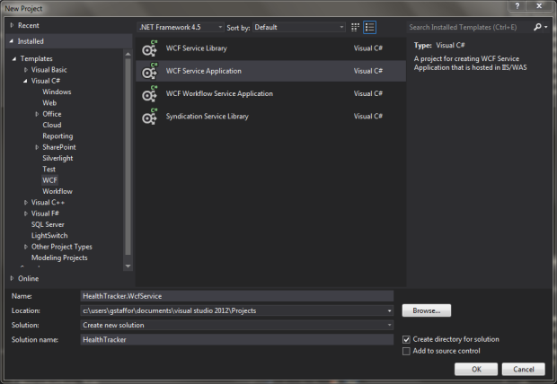
Create New WCF Service Application Project
Once the Project and Solution are created, install Entity Framework (‘System.Data.Entity’) into the Solution by right-clicking on the Solution and selecting ‘Manage NuGet Packages for Solution…’ Install the ‘EntityFramework’ package. If you haven’t discovered the power of NuGet for Visual Studio, check out their site.

Manage NuGet Packages – Add Entity Framework to Solution
Next, add a Reference in the new Project, to the previous ‘HealthTracker.DataAccess.DbFirst’ Project. When the WCF Service Application Project is built, a copy of the ‘HealthTracker.DataAccess.DbFirst.dll’ assembly will be placed into the ‘bin’ folder of the ‘HealthTracker.WcfService’ Project.

Add a Reference to Previous EF5 Database First Project
Next, copy the connection string from the previous project’s ‘App.Config file’ and paste into the new WCF Service Application Project’s ‘Web.config’ file. The connection is required by the ‘HealthTracker.DataAccess.DbFirst.dll’ assembly. The connection string should look similar to the below code.
<connectionStrings>
<add name="HealthTrackerEntities" connectionString="metadata=res://*/HealthTracker.csdl|res://*/HealthTracker.ssdl|res://*/HealthTracker.msl;provider=System.Data.SqlClient;provider connection string="data source=[Your_Server]\[Your_SQL_Instance];initial catalog=HealthTracker;persist security info=True;user id=DemoLogin;password=[Your_Password];MultipleActiveResultSets=True;App=EntityFramework"" providerName="System.Data.EntityClient" />
</connectionStrings>
The WCF Service
Delete the default ‘Service.svc’ and ‘IService.cs’ created by the Project Template. You can also delete the default ‘App_Data’ folder. Add a new WCF Service, named ‘HealthTrackerWcfService.svc’. Adding a new service creates both the WCF Service file (.svc), as well as a WCF Service Contract file (.cs), an Interface, named ‘IHealthTrackerWcfService.cs’. The ‘HealthTrackerWcfService’ class implements the ‘IHealthTrackerWcfService’ Interface class (‘public class HealthTrackerWcfService : IHealthTrackerWcfService’).

Add New WCF Service to Project
The WCF Service file contains public methods, called service operations, which the service will expose through a web endpoint. The second file, an Interface class, is referred to as the Service Contract. The Service Contract contains the method signatures of all the operations the service’s web endpoint expose. The Service Contract contains attributes, part of the ‘System.ServiceModel’ and ‘System.ServiceModel.Web’ Namespaces, describing how the service and its operation will be exposed. To create the Service Contract, replace the default code in the file, ‘IHealthTrackerWcfService.cs’, with the following code.
using System.Collections.Generic;
using System.ServiceModel;
using System.ServiceModel.Web;
using HealthTracker.DataAccess.DbFirst;

namespace HealthTracker.WcfService
{
    [ServiceContract]
    public interface IHealthTrackerWcfService
    {
        [OperationContract]
        [WebInvoke(UriTemplate = "GetPersonId?name={personName}",
            Method = "GET")]
        int GetPersonId(string personName);

        [OperationContract]
        [WebInvoke(UriTemplate = "GetPeople",
            Method = "GET")]
        List<Person> GetPeople();

        [OperationContract]
        [WebInvoke(UriTemplate = "GetPersonSummaryStoredProc?id={personId}",
            Method = "GET")]
        List<GetPersonSummary_Result> GetPersonSummaryStoredProc(int personId);

        [OperationContract]
        [WebInvoke(UriTemplate = "InsertPerson",
            Method = "POST")]
        bool InsertPerson(Person person);

        [OperationContract]
        [WebInvoke(UriTemplate = "UpdatePerson",
            Method = "PUT")]
        bool UpdatePerson(Person person);

        [OperationContract]
        [WebInvoke(UriTemplate = "DeletePerson?id={personId}",
            Method = "DELETE")]
        bool DeletePerson(int personId);

        [OperationContract]
        [WebInvoke(UriTemplate = "UpdateOrInsertHydration?id={personId}",
            Method = "POST")]
        bool UpdateOrInsertHydration(int personId);

        [OperationContract]
        [WebInvoke(UriTemplate = "InsertActivity",
            Method = "POST")]
        bool InsertActivity(Activity activity);

        [OperationContract]
        [WebInvoke(UriTemplate = "DeleteActivity?id={activityId}",
            Method = "DELETE")]
        bool DeleteActivity(int activityId);

        [OperationContract]
        [WebInvoke(UriTemplate = "GetActivities?id={personId}",
            Method = "GET")]
        List<ActivityDetail> GetActivities(int personId);

        [OperationContract]
        [WebInvoke(UriTemplate = "InsertMeal",
            Method = "POST")]
        bool InsertMeal(Meal meal);

        [OperationContract]
        [WebInvoke(UriTemplate = "DeleteMeal?id={mealId}",
            Method = "DELETE")]
        bool DeleteMeal(int mealId);

        [OperationContract]
        [WebInvoke(UriTemplate = "GetMeals?id={personId}",
            Method = "GET")]
        List<MealDetail> GetMeals(int personId);

        [OperationContract]
        [WebInvoke(UriTemplate = "GetPersonSummaryView?id={personId}",
            Method = "GET")]
        List<PersonSummaryView> GetPersonSummaryView(int personId);
    }
}
The service’s operations use a variety of HTTP Methods, including GET, POST, PUT, and DELETE. The operations take a mix of primitive data types, as well as complex objects as arguments. The operations also return the same variety of simple data types, as well as complex objects. Note the operation ‘InsertActivity’ for example. It takes a complex object, an ‘Activity’, as an argument, and returns a Boolean. All the CRUD operations dealing with inserting, updating, or deleting data return a Boolean, indicating success or failure of the operation’s execution. This makes unit testing and error handling on the client-side easier.
Next, we will create the WCF Service. Replace the existing contents of the ‘HealthTrackerWcfService.svc’ file with the following code.
using System;
using System.Collections.Generic;
using System.Diagnostics;
using System.Linq;
using System.ServiceModel;
using HealthTracker.DataAccess.DbFirst;
namespace HealthTracker.WcfService
{
[ServiceBehavior(AddressFilterMode = AddressFilterMode.Any)]
public class HealthTrackerWcfService : IHealthTrackerWcfService
{
private readonly DateTime _today = DateTime.Now.Date;
#region Service Operations
/// <summary>
/// Example of Adding a new Person.
/// </summary>
/// <param name="person">New Person Object</param>
/// <returns>True if successful</returns>
public bool InsertPerson(Person person)
{
try
{
using (var dbContext = new HealthTrackerEntities())
{
dbContext.People.Add(new DataAccess.DbFirst.Person { Name = person.Name });
dbContext.SaveChanges();
return true;
}
}
catch (Exception exception)
{
Debug.WriteLine(exception);
return false;
}
}
/// <summary>
/// Example of Updating a Person.
/// </summary>
/// <param name="person">New Person Object</param>
/// <returns>True if successful</returns>
public bool UpdatePerson(Person person)
{
try
{
using (var dbContext = new HealthTrackerEntities())
{
var personToUpdate = dbContext.People.First(p => p.PersonId == person.PersonId);
if (personToUpdate == null) return false;
personToUpdate.Name = person.Name;
dbContext.SaveChanges();
return true;
}
}
catch (Exception exception)
{
Debug.WriteLine(exception);
return false;
}
}
/// <summary>
/// Example of deleting a Person.
/// </summary>
/// <param name="personId">PersonId</param>
/// <returns>True if successful</returns>
public bool DeletePerson(int personId)
{
try
{
using (var dbContext = new HealthTrackerEntities())
{
var personToDelete = dbContext.People.First(p => p.PersonId == personId);
if (personToDelete == null) return false;
dbContext.People.Remove(personToDelete);
dbContext.SaveChanges();
return true;
}
}
catch (Exception exception)
{
Debug.WriteLine(exception);
return false;
}
}
/// <summary>
/// Example of finding a Person's Id.
/// </summary>
/// <param name="personName">Name of the Person to find</param>
/// <returns>Person's unique Id (PersonId)</returns>
public int GetPersonId(string personName)
{
try
{
using (var dbContext = new HealthTrackerEntities())
{
var personId = dbContext.People
.Where(person => person.Name == personName)
.Select(person => person.PersonId)
.First();
return personId;
}
}
catch (Exception exception)
{
Debug.WriteLine(exception);
return -1;
}
}
/// <summary>
/// Returns a list of all People.
/// </summary>
/// <returns>List of People</returns>
public List<Person> GetPeople()
{
try
{
using (var dbContext = new HealthTrackerEntities())
{
var people = (dbContext.People.Select(p => p));
var peopleList = people.Select(p => new Person
{
PersonId = p.PersonId,
Name = p.Name
}).ToList();
return peopleList;
}
}
catch (Exception exception)
{
Debug.WriteLine(exception);
return null;
}
}
/// <summary>
/// Example of adding a Meal.
/// </summary>
/// <param name="meal">New Meal Object</param>
/// <returns>True if successful</returns>
public bool InsertMeal(Meal meal)
{
try
{
using (var dbContext = new HealthTrackerEntities())
{
dbContext.Meals.Add(new DataAccess.DbFirst.Meal
{
PersonId = meal.PersonId,
Date = _today,
MealTypeId = meal.MealTypeId,
Description = meal.Description
});
dbContext.SaveChanges();
return true;
}
}
catch (Exception exception)
{
Debug.WriteLine(exception);
return false;
}
}
/// <summary>
/// Example of deleting a Meal.
/// </summary>
/// <param name="mealId">MealId</param>
/// <returns>True if successful</returns>
public bool DeleteMeal(int mealId)
{
try
{
using (var dbContext = new HealthTrackerEntities())
{
var mealToDelete = dbContext.Meals.First(m => m.MealTypeId == mealId);
if (mealToDelete == null) return false;
dbContext.Meals.Remove(mealToDelete);
dbContext.SaveChanges();
return true;
}
}
catch (Exception exception)
{
Debug.WriteLine(exception);
return false;
}
}
/// <summary>
/// Return all Meals for a Person.
/// </summary>
/// <param name="personId">PersonId</param>
/// <returns></returns>
public List<MealDetail> GetMeals(int personId)
{
try
{
using (var dbContext = new HealthTrackerEntities())
{
var meals = dbContext.Meals.Where(m => m.PersonId == personId)
.Select(m => new MealDetail
{
MealId = m.MealId,
Date = m.Date,
Type = m.MealType.Description,
Description = m.Description
}).ToList();
return meals;
}
}
catch (Exception exception)
{
Debug.WriteLine(exception);
return null;
}
}
/// <summary>
/// Example of adding an Activity.
/// </summary>
/// <param name="activity">New Activity Object</param>
/// <returns>True if successful</returns>
public bool InsertActivity(Activity activity)
{
try
{
using (var dbContext = new HealthTrackerEntities())
{
dbContext.Activities.Add(new DataAccess.DbFirst.Activity
{
PersonId = activity.PersonId,
Date = _today,
ActivityTypeId = activity.ActivityTypeId,
Notes = activity.Notes
});
dbContext.SaveChanges();
return true;
}
}
catch (Exception exception)
{
Debug.WriteLine(exception);
return false;
}
}
/// <summary>
/// Example of deleting a Activity.
/// </summary>
/// <param name="activityId">ActivityId</param>
/// <returns>True if successful</returns>
public bool DeleteActivity(int activityId)
{
try
{
using (var dbContext = new HealthTrackerEntities())
{
var activityToDelete = dbContext.Activities.First(a => a.ActivityId == activityId);
if (activityToDelete == null) return false;
dbContext.Activities.Remove(activityToDelete);
dbContext.SaveChanges();
return true;
}
}
catch (Exception exception)
{
Debug.WriteLine(exception);
return false;
}
}
/// <summary>
/// Return all Activities for a Person.
/// </summary>
/// <param name="personId">PersonId</param>
/// <returns>List of Activities</returns>
public List<ActivityDetail> GetActivities(int personId)
{
try
{
using (var dbContext = new HealthTrackerEntities())
{
var activities = dbContext.Activities.Where(a => a.PersonId == personId)
.Select(a => new ActivityDetail
{
ActivityId = a.ActivityId,
Date = a.Date,
Type = a.ActivityType.Description,
Notes = a.Notes
}).ToList();
return activities;
}
}
catch (Exception exception)
{
Debug.WriteLine(exception);
return null;
}
}
/// <summary>
/// Example of updating existing Hydration count.
/// Else adding new Hydration if it doesn't exist.
/// </summary>
/// <param name="personId">PersonId</param>
/// <returns>True if successful</returns>
public bool UpdateOrInsertHydration(int personId)
{
try
{
using (var dbContext = new HealthTrackerEntities())
{
var existingHydration = dbContext.Hydrations.First(
hydration => hydration.PersonId == personId
&& hydration.Date == _today);
if (existingHydration != null && existingHydration.HydrationId > 0)
{
existingHydration.Count++;
dbContext.SaveChanges();
return true;
}
dbContext.Hydrations.Add(new Hydration
{
PersonId = personId,
Date = _today,
Count = 1
});
dbContext.SaveChanges();
return true;
}
}
catch (Exception exception)
{
Debug.WriteLine(exception);
return false;
}
}
/// <summary>
/// Return a count of all Meals, Hydrations, and Activities for a Person.
/// Based on a Database View (virtual table).
/// </summary>
/// <param name="personId">PersonId</param>
/// <returns>Summary for a Person</returns>
public List<PersonSummaryView> GetPersonSummaryView(int personId)
{
try
{
using (var dbContext = new HealthTrackerEntities())
{
var personView = (dbContext.PersonSummaryViews
.Where(p => p.PersonId == personId))
.ToList();
return personView;
}
}
catch (Exception exception)
{
Debug.WriteLine(exception);
return null;
}
}
/// <summary>
/// Return a count of all Meals, Hydrations, and Activities for a Person.
/// Based on a Stored Procedure.
/// </summary>
/// <param name="personId">PersonId</param>
/// <returns>Summary for a Person</returns>
public List<GetPersonSummary_Result> GetPersonSummaryStoredProc(int personId)
{
try
{
using (var dbContext = new HealthTrackerEntities())
{
var personView = (dbContext.GetPersonSummary(personId)
.Where(p => p.PersonId == personId))
.ToList();
return personView;
}
}
catch (Exception exception)
{
Debug.WriteLine(exception);
return null;
}
}
#endregion
}
#region POCO Classes
public class Person
{
public int PersonId { get; set; }
public string Name { get; set; }
}
public class Meal
{
public int PersonId { get; set; }
public int MealTypeId { get; set; }
public string Description { get; set; }
}
public class MealDetail
{
public int MealId { get; set; }
public DateTime Date { get; set; }
public string Type { get; set; }
public string Description { get; set; }
}
public class Activity
{
public int PersonId { get; set; }
public int ActivityTypeId { get; set; }
public string Notes { get; set; }
}
public class ActivityDetail
{
public int ActivityId { get; set; }
public DateTime Date { get; set; }
public string Type { get; set; }
public string Notes { get; set; }
}
#endregion
}
Each method instantiates an instance of ‘HeatlthTrackerEntities’, Referenced by the project and accessible to the class via the ‘using HealthTracker.DataAccess.DbFirst;’ statement, ‘HeatlthTrackerEntities’ implements ‘System.Data.Entity.DBContext’. Each method uses LINQ to Entities to interact with the Entity Data Model, through the ‘HeatlthTrackerEntities’ object.
In addition to the methods (service operations) contained in the HealthTrackerWcfService class, there are several POCO classes. Some of these POCO classes, such as ‘NewMeal’ and ‘NewActivity’, are instantiated to hold data passed in the operation’s arguments by the client Request message. Other POCO classes, such as ‘MealDetail’ and ‘ActivityDetail’, are instantiated to hold data passed back to the client by the operations, in the Response message. These POCO instances are serialized to and deserialized from JSON or XML.
The WCF Service’s Configuration
The most complex and potentially the most confusing part of creating a WCF Service, at least for me, is always the service’s configuration. Due in part to the flexibility of WCF Services to accommodate many types of client, server, network, and security situations, the configuration of the services takes an in-depth understanding of bindings, behaviors, endpoints, security, and associated settings. The best books I’ve found on configuring WCF Services is Pro WCF 4: Practical Microsoft SOA Implementation, by Nishith Pathak. The book goes into great detail on all aspects of configuring WCF Services to meet your particular project’s needs.
Since we are only using the WCF Web HTTP Programming Model to build and expose our service, the ‘webHttpBinding’ binding is the only binding we need to configure. I have made an effort to strip out all the unnecessary boilerplate settings from our service’s configuration.
<?xml version="1.0" encoding="utf-8"?>
<configuration>
<configSections>
<section name="entityFramework" type="System.Data.Entity.Internal.ConfigFile.EntityFrameworkSection, EntityFramework, Version=5.0.0.0, Culture=neutral, PublicKeyToken=b77a5c561934e089" requirePermission="false" />
</configSections>
<appSettings>
<add key="aspnet:UseTaskFriendlySynchronizationContext" value="true" />
</appSettings>
<system.web>
<compilation debug="true" targetFramework="4.5" />
<httpRuntime targetFramework="4.5" />
</system.web>
<system.serviceModel>
<serviceHostingEnvironment aspNetCompatibilityEnabled="true" />
<behaviors>
<endpointBehaviors>
<behavior name="webHttpBehavior">
<webHttp helpEnabled="true" defaultOutgoingResponseFormat="Json"
defaultBodyStyle="Bare" automaticFormatSelectionEnabled="true"/>
</behavior>
</endpointBehaviors>
</behaviors>
<services>
<service name="HealthTracker.WcfService.HealthTrackerWcfService">
<endpoint address="web" binding="webHttpBinding" behaviorConfiguration="webHttpBehavior"
contract="HealthTracker.WcfService.IHealthTrackerWcfService" />
</service>
</services>
</system.serviceModel>
<system.webServer>
<modules runAllManagedModulesForAllRequests="true" />
<directoryBrowse enabled="false" />
</system.webServer>
<entityFramework>
<defaultConnectionFactory type="System.Data.Entity.Infrastructure.SqlConnectionFactory, EntityFramework" />
</entityFramework>
<connectionStrings>
<add name="HealthTrackerEntities" connectionString="metadata=res://*/HealthTracker.csdl|res://*/HealthTracker.ssdl|res://*/HealthTracker.msl;provider=System.Data.SqlClient;provider connection string="data source=gstafford-windows-laptop\DEVELOPMENT;initial catalog=HealthTracker;persist security info=True;user id=DemoLogin;password=DemoLogin123;MultipleActiveResultSets=True;App=EntityFramework"" providerName="System.Data.EntityClient" />
</connectionStrings>
</configuration>
Some items to note in the configuration:
- Line 4: Entity Framework – The Entity Framework 5 reference you added earlier via NuGet.
- Line 18: Help – This enables an automatically generated Help page, displaying all the service’s operations for the endpoint, with details on how to call each operation.
- Lines 18-19: Request and Response Message Formats – Default settings for message format and body style of Request and Response messages. In this case, JSON and Bare. Setting defaults saves lots of time, not having to add attributes to each individual operation.
- Line 25-26: Endpoint – The service’s single endpoint, with a single binding and behavior. For this Post, we are only using the ‘webHttpBinding’ binding type.
- Line 38: Connection String – The SQL Server Connection String you copied from the previous Post’s Project. Required by the DAL Project Reference you added, earlier.
Deploying the Service to IIS
Now that the service is complete, we will deploy and host it in IIS. There are many options when it comes to creating and configuring a new website – setting up domain names, choosing ports, configuring firewalls, defining bindings, setting permissions, and so forth. This Post will not go into that level of detail. I will demonstrate how I chose to set up my website and publish my WCF Service.
We need a physical location to deploy the WCF Service’s contents. I recommend a location outside of the IIS root directory, such as ‘C:\HealthTrackerWfcService’. Create this folder on the server where you will be running IIS, either locally or remotely. This folder is where we will publish the service’s contents to from Visual Studio, next.
Create a new website in IIS to host the service. Name the site ‘HealthTracker’. You can configure and use a domain name or a specific port, from which to call the service. I chose to configure a domain name on my IIS Server, ”WcfService.HealthTracker.com’. If you are unsure how to setup a new domain name on your network, then a local, open port is probably easier for you. Pick any random port, like 15678.

Create New Website in IIS to Host Service
Publish the WCF Service to the deployment location, explained above, using Visual Studio 2012’s Web Project Publishing Tool. Exactly how and where you set-up your website, and any security considerations, will affect the configuration of the Publishing Tool’s Profile. My options will not necessarily work for your specific environment.
-

- Publish Web – Profile
-

- Publish Web – Connection
-

- Publish Web – Settings
-

- Publish Web – Preview
Testing the WCF Service
Congratulations, your service is deployed. Now, let’s see if it works. Before we test the individual operations, we will ensure the service is being hosted correctly. Open the service’s Help page. This page automatically shows details on all operations of a particular endpoint. The address should follow the convention of http://%5Byour_domain%5D:%5Byour_port%5D/%5Byour_service%5D/%5Byour_endpoint_address%5D/help. In my case ‘http://wcfservice.healthtracker.com/HealthTrackerWcfService.svc/web/help’. If this page displays, then the service is deployed correctly and it’s web endpoint is responding as expected.

WCF Service Help Page – Service Endpoint Operations
While on the Help page, click on any of the HTTP Methods to see a further explanation of that particular operation. This page is especially useful for copying the URL of the operation for use in Fiddler. It is even more useful for grabbing the sample JSON or XML Request messages. Just substitute your test values for the default values, in Fiddler. It saves a lot of typing and many potential errors.

WCF Service Help Page – Example Request Body
Fiddler
The easiest way to test each of the service’s operations is Fiddler. Download and install Fiddler, if you don’t already have it. Using Fiddler, construct a Request message and call the operations by executing the operation’s associated HTTP Method. Below is an example of calling the ‘InsertActivity’ operation. This CRUD operation accepts a new Activity object as an argument, inserts into the database via the Entity Data Model, and returns a Boolean value indicating success.
To call the ‘InsertActivity’ operation, 1) select the ‘POST’ HTTP method, 2) input the URL for the ‘InsertActivity’ operation, 3) select a version of HTTP (1.2), 4) input the Content-Type (JSON or XML) in the Request Headers section, 5) input the body of the Request, a new ‘Activity’ as JSON, in the Request Body section, and 6) select ‘Execute’. The 7) Response should appear in the Web Sessions window.

Fiddler Example – InsertActivity Operation Request
Executing the 1) Request (constructed above), should result in a 2) Response in the Web Sessions window. Double clicking on the Web Session should result in the display of the 3) Response message in the lower righthand window. The operation returns a Boolean indicating if the operation succeeded or failed. In this case, we received a value of ‘true’.
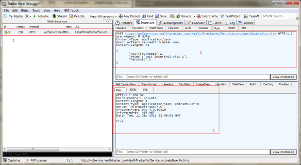
Fiddler Example – InsertActivity Operation Response
To view the Activity we just inserted, we need to call the ‘GetActivities’ operation, passing it the same ‘PersonId’ argument. In Fiddler, 1) select the ‘GET’ HTTP method, 2) input the URL for the ‘GetActivities’ operation including a value for the ‘PersonId’ argument, 3) select the desired version of HTTP (1.2), 4) input a Content-Type (JSON or XML) in the Request Headers section, and 5) select ‘Execute’. Same as before, the 6) Response should appear in the Web Sessions window. This time there is no Request body content.

Fiddler Example – GetActivities Operation Request
As before, executing the 1) Request should result in a 2) Response in the Web Sessions window. Doubling clicking on the Web Session should result in the display of the 3) Response in the lower left window. This method returns a JSON payload with each Activity, associated with the PersonId argument.

Fiddler Example – GetActivities Operation Response
You can use this same process to test all the other operations at the WCF Service’s endpoint. You can also save the Request message or complete Web Sessions in Fiddler should you need to re-test.
Conclusion
We now have a WCF Service deployed and running in IIS, and tested. The service’s operations can be called from any application capable of making an HTTP call. Thank you for taking the time to read this Post. I hope you found it beneficial.
Database First Development with Entity Framework 5 in Visual Studio 2012
Posted by Gary A. Stafford in .NET Development, Software Development on November 22, 2012
Build and test a Data Access Layer (DAL) using Entity Framework 5 and Database First Development in Visual Studio 2012. Use the Entity Framework Designer to build an ADO.NET Entity Data Model containing database tables, views, stored procedures, and scalar-valued functions. An updated version of this project’s source code, using EF6 is now available on GitHub. The GitHub repository contains all three Entity Framework blog posts.
![]()
Introduction
In the last post, we explored Microsoft’s new Entity Framework 5 with Code First Development. In this post, we will explore Entity Framework 5 with Database First Development. We will be using the same data model as before. However, this time instead of POCOs, we will start with a SQL Server 2008 R2 database and use the Entity Framework Designer to build an ADO.NET Entity Data Model (EDM). In addition to database tables, we will look at Entity Framework’s ability to support database views (virtual tables), stored procedures, and scalar-valued functions.
Download a complete copy of the post’s source code, with SQL scripts to create the database objects and populate the database with sample data, from DropBox.
Entity Framework’s Code First and Model First development offer many great options for .NET developers. However, in my experience, most enterprise-level application developers work with a Database First Development model. Using Database First Development, Entity Framework 5 (EF5) provides the ability to construct a powerful yet easy-to-implement data access layer (DAL) between the database and the business logic.
The steps involved in this example are as follows:
- Create the new SQL Server database;
- Create the database objects;
- Create a new C# Class Library Project in Visual Studio 2012 Solution;
- Add a new ADO.NET Entity Data Model to project;
- Create a new Database Connection;
- Import the database objects into the EDM;
- Modify the EDM to accommodate the scalar-valued functions;
- Populate the database with sample data;
- Validate the EDM using a Unit Test Project;
Below is a final view of the entire Solution for reference as you work through the post.

Solution Explorer View of Final Solution
The Database
Using SQL Server 2008 R2 Management Studio (SSMS), Toad for SQL, or similar application, create a new database, named ‘HealthTracker’. I left all the default database settings unchanged for this post.

Create the New Health Tracker Database
Next, execute the supplied sql script to populate the HealthTracker database with the necessary database objects. The script should insert the following objects: (6) tables, (1) view, (1) stored procedure, (3) scalar-valued functions, and all the necessary table relationships. All objects will be members of the default ‘dbo’ schema.

Database in SQL Server Object Viewer
Barring a few minor changes, this data model is identical to the one we built in the last post using Code First Development with POCOs. The below Database Diagram illustrates the one-to-many relationships between the tables. The tables are pluralized in the database, as opposed to singular in the ADO.NET Entity Data Model (Meals vs. Meal, People vs. Person, etc.). This is a common pattern with Entity Framework.

Database Diagram of Table Relationships
Optional: Setting Up Database Credentials
For security and simplicity, I choose to add a new Login, User, and Role to the database. This step is not necessary for this post. However, it is good to get into the habit of securing your database, using database Logins, Users, Roles, and Permissions. In addition, if you are planning to deploy the database and the DAL to other environments such as Test or Production, don’t tie your Solution to personal credentials, a machine-specific account, or to an administrative role in the database with overly broad permissions.
The Database User, DemoUser, is associated with the Login, DemoLogin. DemoUser is a member of the Database Role, DemoRole. I will use the DemoLogin account to connect the EDM to the database. DemoRole has the minimal required database permissions the Entity will need to function: Alter, Insert, Delete, Execute, Select, Update, and View definition. DemoUser only needs Connect permission. Again, this step is optional. You can use your own credentials if you choose.
Included with the downloadable code is a third sql script that should create the User, Role, Login, and required Permissions, if you choose to use them to follow along with the post.

Database Permissions for User and Role
The Data Access Layer
Following good software design principles, we will separate our concerns between Projects. We want to create a Data Access Layer (DAL), to act as an interface between our database and our business logic. We don’t want to interact with the data directly in our DAL Project. By separating the DAL into its own project, we can reference that project’s assembly (.dll) from any other project, be it another class library (our business logic), a WCF service, WPF, Silverlight or console application, or an ASP.NET site. To start, create a new Visual C# Class Library. Name it ‘HealthTracker.DataAccess.DbFirst’. Create a new Solution for the Project in the same dialog box, named ‘HealthTracker’.

New Visual C# Windows Class Library Project
First, install Entity Framework (System.Data.Entity namespace classes) into the Solution by right clicking on the Solution and selecting ‘Manage NuGet Packages for Solution…’. Install the ‘EntityFramework’ package. If you haven’t discovered the power of NuGet with Visual Studio, check out their site.

Manage NuGet Packages – Install EntityFramework Package
Next, add a new ‘ADO.NET Entity Data Model’ item, named ‘HealthTracker.edmx’, to the HealthTracker.DataAccess.DbFirst project. According to Microsoft, an .edmx file also contains information used by the ADO.NET Entity Data Model Designer (Entity Designer) to render a model graphically. An .edmx file is the combination of three metadata files: the conceptual schema definition language (CSDL), store schema definition language (SSDL), and mapping specification language (MSL) files. For more information, see .edmx File Overview (Entity Framework).

Adding the ADO.NET Entity Data Model to Project
Adding the ADO.NET Entity Data Model item will start the Entity Data Model Wizard. Since we are exploring Database First Development, select ‘Generate from Database’.

Entity Data Model Wizard – Generate from Database
Next, we will be prompted to choose a data connection. Since this is the first time we are accessing our newly created HealthTracker database, we need to create a new data connection. Select ‘New Connection…’

The options you chose in the ‘Connection Properties’ dialog window, such as the server and instance name, will depend on your own SQL Server configuration and the method you chose to log onto the server. As mentioned before, I will use the ‘DemoLogin’ account. The connection string will reside in the project’s app.config file. Make sure to always chose ‘Test Connection’ to verify you have configured the Data Connection properly.

New Connection – Database Connection Properties
Once the data connection is established, we are prompted to add the database objects to the EDM. Only add the objects that we created earlier with the sql script.

Entity Data Model Wizard – Choose Your Database Objects
When the import is complete, the EDM should look like the following in the Entity Designer. You should see the six table entities, with one-to-many associations between them, as well as the one view entity, ‘PersonSummaryView’. Each database object you imported is referred to as an entity. Drag the entities into any position you want on the Design surface.
HealthTracker Entity Data Model Diagram
Similarly, when the import is complete, the EDM should look like the following in the Model Browser.

Model Browser – View of the Entity Data Model
Stored Procedures
You recall we imported a stored procedure, ‘GetPersonSummary’. What happened to that object? In the Model Browser, double-click on the GetPersonSummary item under the Function Imports. The stored procedure was imported into the EDM by EF. The results the procedure returns from the database is associated with a new complex object type, ‘GetPersonSummary_Result’.

Function Import – Stored Procedure
Scalar Functions
If you view the sql code for the above stored procedure, ‘GetPersonSummary’, you will note it calls three scalar-valued functions. These three happen to be the three functions we imported into the EDM. Each function takes a single input parameter, ‘personId’, and returns an integer value – the count of Meals, Activities, and Hydrations for a that Person, based on their Id.
We can also call the scalar-valued functions directly. Unfortunately, in my experience, working scalar-valued functions in Entity Framework is still not as easy as tables, views, and stored procedures. I have found two methods to work with scalar-valued functions. The first method is a bit of hack in my opinion, but it works. The method is documented in several Internet posts, including this one on Stack Overflow.
This method requires some minor changes of the .edmx file’s xml, directly. To do so, right-click on the .edmx file and select ‘Open With…’, ‘XML (Text) Editor’. This is how the functions looks in the .edmx file before changes:
<Function Name="CountActivities" ReturnType="int" Aggregate="false" BuiltIn="false" NiladicFunction="false" IsComposable="false" ParameterTypeSemantics="AllowImplicitConversion" Schema="dbo">
    <Parameter Name="personId" Type="int" Mode="In" />
</Function>
<Function Name="CountHydrations" ReturnType="int" Aggregate="false" BuiltIn="false" NiladicFunction="false" IsComposable="true" ParameterTypeSemantics="AllowImplicitConversion" Schema="dbo">
    <Parameter Name="personId" Type="int" Mode="In" />
</Function>
<Function Name="CountMeals" ReturnType="int" Aggregate="false" BuiltIn="false" NiladicFunction="false" IsComposable="true" ParameterTypeSemantics="AllowImplicitConversion" Schema="dbo">
    <Parameter Name="personId" Type="int" Mode="In" />
</Function>
Remove the ‘ReturnType’ attribute from the <Function /> element. Then, add a <CommandText /> element to each of the <Function /> elements. See the modified .edmx file below for the contents of the <CommandText /> elements.
<Function Name="CountActivities" Aggregate="false" BuiltIn="false" NiladicFunction="false" IsComposable="false" ParameterTypeSemantics="AllowImplicitConversion" Schema="dbo">
    <CommandText>
        SELECT [dbo].[CountActivities] (@personId)
    </CommandText>
    <Parameter Name="personId" Type="int" Mode="In" />
</Function>
<Function Name="CountHydrations" Aggregate="false" BuiltIn="false" NiladicFunction="false" IsComposable="true" ParameterTypeSemantics="AllowImplicitConversion" Schema="dbo">
    <CommandText>
        SELECT [dbo].[CountHydrations] (@personId)
    </CommandText>
    <Parameter Name="personId" Type="int" Mode="In" />
</Function>
<Function Name="CountMeals" Aggregate="false" BuiltIn="false" NiladicFunction="false" IsComposable="true" ParameterTypeSemantics="AllowImplicitConversion" Schema="dbo">
    <CommandText>
        SELECT [dbo].[CountMeals] (@personId)
    </CommandText>
    <Parameter Name="personId" Type="int" Mode="In" />
</Function>
Next, in the Model Browser, right-click on the ‘Function Imports’ folder and select ‘Add Function Import…’ This brings up the ‘Add Function Import’ dialog window. We will import the ‘CountActivities’ scalar-valued function to show this method. Enter the following information in the dialog window and select Save:

Function Import – Scalar-valued Function
You can do the same for the other two scalar-valued functions, if you choose. We will only test the ‘CountActivities’ function, next with our Unit Tests. The downside of this method is the edits to the .edmx file will be lost when you update the EDM from the database. You will have to re-edit the .edmx file each time. This not a great solution.
The second method to call a scalar-valued function uses a feature of Entity Framework 5, the ‘Database.SqlQuery Method (String, Object[])’ Method. According to Microsoft, an instance of this class is obtained from an DbContext object and can be used to manage the actual database backing a DbContext or connection. Using ‘SqlQuery’ method, a raw SQL query that will return elements of the given generic type is created. The type can be any type that has properties that match the names of the columns returned from the query, or can be a simple primitive type.
Below is an example of the method’s use, similar to code in the Unit Test Project we will create next, to test our EDM.
using (HealthTrackerEntities context = new HealthTrackerEntities())
{
    string sqlQuery = "SELECT [dbo].[CountMeals] ({0})";
    Object[] parameters = { 1 };
    int activityCount = db.Database.SqlQuery<int>(sqlQuery, parameters).FirstOrDefault();
}
This method allows us to call the scalar-valued function directly from the database, just as we could any other object using a sql query. The downside of this method is that we are not really taking advantage of the EDM we constructed. It is easier than the first method and it doesn’t need continued changes if we update the EDM. Undoubtedly, there are better methods out there than I have presented here.
Testing the Entity Data Model
To confirm that the EDM is functioning properly, we will create and execute a series of Unit Tests. In reality, although we will be using Visual Studio’s Unit Test Project type, the tests are more like functional tests than true unit tests. This is especially true because we are writing the tests after we have completed development our DAL’s EDM.
We will perform minimal testing of the EDM’s tables, view, stored procedure, and scalar-valued functions, with a series of several simple tests. The tests are only meant to demonstrate the type of tests you could use across all entities in the Model to confirm various functions.
Sample Data
In SSMS or VS2012, execute the supplied sql script that populates the database with test data. The script contains a variety of Meal Types, Activity Types, People, Meals, Activities, and Hydrations table records. Note the script deletes all existing data from those tables. Below is a sample of the Meal table’s sample data.

Sample Meal Data
The Unit Test Project
After adding the sample data to the HealthTracker database, add a new Visual Studio 2012 Unit Test Project, named ‘HealthTracker.UnitTests’, to the ‘HealthTracker’ Solution.

Add New Unit Test Project to Solution
Next, add a Reference to the Unit Test Project from our DAL, the ‘HealthTracker.DataAccess.DbFirst’ Project. This step adds the ‘HealthTracker.DataAccess.DbFirst.dll’ assembly to our Unit Test Project.

Add Entity Data Model Project Reference to Unit Test Project
Next, we need to add the same Database Connection we used in the ‘HealthTracker.DataAccess.DbFirst’ Project, to this Project. I always forget this step and end up with a database connection error the first time I try to run a new project. Right-click on the Unit Test Project and select ‘Add New Item…’ Add an ‘Application Configuration File’ item, named ‘app.config’, to the Unit Test Project.

Add Application Configuration File to Unit Test Project
Open the corresponding Application Configuration File in the ‘HealthTracker.DataAccess.DbFirst’ Project and copy the <connectionStrings /> element to our Unit Test Project’s app.config file. The file’s contents should look similar to the following when complete (note, your ‘connectionString’ attribute will have different values).
<?xml version="1.0" encoding="utf-8" ?>
<configuration>
<connectionStrings>
<add name="HealthTrackerEntities" connectionString="metadata=res://*/HealthTracker.csdl|res://*/HealthTracker.ssdl|res://*/HealthTracker.msl;provider=System.Data.SqlClient;provider connection string="data source=gstafford-windows-laptop\DEVELOPMENT;initial catalog=HealthTracker;persist security info=True;user id=DemoLogin;password=DemoLogin123;MultipleActiveResultSets=True;App=EntityFramework"" providerName="System.Data.EntityClient" />
</connectionStrings>
</configuration>
Lastly, rename the default ‘UnitTest’ class in the Unit Test Project to ‘HealthTrackerUnitTests’. Enter or copy and paste the contents of the supplied HealthTrackerUnitTests.cs file to this file. The supplied file contains all the unit tests.
using System.Linq;
using Microsoft.VisualStudio.TestTools.UnitTesting;
using HealthTracker.DataAccess.DbFirst;

namespace HealthTracker.UnitTests
{
    [TestClass]
    public class HealthTrackerUnitTests
    {
        private const string PersonOriginal = "John Doe";
        private const string PersonNew = "New Person";
        private const string PersonNameUpdated = "Updated Name";

        /// <summary>
        /// Delete any non-sample People from the database created by previous tests
        /// </summary>
        [TestInitialize]
        public void RemoveNonSamplePeople()
        {
            using (var db = new HealthTrackerEntities())
            {
                var peopleToDelete = db.People
                    .Where(person => person.PersonId > 4);

                foreach (var personToDelete in peopleToDelete)
                {
                    db.People.Remove(personToDelete);
                }
                db.SaveChanges();
            }
        }

        /// <summary>
        /// Return the count of People in the database, which should be 4.
        /// </summary>
        [TestMethod]
        public void PersonCountTest()
        {
            using (var db = new HealthTrackerEntities())
            {
                var personCount = (db.People.Select(p => p)).Count();
                Assert.IsTrue(personCount > 0);
            }
        }

        /// <summary>
        /// Return the PersonId of 'John Doe', which should be is 1.
        /// </summary>
        [TestMethod]
        public void PersonIdTest()
        {
            using (var db = new HealthTrackerEntities())
            {
                var personId = db.People
                    .Where(person => person.Name == PersonOriginal)
                    .Select(person => person.PersonId)
                    .First();
                Assert.AreEqual(1, personId);
            }
        }
        /// <summary>
        /// Insert a new Person into the database.
        /// </summary>
        [TestMethod]
        public void PersonAddNewTest()
        {
            using (var db = new HealthTrackerEntities())
            {
                // Setup test
                db.People.Add(new Person { Name = PersonNew });
                db.SaveChanges();

                // Test 1
                var personCount = (db.People.Select(p => p)).Count();
                Assert.AreEqual(5, personCount);

                // Test 2
                var newPersonFound = db.People.FirstOrDefault(
                    person => person.Name == PersonNew);
                Assert.IsNotNull(newPersonFound);
            }
        }

        /// <summary>
        /// Update a Person's name in the database.
        /// </summary>
        [TestMethod]
        public void PersonUpdateNameTest()
        {
            using (var db = new HealthTrackerEntities())
            {
                // Setup test
                var personToUpdate = db.People.FirstOrDefault(
                    person => person.Name == PersonOriginal);

                if (personToUpdate != null) personToUpdate.Name = PersonNameUpdated;
                db.SaveChanges();

                // Test
                var updatedPerson = db.People.FirstOrDefault(
                    person => person.Name == PersonNameUpdated);
                Assert.IsNotNull(updatedPerson);

                // Tear down test
                var personToRevert = db.People.FirstOrDefault(
                    person => person.Name == PersonNameUpdated);

                if (personToRevert != null) personToRevert.Name = PersonOriginal;
                db.SaveChanges();
            }
        }

        /// <summary>
        /// Return the Meal count from PersonSummaryViews database view, which should be 21.
        /// </summary>
        [TestMethod]
        public void PersonSummaryViewTest()
        {
            using (var db = new HealthTrackerEntities())
            {
                var mealCount = (db.PersonSummaryViews
                    .Where(p => p.PersonId == 1)
                    .Select(p => p.MealsCount))
                    .First();
                Assert.AreEqual(21, mealCount);
            }
        }

        /// <summary>
        /// Call CountActivities scalar-valued function directly from in the database.
        /// </summary>
        [TestMethod]
        public void ActivtyCountFunctionFromDatabaseTest()
        {
            using (var db = new HealthTrackerEntities())
            {
                object[] parameters = { 1 };
                var activityCount = db.Database.SqlQuery<int>(
                    "SELECT [dbo].[CountActivities] ({0})",
                    parameters).FirstOrDefault();
                Assert.AreEqual(7, activityCount);
            }
        }

        /// <summary>
        /// Call CountActivities scalar-valued function from the Entity Data Model.
        /// </summary>
        [TestMethod]
        public void ActivtyCountFunctionFromEntityTest()
        {
            using (var db = new HealthTrackerEntities())
            {
                var activityCount = db.CountActivities(1).First();
                if (activityCount != null) activityCount = activityCount.Value;
                Assert.AreEqual(7, activityCount);
            }
        }
    }
}
When complete, build the Solution. Then finally, from the Test menu in the top Visual Studio menu bar, or by right clicking on the ‘HealthTrackerUnitTests’, run all Unit Tests. The test results should look like the following.

Test Explorer Showing Results of Unit Tests
Conclusion
Congratulations, we have built and tested a Data Access Layer using Entity Framework 5. The DAL can now be referenced from a middle-tier business assemble, WCF Service, or directly from a client application.
RESTful Mobile: Consuming Java EE RESTful Web Services Using jQuery Mobile
Posted by Gary A. Stafford in Java Development, Mobile HTML Development, Software Development on October 18, 2012
Use jQuery Mobile to build a mobile HTML website, capable of calling Jersey-specific Java EE RESTful web services and displaying JSONP in a mobile web browser.

Both NetBeans projects used in this post are available on DropBox. If you like DropBox, please use this link to sign up for a free 2 GB account. It will help me post more files to DropBox for future posts.
Background
In the previous two-part series, Returning JSONP from Java EE RESTful Web Services Using jQuery, Jersey, and GlassFish, we created a Jersey-specific RESTful web service from a database using EclipseLink (JPA 2.0 Reference Implementation), Jersey (JAX-RS Reference Implementation), JAXB, and Jackson Java JSON-processor. The service and associated entity class mapped to a copy of Microsoft SQL Server’s Adventure Works database. An HTML and jQuery-based client called the service, which returned a JSONP response payload. The JSON data it contained was formatted and displayed in a simple HTML table, in a web-browser.
Objectives
In this post, we will extend the previous example to the mobile platform. Using jQuery and jQuery Mobile JavaScript libraries, we will call two RESTful web services and display the resulting JSONP data using the common list/detail UX design pattern. We will display a list of Adventure Works employees. When the end-user clicks on an employee in the web-browser, a new page will display detailed demographic information about that employee.
Similar to the previous post, when the client website is accessed by the end-user in a mobile web browser, the client site’s HTML, CSS, and JavaScript files are downloaded and cached on the end-users machine. The JavaScript file, using jQuery and Ajax, makes a call to the RESTful web service, which returns JSON (or, JSONP in this case). This simulates a typical cross-domain situation where a client needs to consume RESTful web services from a remote source. This is not allowed by the same origin policy, but overcome by returning JSONP to the client, which wraps the JSON payload in a function call.
We will extend both the ‘JerseyRESTfulServices’ and ‘JerseyRESTfulClient’ projects we built in the last series of posts. Here are the high-level steps we will walk-through in this post:
- Create a second view (virtual table) in the Adventure Works database;
- Create a second entity class that maps to the new database view;
- Modify the existing entity class, adding JAXB and Jackson JSON annotations;
- Create a second Jersey-specific RESTful web service from the new entity using Jersey and Jackson;
- Modify the existing Jersey-specific RESTful web service, adding one new methods;
- Modify the web.xml file to allow us to use natural JSON notation;
- Implement a JAXBContext resolver to serialize the JSON using natural JSON notation;
- Create a simple list/detail two-page mobile HTML5 website using jQuery Mobile;
- Use jQuery, Ajax, and CSS to call, parse, and display the JSONP returned by the service.
RESTful Web Services Project
When we are done, the final RESTful web services projects will look like the screen-grab, below. It will contain (2) entity classes, (2) RESTful web service classes, (1) JAXBContext resolver class, and the web.xml configuration file:

JerseyRESTfulServices Project View in NetBeans
1: Create the Second Database View
Create a new database view, vEmployeeNames, in the Adventure Works database:
USE [AdventureWorks]
GO

SET ANSI_NULLS ON
GO

SET QUOTED_IDENTIFIER ON
GO

CREATE VIEW [HumanResources].[vEmployeeNames]
AS
SELECT TOP (100) PERCENT BusinessEntityID, REPLACE(RTRIM(LastName
     + COALESCE (' ' + Suffix + '', N'') + COALESCE (', ' + FirstName + ' ', N'')
     + COALESCE (MiddleName + ' ', N'')), '  ', ' ') AS FullName
FROM Person.Person
WHERE (PersonType = 'EM')
ORDER BY FullName
GO
2: Create the Second Entity
Add the new VEmployeeNames.java entity class, mapped to the vEmployeeNames database view, using NetBeans’ ‘Entity Classes from Database…’ wizard. Then, modify the class to match the code below.
package entities;

import java.io.Serializable;
import javax.persistence.Basic;
import javax.persistence.Column;
import javax.persistence.Entity;
import javax.persistence.Id;
import javax.persistence.NamedQueries;
import javax.persistence.NamedQuery;
import javax.persistence.Table;
import javax.validation.constraints.NotNull;
import javax.validation.constraints.Size;
import javax.xml.bind.annotation.XmlRootElement;
import javax.xml.bind.annotation.XmlType;

@Entity
@Table(name = "vEmployeeNames", catalog = "AdventureWorks", schema = "HumanResources")
@XmlRootElement(name = "vEmployeeNames")
@NamedQueries({
    @NamedQuery(name = "VEmployeeNames.findAll", query = "SELECT v FROM VEmployeeNames v"),
    @NamedQuery(name = "VEmployeeNames.findByBusinessEntityID", query = "SELECT v FROM VEmployeeNames v WHERE v.businessEntityID = :businessEntityID"),
    @NamedQuery(name = "VEmployeeNames.findByFullName", query = "SELECT v FROM VEmployeeNames v WHERE v.fullName = :fullName")})
public class VEmployeeNames implements Serializable {

    private static final long serialVersionUID = 1L;
    @Basic(optional = false)
    @NotNull
    @Id
    @Column(name = "BusinessEntityID")
    private int businessEntityID;
    @Basic(optional = false)
    @NotNull
    @Size(min = 1, max = 102)
    @Column(name = "FullName")
    private String fullName;

    public VEmployeeNames() {
    }

    public int getBusinessEntityID() {
        return businessEntityID;
    }

    public void setBusinessEntityID(int businessEntityID) {
        this.businessEntityID = businessEntityID;
    }

    public String getFullName() {
        return fullName;
    }

    public void setFullName(String fullName) {
        this.fullName = fullName;
    }
}
3: Modify the Existing Entity
Modify the existing VEmployee.java entity class to use JAXB and Jackson JSON Annotations as shown below (class code abridged). Note the addition of the @XmlType(propOrder = { "businessEntityID"... }) to the class, the @JsonProperty(value = ...) tags to each member variable, and the @Id tag to the businessEntityID, which serves as the entity’s primary key. We will see the advantages of the first two annotations later in the post when we return the JSON to the client.
package entities;

import java.io.Serializable;
import javax.persistence.Basic;
import javax.persistence.Entity;
import javax.persistence.Id;
import javax.persistence.NamedQueries;
import javax.persistence.NamedQuery;
import javax.persistence.Table;
import javax.validation.constraints.NotNull;
import javax.validation.constraints.Size;
import javax.xml.bind.annotation.XmlRootElement;
import javax.xml.bind.annotation.XmlType;
import org.codehaus.jackson.annotate.JsonProperty;

@Entity
@Table(name = "vEmployee", catalog = "AdventureWorks", schema = "HumanResources")
@XmlRootElement
@NamedQueries({
    @NamedQuery(name = "VEmployee.findAll", query = "SELECT v FROM VEmployee v"),
    ...})
    @XmlType(propOrder = {
    "businessEntityID",
    "title",
    "firstName",
    "middleName",
    "lastName",
    "suffix",
    "jobTitle",
    "phoneNumberType",
    "phoneNumber",
    "emailAddress",
    "emailPromotion",
    "addressLine1",
    "addressLine2",
    "city",
    "stateProvinceName",
    "postalCode",
    "countryRegionName",
    "additionalContactInfo"
})
public class VEmployee implements Serializable {

    private static final long serialVersionUID = 1L;
    @Basic(optional = false)
    @NotNull
    @Id
    @JsonProperty(value = "Employee ID")
    private int businessEntityID;
    @Size(max = 8)
    @JsonProperty(value = "Title")
    private String title;
    @Basic(optional = false)
    @NotNull
    @Size(min = 1, max = 50)
    @JsonProperty(value = "First Name")
    private String firstName;
    @Size(max = 50)
    @JsonProperty(value = "Middle Name")
    private String middleName;
    @Basic(optional = false)
    @NotNull
    @Size(min = 1, max = 50)
    @JsonProperty(value = "Last Name")
    private String lastName;
    @Size(max = 10)
    @JsonProperty(value = "Suffix")
    private String suffix;
    @Basic(optional = false)
    @NotNull
    @Size(min = 1, max = 50)
    @JsonProperty(value = "Job Title")
    private String jobTitle;
    @Size(max = 25)
    @JsonProperty(value = "Phone Number")
    private String phoneNumber;
    @Size(max = 50)
    @JsonProperty(value = "Phone Number Type")
    private String phoneNumberType;
    @Size(max = 50)
    @JsonProperty(value = "Email Address")
    private String emailAddress;
    @Basic(optional = false)
    @NotNull
    @JsonProperty(value = "Email Promotion")
    private int emailPromotion;
    @Basic(optional = false)
    @NotNull
    @Size(min = 1, max = 60)
    @JsonProperty(value = "Address Line 1")
    private String addressLine1;
    @Size(max = 60)
    @JsonProperty(value = "Address Line 2")
    private String addressLine2;
    @Basic(optional = false)
    @NotNull
    @Size(min = 1, max = 30)
    @JsonProperty(value = "City")
    private String city;
    @Basic(optional = false)
    @NotNull
    @Size(min = 1, max = 50)
    @JsonProperty(value = "State or Province Name")
    private String stateProvinceName;
    @Basic(optional = false)
    @NotNull
    @Size(min = 1, max = 15)
    @JsonProperty(value = "Postal Code")
    private String postalCode;
    @Basic(optional = false)
    @NotNull
    @Size(min = 1, max = 50)
    @JsonProperty(value = "Country or Region Name")
    private String countryRegionName;
    @Size(max = 2147483647)
    @JsonProperty(value = "Additional Contact Info")
    private String additionalContactInfo;

    public VEmployee() {
    }
    ...
}
4: Create the New RESTful Web Service
Add the new VEmployeeNamesFacadeREST.java RESTful web service class using NetBean’s ‘RESTful Web Services from Entity Classes…’ wizard. Then, modify the new class, adding the new findAllJSONP() method shown below (class code abridged). This method call the same super.findAll() method from the parent AbstractFacade.java class as the default findAll({id}) method. However, the findAllJSONP() method returns JSONP instead of XML or JSON, as findAll({id}) does. This is done by passing the results of super.findAll() to a new instance of Jersey’s JSONWithPadding() class (com.sun.jersey.api.json.JSONWithPadding).
package service;

import com.sun.jersey.api.json.JSONWithPadding;
import entities.VEmployeeNames;
import java.util.ArrayList;
import java.util.Collection;
import java.util.List;
import javax.ejb.Stateless;
import javax.persistence.EntityManager;
import javax.persistence.PersistenceContext;
import javax.persistence.criteria.CriteriaBuilder;
import javax.persistence.criteria.CriteriaQuery;
import javax.persistence.criteria.Root;
import javax.ws.rs.Consumes;
import javax.ws.rs.DELETE;
import javax.ws.rs.GET;
import javax.ws.rs.POST;
import javax.ws.rs.PUT;
import javax.ws.rs.Path;
import javax.ws.rs.PathParam;
import javax.ws.rs.Produces;
import javax.ws.rs.QueryParam;
import javax.ws.rs.core.GenericEntity;

@Stateless
@Path("entities.vemployeenames")
public class VEmployeeNamesFacadeREST extends AbstractFacade<VEmployeeNames> {
    ...
    @GET
    @Path("jsonp")
    @Produces({"application/javascript"})
    public JSONWithPadding findAllJSONP(@QueryParam("callback") String callback) {
        CriteriaBuilder cb = getEntityManager().getCriteriaBuilder();
        CriteriaQuery cq = cb.createQuery();
        Root empRoot = cq.from(VEmployeeNames.class);
        cq.select(empRoot);
        cq.orderBy(cb.asc(empRoot.get("fullName")));
        javax.persistence.Query q = getEntityManager().createQuery(cq);

        List<VEmployeeNames> employees = q.getResultList();
        return new JSONWithPadding(
                new GenericEntity<Collection<VEmployeeNames>>(employees) {
                }, callback);
    }
    ...
}
5: Modify the Existing Service
Modify the existing VEmployeeFacadeREST.java RESTful web service class, adding the findJSONP() method shown below (class code abridged). This method calls the same super.find({id}) in the AbstractFacade.java parent class as the default find({id}) method, but returns JSONP instead of XML or JSON. As with the previous service class above, this is done by passing the results to a new instance of Jersey’s JSONWithPadding() class (com.sun.jersey.api.json.JSONWithPadding). There are no changes required to the default AbstractFacade.java class.
package service;

import com.sun.jersey.api.json.JSONWithPadding;
import entities.VEmployee;
import java.util.ArrayList;
import java.util.Collection;
import java.util.List;
import javax.ejb.Stateless;
import javax.persistence.EntityManager;
import javax.persistence.PersistenceContext;
import javax.persistence.criteria.CriteriaBuilder;
import javax.persistence.criteria.CriteriaQuery;
import javax.persistence.criteria.Root;
import javax.ws.rs.Consumes;
import javax.ws.rs.DELETE;
import javax.ws.rs.GET;
import javax.ws.rs.POST;
import javax.ws.rs.PUT;
import javax.ws.rs.Path;
import javax.ws.rs.PathParam;
import javax.ws.rs.Produces;
import javax.ws.rs.QueryParam;
import javax.ws.rs.core.GenericEntity;

@Stateless
@Path("entities.vemployee")
public class VEmployeeFacadeREST extends AbstractFacade<VEmployee> {
    ...
    @GET
    @Path("{id}/jsonp")
    @Produces({"application/javascript"})
    public JSONWithPadding findJSONP(@PathParam("id") Integer id,
            @QueryParam("callback") String callback) {
        List<VEmployee> employees = new ArrayList<VEmployee>();
        employees.add(super.find(id));
        return new JSONWithPadding(
                new GenericEntity<Collection<VEmployee>>(employees) {
                }, callback);
    }
    ...
}
6: Allow POJO JSON Support
Add the JSONConfiguration.FEATURE_POJO_MAPPING servlet init parameter to web.xml, as shown below (xml abridged). According to the Jersey website, this will allow us to use POJO support, the easiest way to convert our Java Objects to JSON. It is based on the Jackson library.
<?xml version="1.0" encoding="UTF-8"?>
<web-app version="3.0" xmlns="http://java.sun.com/xml/ns/javaee" xmlns:xsi="http://www.w3.org/2001/XMLSchema-instance" xsi:schemaLocation="http://java.sun.com/xml/ns/javaee http://java.sun.com/xml/ns/javaee/web-app_3_0.xsd">
    <servlet>
        <servlet-name>ServletAdaptor</servlet-name>
        <servlet-class>com.sun.jersey.spi.container.servlet.ServletContainer</servlet-class>
        <init-param>
            <description>Multiple packages, separated by semicolon(;), can be specified in param-value</description>
            <param-name>com.sun.jersey.config.property.packages</param-name>
            <param-value>service</param-value>
        </init-param>
        <init-param>
            <param-name>com.sun.jersey.api.json.POJOMappingFeature</param-name>
            <param-value>true</param-value>
        </init-param>
        ...
7: Implement a JAXBContext Resolver
Create the VEmployeeFacadeREST.java JAXBContext resolver class, shown below. This allows us to serialize the JSON using natural JSON notation. A good explanation of the use of a JAXBContext resolver can be found on the Jersey website.
package config;

import com.sun.jersey.api.json.JSONConfiguration;
import com.sun.jersey.api.json.JSONJAXBContext;
import javax.ws.rs.ext.ContextResolver;
import javax.ws.rs.ext.Provider;
import javax.xml.bind.JAXBContext;

@Provider
public class JAXBContextResolver implements ContextResolver<JAXBContext> {

    JAXBContext jaxbContext;
    private Class[] types = {entities.VEmployee.class, entities.VEmployeeNames.class};

    public JAXBContextResolver() throws Exception {
        this.jaxbContext =
                new JSONJAXBContext(JSONConfiguration.natural().build(), types);
    }

    @Override
    public JAXBContext getContext(Class<?> objectType) {
        for (Class type : types) {
            if (type == objectType) {
                return jaxbContext;
            }
        }
        return null;
    }
}
What is Natural JSON Notation?
According to the Jersey website, “with natural notation, Jersey will automatically figure out how individual items need to be processed, so that you do not need to do any kind of manual configuration. Java arrays and lists are mapped into JSON arrays, even for single-element cases. Java numbers and booleans are correctly mapped into JSON numbers and booleans, and you do not need to bother with XML attributes, as in JSON, they keep the original names.”
What does that mean? Better yet, what does that look like? Here is an example of an employee record, first as plain old JAXB JSON in a JSONP wrapper:
callback({"vEmployee":{"businessEntityID":"211","firstName":"Hazem","middleName":"E","lastName":"Abolrous","jobTitle":"Quality Assurance Manager","phoneNumberType":"Work","phoneNumber":"869-555-0125","emailAddress":"hazem0@adventure-works.com","emailPromotion":"0","addressLine1":"5050 Mt. Wilson Way","city":"Kenmore","stateProvinceName":"Washington","postalCode":"98028","countryRegionName":"United States"}})
And second, JSON wrapped in JSONP, using Jersey’s natural notation. Note the differences in the way the parent vEmployee node, numbers, and nulls are handled in natural JSON notation.
callback([{"Employee ID":211,"Title":null,"First Name":"Hazem","Middle Name":"E","Last Name":"Abolrous","Suffix":null,"Job Title":"Quality Assurance Manager","Phone Number Type":"Work","Phone Number":"869-555-0125","Email Address":"hazem0@adventure-works.com","Email Promotion":0,"Address Line 1":"5050 Mt. Wilson Way","Address Line 2":null,"City":"Kenmore","State or Province Name":"Washington","Postal Code":"98028","Country or Region Name":"United States","Additional Contact Info":null}])
Mobile Client Project
When we are done with the mobile client, the final RESTful web services mobile client NetBeans projects should look like the screen-grab, below. Note the inclusion of jQuery Mobile 1.2.0. You will need to download the library and associated components, and install them in the project. I chose to keep them in a separate folder since there were several files included with the library. This example requires a few new features introduced in jQuery Mobile 1.2.0. Make sure to get this version or later.

JerseyRESTfulClient Project View in NetBeans
8: Create a List/Detail Mobile HTML Site
The process to display the data from the Adventure Works database in the mobile web browser is identical to the process used in the last series of posts. We are still using jQuery with Ajax, calling the same services, but with a few new methods. The biggest change is the use of jQuery Mobile to display the employee data. The jQuery Mobile library, especially with the release of 1.2.0, makes displaying data, quick and elegant. The library does all the hard work under the covers, with the features such as the listview control. We simply need to use jQuery and Ajax to retrieve the data and pass it to the control.
We will create three new files. They include the HTML, CSS, and JavaScript files. We add a ‘.m’ to the file names to differentiate them from the normal web browser files from the last post. As with the previous post, the HTML page and CSS file are minimal. The HTML page uses the jQuery Mobile multi-page template available on the jQuery Mobile website. Although it appears as two different web pages to the end-user, it is actually a single-page site.
Source code for employee.m.html:
<!DOCTYPE html>
<html>
    <head>
        <title>Employee List</title>
        <meta name="viewport" content="width=device-width, initial-scale=1">
        <meta http-equiv="Content-Type" content="text/html; charset=UTF-8">

        <link rel="stylesheet" href="jquery.mobile-1.2.0/jquery.mobile-1.2.0.min.css" />
        <link type="text/css" rel="stylesheet" href="employees.m.css" />

        <script src="jquery-1.8.2.min.js" type="text/javascript"></script>
        <script src="jquery.mobile-1.2.0/jquery.mobile-1.2.0.min.js" type="text/javascript"></script>
        <script src="employees.m.js" type="text/javascript"></script>
    </head>
    <body>
        <!-- Start of first page: #one -->
        <div data-role="page" id="one" data-theme="b">
            <div data-role="header" data-theme="b">
                <h1>Employee List</h1>
            </div><!-- /header -->
            <div data-role="content">
                <div id="errorMessage"></div>
                <div class="ui-grid-solo">
                    <form>
                        <ul data-role="listview" data-filter="true"
                            id="employeeList" data-theme="c" data-autodividers="true">
                        </ul>
                    </form>
                </div>
            </div><!-- /content -->
            <div data-role="footer" data-theme="b">
                <h4>Programmatic Ponderings, 2012</h4>
            </div><!-- /footer -->
        </div><!-- /page -->

        <!-- Start of second page: #two -->
        <div data-role="page" id="two" data-theme="c">
            <div data-role="header" data-theme="b">
                <a href="#one" data-icon="back">Return</a>
                <h1>Employee Detail</h1>
            </div><!-- /header -->
            <div data-role="content" data-theme="c">
                <div id="employeeDetail"></div>
            </div><!-- /content -->
            <div data-role="footer" data-theme="b">
                <h4>Programmatic Ponderings, 2012</h4>
            </div><!-- /footer -->
        </div><!-- /page two -->
    </body>
</html>
Source code for employee.m.css:
#employeeList {
    clear:both;
}

#employeeDetail div {
    padding-top: 2px;
    white-space: nowrap;
}

.field {
    margin-bottom: 0px;
    font-size: smaller;
    color: #707070;
}

.value {
    font-weight: bolder;
    padding-bottom: 12px;
    border-bottom: 1px #d0d0d0 solid;
}

.ui-block-a{
    padding-left: 6px;
    padding-right: 6px;
}

.ui-grid-a{
    padding-bottom: 12px;
    padding-top: -6px;
}
8: Retrieve, Parse, and Display the Data
The mobile JavaScript file below is identical in many ways to the JavaScript file used in the last series of posts for a non-mobile browser. One useful change we have made is the addition of two arguments to the function that calls jQuery.Ajax(). The address of the service (URI) that the jQuery.Ajax() method requests, and the function that Ajax calls after successful completion, are both passed into the callService(Uri, successFunction) function as arguments. This allows us to reuse the Ajax method for different purposes. In this case, we call the function once to populate the Employee List with the full names of the employees. We call it again to populate the Employee Detail page with demographic information of a single employee chosen from the Employee List. Both calls are to different URIs representing the two different RESTful web services, which in turn are associated with the two different entities, which in turn are mapped to the two different database views.
callService = function (uri, successFunction) {
        $.ajax({
            cache: true,
            url: uri,
            data: "{}",
            type: "GET",
            contentType: "application/javascript",
            dataType: "jsonp",
            error: ajaxCallFailed,
            failure: ajaxCallFailed,
            success: successFunction
        });
    };
The rest of the functions are self-explanatory. There are two calls to the jQuery Ajax method to return data from the service, two functions to parse and format the JSONP for display in the browser, and one jQuery method that adds click events to the Employee List. We perform a bit of string manipulation to imbed the employee id into the id property of each list item (li element. Later, when the end-user clicks on the employee name in the list, the employee id is extracted from the id property of the selected list item and passed back to the service to retrieve the employee detail. The HTML snippet below shows how a single employee row in the jQuery listview. Note the id property of the li element, id="empId_121", for employee id 121.
<li id="empId_121" class="ui-btn ui-btn-icon-right ui-li-has-arrow ui-li ui-btn-up-c"
    data-corners="false" data-shadow="false" data-iconshadow="true"
    data-wrapperels="div" data-icon="arrow-r" data-iconpos="right" data-theme="c">
    <div class="ui-btn-inner ui-li">
        <div class="ui-btn-text">
            <a class="ui-link-inherit" href="#">Ackerman, Pilar G</a>
        </div>
        <span class="ui-icon ui-icon-arrow-r ui-icon-shadow"> </span>
    </div>
</li>
To make this example work, you need to change the restfulWebServiceBaseUri variable to the server and port of the GlassFish domain running your RESTful web services. If you are testing the client locally on your mobile device, I suggest using the IP address for the GlassFish server versus a domain name, which your phone will be able to connect to in your local wireless environment. At least on the iPhone, there is no easy way to change the hosts file to provide local domain name resolution.
Source code for employee.m.js:
// ===========================================================================
//
// Author: Gary A. Stafford
// Website: http://www.programmaticponderings.com
// Description: Call RESTful Web Services from mobile HTML pages
// using jQuery mobile, Jersey, Jackson, and EclipseLink
//
// ===========================================================================
// Immediate function
(function () {
"use strict";
var restfulWebServiceBaseUri, employeeListFindAllUri, employeeByIdUri,
callService, ajaxCallFailed,
getEmployeeById, displayEmployeeList, displayEmployeeDetail;
// Base URI of RESTful web service
restfulWebServiceBaseUri = "http://your_server_name_or_ip:8080/JerseyRESTfulServices/webresources/";
// URI maps to service.VEmployeeNamesFacadeREST.findAllJSONP
employeeListFindAllUri = restfulWebServiceBaseUri + "entities.vemployeenames/jsonp";
// URI maps to service.VEmployeeFacadeREST.findJSONP
employeeByIdUri = restfulWebServiceBaseUri + "entities.vemployee/{id}/jsonp";
// Execute after the page one dom is fully loaded
$(".one").ready(function () {
// Retrieve employee list
callService(employeeListFindAllUri, displayEmployeeList);
// Attach onclick event to each row of employee list on page one
$("#employeeList").on("click", "li", function(event){
getEmployeeById($(this).attr("id").split("empId_").pop());
});
});
// Call a service URI and return JSONP to a function
callService = function (Uri, successFunction) {
$.ajax({
cache: true,
url: Uri,
data: "{}",
type: "GET",
contentType: "application/javascript",
dataType: "jsonp",
error: ajaxCallFailed,
failure: ajaxCallFailed,
success: successFunction
});
};
// Called if ajax call fails
ajaxCallFailed = function (jqXHR, textStatus) {
console.log("Error: " + textStatus);
console.log(jqXHR);
$("form").css("visibility", "hidden");
$("#errorMessage").empty().
append("Sorry, there was an error.").
css("color", "red");
};
// Display employee list on page one
displayEmployeeList = function (employee) {
var employeeList = "";
$.each(employee, function(index, employee) {
employeeList = employeeList.concat(
"<li id=empId_" + employee.businessEntityID.toString() + ">" +
"<a href='#'>" +
employee.fullName.toString() + "</a></li>");
});
$('#employeeList').empty();
$('#employeeList').append(employeeList).listview("refresh", true);
};
// Display employee detail on page two
displayEmployeeDetail = function(employee) {
$.mobile.loading( 'show', {
text: '',
textVisible: false,
theme: 'a',
html: ""
});
window.location = "#two";
var employeeDetail = "";
$.each(employee, function(key, value) {
$.each(value, function(key, value) {
if(!value) {
value = " ";
}
employeeDetail = employeeDetail.concat(
"<div class='detail'>" +
"<div class='field'>" + key + "</div>" +
"<div class='value'>" + value + "</div>" +
"</div>");
});
});
$("#employeeDetail").empty().append(employeeDetail);
};
// Retrieve employee detail based on employee id
getEmployeeById = function (employeeID) {
callService(employeeByIdUri.replace("{id}", employeeID), displayEmployeeDetail);
};
} ());
The Final Result
Viewed in Google’s Chrome for Mobile web browser on iOS 6, the previous project’s Employee List looks pretty bland and un-mobile like:

Previous Project as Viewed in Google Chrome for Mobile Web Browser
However, with a little jQuery Mobile magic you get a simple yet effective and highly functional mobile web presentation. Seen below on page one, the Employee List is displayed in Safari on an iPhone 4 with iOS 6. It features some of the new capabilities of jQuery Mobile 1.2.0’s improved listview, including autodividers.
Employee List
Here again is the Employee List using the jQuery Mobile 1.2.0’s improved listview search filter bar:

Employee List – Filtered
Here is the Employee Detail on page 2. Note the order and names of the fields. Remember previously when we annotated the VEmployeeNames.java entity with the @XmlType(propOrder = {"businessEntityID", ...}) to the class and the @JsonProperty(value = ...) tags to each member variable. This is the results of those efforts; our JSON is delivered pre-sorted and titled the way we want. No need to handle those functions on the client-side. This allows the client to be loosely-coupled to the data. The client simply displays whichever key/value pairs are delivered in the JSONP response payload.

Employee Detail

Employee Detail – Bottom
Returning JSONP from Java EE RESTful Web Services Using jQuery, Jersey, and GlassFish – Part 2 of 2
Posted by Gary A. Stafford in Java Development, Software Development on October 4, 2012
Create a Jersey-specific Java EE RESTful web service, and an HTML-based client to call the service and display JSONP. Test and deploy the service and the client to different remote instances of GlassFish.
Background
In part 1 of this series, we created a Jersey-specific RESTful web service from a database using NetBeans. The service returns JSONP in addition to JSON and XML. The service was deployed to a GlassFish domain, running on a Windows box. On this same box is the SQL Server instance, running the Adventure Works database, from which the service obtains data, via the entity class.
Objectives
In part two of this series, we will create a simple web client to consume and display the JSONP returned by the RESTful web service. There are many options available for creating a service consumer (client) depending on your development platform and project requirements. We will keep it simple, no complex, complied code, just HTML and JavaScript with jQuery, the well-known JavaScript library.
We will host the client on a separate GlassFish domain, running on an Ubuntu Linux VM using Oracle’s VM VirtualBox. This is a different machine than the service was installed on. When opened by the end-user in a web browser, the client files, including the JavaScript file that calls the service, are downloaded to the end-users machine. This will simulate a typical cross-domain situation where a client application needs to consume RESTful web services from a remote source. This is not allowed by the same origin policy, but overcome by returning JSONP to the client, which wraps the JSON payload in a function call.
Here are the high-level steps we will walk-through in part two:
- Create a simple HTML client using jQuery and ajax to call the RESTful web service;
- Add jQuery functionality to parse and display the JSONP returned by the service;
- Deploy the client to a separate remote instance of GlassFish using Apache Ant;
- Test the client’s ability to call the service across domains and display JSONP.
Creating the RESTful Web Service Client
New NetBeans Web Application Project
Create a new Java Web Application project in NetBeans. Name the project ‘JerseyRESTfulClient’. The choice of GlassFish server and domain where the project will be deployed is unimportant. We will use Apache Ant to deploy the client when we finish the building the project. By default, I chose my local instance of GlassFish, for testing purposes.

Create a New Web Application Project in NetBeans

Name and Location of New Web Application Project

Server and Settings of New Web Application Project

Optional Frameworks to Include in New Web Application Project

View of New Web Application Project in NetBeans
Adding Files to Project
The final client project will contains four new files:
- employees.html – HTML web page that displays a list of employees;
- employees.css – CSS information used to by employees.html;
- employees.js – JavaScript code used to by employees.html;
- jquery-1.8.2.min.js – jQuery 1.8.2 JavaScript library, minified.
First, we need to download and install jQuery. At the time of this post, jQuery 1.8.2 was the latest version. I installed the minified version (jquery-1.8.2.min.js) to save space.
Next, we will create the three new files (employees.html, employees.css, and employees.js), using the code below. When finished, we need to place all four files into the ‘Web Pages’ folder. The final project should look like:

Final Client Project View
HTML
The HTML file is the smallest of the three files. The HTML page references the CSS file, the JavaScript file, and the jQuery library file. The CSS file provides the presentation (look and feel) and JavaScript file, using jQuery, dynamically provides much of the content that the HTML page normally would contain.
<!DOCTYPE html>
<html>
    <head>
        <title>Employee List</title>
        <meta http-equiv="Content-Type" content="text/html; charset=UTF-8">
        <link type="text/css" rel="stylesheet" href="employees.css" />
        <script src="jquery-1.8.2.min.js" type="text/javascript"></script>
        <script src="employees.js" type="text/javascript"></script>
    </head>
    <body>
        <div id="pageTitle">Employee List</div>
        <div id="employeeList"></div>
    </body>
</html>
Cascading Style Sheets (CSS)
The CSS file is also pretty straight-forward. The pageTitle and employeeList id selectors and type selectors are used directly by the HTML page. The class selectors are all applied to the page by jQuery, in the JavaScript file.
body {
    font-family: sans-serif;
    font-size: small;
    padding-left: 6px;
}

span {
    padding: 6px;
    display: inline-block;
}

div {
    border-bottom: lightgray solid 1px;
}

#pageTitle {
    font-size: medium;
    font-weight: bold;
    padding: 12px 0px 12px 0px;
    border: none;
}

#employeeList {
    float: left;
    border: gray solid 1px;
}

.empId {
    width: 50px;
    text-align: center;
    border-right: lightgray solid 1px;
}

.name {
    width: 200px;
    border-right: lightgray solid 1px;
}

.jobTitle {
    width: 250px;
}

.header {
    font-weight: bold;
    border-bottom: gray solid 1px;
}

.even{
    background-color: rgba(0, 255, 128, 0.09);
}

.odd {
    background-color: rgba(0, 255, 128, 0.05);
}

.last {
    border-bottom: none;
}
jQuery and JavaScript
The JavaScript file is where all the magic happens. There are two primary functions. First, getEmployees, which calls the jQuery.ajax() method. According jQuery’s website, the jQuery Ajax method performs an asynchronous HTTP (Ajax) request. In this case, it calls our RESTful web service and returns JSONP. The jQuery Ajax method uses an HTTP GET method to request the following service resource (URI):
http://[your-service's-glassfish-server-name]:[your-service's-glassfish-domain-port]/JerseyRESTfulService/webresources/entities.vemployee/{from}/{to}/jsonp?callback={callback}.
The base (root) URI of the service in the URI above is as follows:
http://[server]:[port]/JerseyRESTfulService/webresources/entities.vemployee/
This is followed by a series of elements (nodes), {from}/{to}/jsonp, which together form a reference to a specific method in our service. As explained in the first post of this series, we include the /jsonp element to indicate we want to call the new findRangeJsonP method to return JSONP, as opposed to findRange method that returns JSON or XML. We pass the {from} path parameter a value of ‘0’ and the {to} path parameter a value of ‘10’.
Lastly, the method specifies the callback function name for the JSONP request, parseResponse, using the jsonpCallback setting. This value will be used instead of the random name automatically generated by jQuery. The callback function name is appended to the end of the URI as a query parameter. The final URL is as follows:
http://[server]:[port]/JerseyRESTfulService/webresources/entities.vemployee/0/10/jsonp?callback=parseResponse.
Note the use of the jsonpCallback setting is not required, or necessarily recommended by jQuery. Without it, jQuery generate a unique name as it will make it easier to manage the requests and provide callbacks and error handling. This example will work fine if you exclude the jsonpCallback: "parseResponse" setting.
getEmployees = function () {
    $.ajax({
        cache: true,
        url: restfulWebServiceURI,
        data: "{}",
        type: "GET",
        jsonpCallback: "parseResponse",
        contentType: "application/javascript",
        dataType: "jsonp",
        error: ajaxCallFailed,
        failure: ajaxCallFailed,
        success: parseResponse
    });
};
Once we have successfully returned the JSONP, the jQuery Ajax method calls the parseResponse(data) function, passing the JSON to the data argument. The parseResponse function iterates through the employee objects using the jQuery.each() method. Each field of data is surrounding with span and div tags, and concatenated to the employeeList string variable. The string is appended to the div tag with the id of ‘employeeList’, using jQuery’s .append() method. The result is an HTML table-like grid of employee names, ids, and job title, displayed on the employees.html page.
Lastly, we call the colorRows() function. This function uses jQuery’s .addClass(className) to assign CSS classes to objects in the DOM. The classes are added to stylize the grid with alternating row colors and other formatting.
parseResponse = function (data) {
    var employee = data.vEmployee;

    var employeeList = "";

    employeeList = employeeList.concat("<div class='header'>" +
        "<span class='empId'>Id</span>" +
        "<span class='name'>Employee Name</span>" +
        "<span class='jobTitle'>Job Title</span>" +
        "</div>");

    $.each(employee, function(index, employee) {
        employeeList = employeeList.concat("<div class='employee'>" +
            "<span class='empId'>" +
            employee.businessEntityID +
            "</span><span class='name'>" +
            employee.firstName + " " + employee.lastName +
            "</span><span class='jobTitle'>" +
            employee.jobTitle +
            "</span></div>");
    });

    $("#employeeList").empty();
    $("#employeeList").append(employeeList);
    colorRows();
};
Here are the complete JavaScript file contents:
// Immediate function
(function () {
    "use strict";

    var restfulWebServiceURI, getEmployees, ajaxCallFailed, colorRows, parseResponse;

    restfulWebServiceURI = "http://[your-service's-server-name]:[your-service's-port]/JerseyRESTfulService/webresources/entities.vemployee/0/10/jsonp";

    // Execute after the DOM is fully loaded
    $(document).ready(function () {
        getEmployees();
    });

    // Retrieve Employee List as JSONP
    getEmployees = function () {
        $.ajax({
            cache: true,
            url: restfulWebServiceURI,
            data: "{}",
            type: "GET",
            jsonpCallback: "parseResponse",
            contentType: "application/javascript",
            dataType: "jsonp",
            error: ajaxCallFailed,
            failure: ajaxCallFailed,
            success: parseResponse
        });
    };

    // Called if ajax call fails
    ajaxCallFailed = function (jqXHR, textStatus) {
        console.log("Error: " + textStatus);
        console.log(jqXHR);
        $("#employeeList").empty();
        $("#employeeList").append("Error: " + textStatus);
    };

    // Called if ajax call is successful
    parseResponse = function (data) {
        var employee = data.vEmployee;

        var employeeList = "";

        employeeList = employeeList.concat("<div class='header'>" +
            "<span class='empId'>Id</span>" +
            "<span class='name'>Employee Name</span>" +
            "<span class='jobTitle'>Job Title</span>" +
            "</div>");

        $.each(employee, function(index, employee) {
            employeeList = employeeList.concat("<div class='employee'>" +
                "<span class='empId'>" +
                employee.businessEntityID +
                "</span><span class='name'>" +
                employee.firstName + " " + employee.lastName +
                "</span><span class='jobTitle'>" +
                employee.jobTitle +
                "</span></div>");
        });

        $("#employeeList").empty();
        $("#employeeList").append(employeeList);
        colorRows();
    };

    // Styles the Employee List
    colorRows = function(){
        $("#employeeList .employee:odd").addClass("odd");
        $("#employeeList .employee:even").addClass("even");
        $("#employeeList .employee:last").addClass("last");
    };
} ());
Deployment to GlassFish
To deploy the RESTful web service client to GlassFish, run the following Apache Ant target. The target first calls the clean and dist targets to build the .war file, Then, the target calls GlassFish’s asadmin deploy command. It specifies the remote GlassFish server, admin port, admin user, admin password (in the password file), secure or insecure connection, the name of the container, and the name of the .war file to be deployed. Note that the server is different for the client than it was for the service in part 1 of the series.
<target name="glassfish-deploy-remote" depends="clean, dist"
        description="Build distribution (WAR) and deploy to GlassFish">
    <exec failonerror="true" executable="cmd" description="asadmin deploy">
        <arg value="/c" />
        <arg value="asadmin --host=[your-client's-glassfish-server-name]
            --port=[your-client's-glassfish-domain-admin-port]
            --user=admin --passwordfile=pwdfile --secure=false
            deploy --force=true --name=JerseyRESTfulClient
            --contextroot=/JerseyRESTfulClient dist\JerseyRESTfulClient.war" />
    </exec>
</target>
Although the client application does not require any Java code, JSP pages, or Servlets, I chose to use NetBeans’ Web Application project template to create the client and chose to create a .war file to make deployment to GlassFish easier. You could just install the four client files (jQuery, HTML, CSS, and JavaScript) on Apache, IIS, or any other web server as a simple HTML site.

Deploy Client Application to Remote GlassFish Domain Using Ant Target
Once the application is deployed to GlassFish, you should see the ‘JerseyRESTfulClient’ listed under the Applications tab within the remote server domain.

Client Application Deployed to Remote GlassFish Domain
We will call the client application from our browser. The client application, whose files are downloaded and are now local on our machine, will in turn will call the service. The URL to call the client is: http://[your-client's-glassfish-server-name]:[your-client's-glassfish-domain-port]/JerseyRESTfulClient/employees.html (see call-out 1, in the screen-grab, below).
Using Firefox with Firebug, we can observe a few important items once the results are displayed (see the screen-grab, below):
- The four client files (jQuery, HTML, CSS, and JavaScript) are cached after the first time the client URL loads, but the jQuery Ajax service call is never cached (call-out 2);
- All the client application files are loaded from one domain, while the service is called from another domain (call-out 3);
- The ‘parseRequest’ callback function in the JSONP response payload, wraps the JSON data (call-out 4).
")
Employee List Displayed by Client Application in Firefox
The JSONP returned by the service to the client (abridged for length):
parseResponse({"vEmployee":[{"addressLine1":"4350 Minute Dr.","businessEntityID":"1","city":"Newport Hills","countryRegionName":"United States","emailAddress":"ken0@adventure-works.com","emailPromotion":"0","firstName":"Ken","jobTitle":"Chief Executive Officer","lastName":"Sánchez","middleName":"J","phoneNumber":"697-555-0142","phoneNumberType":"Cell","postalCode":"98006","stateProvinceName":"Washington"},{"addressLine1":"7559 Worth Ct.","businessEntityID":"2","city":"Renton","countryRegionName":"United States","emailAddress":"terri0@adventure-works.com","emailPromotion":"1","firstName":"Terri","jobTitle":"Vice President of Engineering","lastName":"Duffy","middleName":"Lee","phoneNumber":"819-555-0175","phoneNumberType":"Work","postalCode":"98055","stateProvinceName":"Washington"},{...}]})
The JSON passed to the parseResponse(data) function’s data argument (abridged for length):
{"vEmployee":[{"addressLine1":"4350 Minute Dr.","businessEntityID":"1","city":"Newport Hills","countryRegionName":"United States","emailAddress":"ken0@adventure-works.com","emailPromotion":"0","firstName":"Ken","jobTitle":"Chief Executive Officer","lastName":"Sánchez","middleName":"J","phoneNumber":"697-555-0142","phoneNumberType":"Cell","postalCode":"98006","stateProvinceName":"Washington"},{"addressLine1":"7559 Worth Ct.","businessEntityID":"2","city":"Renton","countryRegionName":"United States","emailAddress":"terri0@adventure-works.com","emailPromotion":"1","firstName":"Terri","jobTitle":"Vice President of Engineering","lastName":"Duffy","middleName":"Lee","phoneNumber":"819-555-0175","phoneNumberType":"Work","postalCode":"98055","stateProvinceName":"Washington"},{...}]}
Firebug also allows us to view the JSON in a more structured and object-oriented view:
")
Firefox Showing formatted JSON Data Using Firebug
Conclusion
We have successfully built and deployed a RESTful web service to one GlassFish domain, capable of returning JSONP. We have also built and deployed an HTML client to another GlassFish domain, capable of calling the service and displaying the JSONP. The service and client in this example have very minimal functionality. However, the service can easily be scaled to include multiple entities and RESTful services. The client’s capability can be expanded to perform a full array of CRUD operations on the database, through the RESTful web service(s).
Returning JSONP from Java EE RESTful Web Services Using jQuery, Jersey, and GlassFish – Part 1 of 2
Posted by Gary A. Stafford in Java Development, Software Development on October 1, 2012
Create a Jersey-specific Java EE RESTful web service and an HTML-based client to call the service and display JSONP. Test and deploy the service and the client to different remote instances of GlassFish.
Background
According to Wikipedia, JSONP (JSON with Padding) is a complement to the base JSON (JavaScript Object Notation) data format. It provides a method to request data from a server in a different domain, something prohibited by typical web browsers because of the same origin policy.
Jersey is the open source, production quality, JAX-RS (JSR 311) Reference Implementation for building RESTful Web services on the Java platform according to jersey.java.net. Jersey is a core component of GlassFish.
What do these two things have in common? One of the key features of Jersey is its ability to return JSONP. According to Oracle’s documentation, using Jersey, if an instance is returned by a resource method and the most acceptable media type is one of application/javascript, application/x-javascript, text/ecmascript, application/ecmascript or text/jscript then the object that is contained by the instance is serialized as JSON (if supported, using the application/json media type) and the result is wrapped around a JavaScript callback function, whose name by default is “callback”. Otherwise, the object is serialized directly according to the most acceptable media type. This means that an instance can be used to produce the media types application/json, application/xml in addition to application.
There is plenty of opinions on the Internet about the pros and cons of using JSONP over other alternatives to get around the same origin policy. Regardless of the cons, JSONP, with the help of Jersey, provides the ability to call a RESTful web service from a remote server, without a lot of additional coding or security considerations.
Objectives
Similar to GlassFish, Jersey is also tightly integrated into NetBeans. NetBeans provides the option to use Jersey-specific features when creating RESTful web services. According to documentation, NetBeans will generate a web.xml deployment descriptor and to register the RESTful services in that deployment descriptor instead of generating an application configuration class. In this post, we will create Jersey-specific RESTful web service from a database using NetBeans. The service will return JSONP in addition to JSON and XML.
In addition to creating the RESTful web service, in part 2 of this series, we will create a simple web client to display the JSONP returned by the service. There are many options available for creating clients, depending on your development platform and project requirements. We will keep it simple – no complex compiled code, just simple JavaScript using Ajax and jQuery, the well-known JavaScript library.
We will host the RESTful web service on one GlassFish domain, running on a Windows box, along with the SQL Server database. We will host the client on a second GlassFish domain, running on an Ubuntu Linux VM using Oracle’s VM VirtualBox. This is a different machine than the service was installed on. When opened by the end-user in a web browser, the client files, including the JavaScript file that calls the service, are downloaded to the end-users machine. This will simulate a typical cross-domain situation where a client application needs to consume RESTful web services from a remote source. This is not allowed by the same origin policy, but overcome by returning JSONP to the client, which wraps the JSON payload in a function call.
Demonstration
Here are the high-level steps we will walk-through in this two-part series of posts:
- In a new RESTful web service web application project,
- Create an entity class from the Adventure Works database using EclipseLink;
- Create a Jersey-specific RESTful web service using the entity class using Jersey and JAXB;
- Add a new method to service, which leverages Jersey and Jackson’s abilities to return JSONP;
- Deploy the RESTful web service to a remote instance of GlassFish, using Apache Ant;
- Test the RESTful web service using cURL.
- In a new RESTful web service client web application project,
- Create a simple HTML client using jQuery and Ajax to call the RESTful web service;
- Add jQuery functionality to parse and display the JSONP returned by the service;
- Deploy the client to a separate remote instance of GlassFish using Apache Ant;
- Test the client’s ability to call the service across domains and display JSONP.
To demonstrate the example in this post, I have the follow applications installed, configured, and running in my development environment:
- Microsoft SQL Server 2008 R2 (www.microsoft.com/sqlserver)
- Microsoft’s Adventure Works 2008 R2 Sample Database (msftdbprodsamples.codeplex.com)
- Microsoft JDBC Driver 4.0 for SQL Server (msdn.microsoft.com/en-us/sqlserver/aa937724.aspx)
- NetBeans 7.2 Open Source IDE (netbeans.org)
- Apache Any 1.82 (installed with NetBeans or downloaded separately from ant.apache.org)
- GlassFish 3.2.2.2 Open Source Edition Application Server (installed with NetBeans or downloaded separately from glassfish.java.net)
For the database we will use the Microsoft SQL Server 2008 R2 Adventure Works database I’ve used in the past few posts. For more on the Adventure Works database, see my post, ‘Convert VS 2010 Database Project to SSDT and Automate Publishing with Jenkins – Part 1/3’. Not using SQL Server? Once you’ve created your data source, most remaining steps in this post are independent of the database you choose, be it MySQL, Oracle, Microsoft SQL Server, Derby, etc.
For a full explanation of the use of Jersey and Jackson JSON Processor, for non-Maven developers, as this post demonstrates, see this link to the Jersey 1.8 User Guide. It discusses several relevant topics to this article: Java Architecture for XML Binding (JAXB), JSON serialization, and natural JSON notation (or, convention). See this link from the User Guide, for more on natural JSON notation. Note this example does not implement natural JSON notation functionality.
Creating the RESTful Web Service
New NetBeans Web Application Project
Create a new Java Web Application project in NetBeans. Name the project. I named mine ‘JerseyRESTfulService’. The choice of GlassFish server and domain where the project will be deployed is unimportant. We will use Apache Ant to deploy the service when we finish the building the project. By default, I chose my local instance of GlassFish, for testing purposes.

Create a New Web Application Project in NetBeans

Name and Location of New Web Application Project

Server and Settings of New Web Application Project

Optional Frameworks to Include in New Web Application Project

View of New Web Application Project in NetBeans
Create Entity Class from Database
Right-click on the project again and select ‘New’ -> ‘Other…’. From the list of Categories, select ‘Persistence’. From the list of Persistence choices, choose ‘Entity Classes from Database’. Click Next.

Create Entity Classes from the Database
Before we can choose which database table we want from the Adventure Works database to create entity class, we must create a connection to the database – a SQL Server Data Source. Click on the Data Source drop down and select ‘New Data Source…’. Give a Java Naming and Directory Interface (JNDI) name for the data source. I called mine ‘AdventureWorks_HumanResources’. Click on the ‘Database Connection’ drop down menu, select ‘New Database Connection…’.

Select Database Tables for Entity Classes (No Data Source Exists Yet)

Create and Name a New Data Source
This starts the ‘New Connection Wizard’. The first screen, ‘Locate Driver’, is where we point NetBeans to the Microsoft JDBC Driver 4.0 for SQL Server Driver. Locate the sqljdbc4.jar file.

Add the Microsoft JDBC Driver 4.0 for SQL Server Jar File
On the next screen, ‘Customize the Connection’, input the required SQL Server information. The host is the machine your instance of SQL Server is installed on, such as ‘localhost’. The instance is the name of the SQL Server instance in which the Adventure Works database is installed, such as ‘Development’. Once you complete the form, click ‘Test Connection’. If it doesn’t succeed, check your settings, again. Keep in mind, ‘localhost’ will only work if your SQL Server instance is local to your GlassFish server instance where the service will be deployed. If it is on a separate server, make sure to use that server’s IP address or domain name.

Configure New Database Connection
As I mentioned in an earlier post, the SQL Server Data Source forces you to select a single database schema. On the ‘Choose Database Schema’ screen, select the ‘HumanResources’ schema. The database tables you will be able to reference from you entity classes are limited to just this schema, when using this data source. To reference other schemas, you will need to create more data sources.

Select Human Resources Database Schema
Back in the ‘New Entity Classes from Database’ window, you will now have the ‘AdventureWorks’ data source selected as the Data Source. After a few seconds of processing, all ‘Available Tables’ within the ‘HumanResources’ schema are displayed. Choose the ‘vEmployee(view)’. A database view is a virtual database table. Note the Entity ID message. We will need to do an extra step later on, to use the entity class built from the database view.

Choice of Database Tables and Views from Human Resources Schema

Choose the ‘vEmployee(view)’ Database View
On the next screen, ‘Entity Classes’, in the ‘New Entity Classes from Database’ window, select or create the Package to place the individual entity classes into. I chose to call mine ‘entities’.

Select/Create the Package Location for the Entity Class
On the next screen, ‘Mapping Options’, choose ‘Fully Qualified Database Table Names’. Without this option selected, I have had problems trying to make the RESTful web services function properly. This is also the reason I chose to create the entity classes first, and then create the RESTful web services, separately. NetBeans has an option that combines these two tasks into a single step, by choosing ‘RESTful Web Services from Database’. However, the ‘Fully Qualified Database Table Names’ option is not available on the equivalent screen, using that process (at least in my version of NetBeans 7.2). I prefer the two-step approach.

Select the ‘Fully Qualified Database Table Names’ Mapping Options
Click finished. You have successfully created the SQL Server data source and entity classes.

Project View of New VEmployee Entity Class
If you recall, I mentioned a problem with the entity class we created from the database view. To avoid an error when you build and deploy your project to GlassFish, we need to make a small change to the VEmployee.java entity class. Entity classes need a unique identifier, a primary key (or, Entity ID) identified. Since this entity class was built from database view, as opposed to database table, it lacks a primary key. To fix, annotate the businessEntityID field with @Id. This indicates that businessEntityID is the primary key (Entity ID) for this class. The field, businessEntityID, must contain unique values, for this to work properly. NetBeans will make the suggested correction for you, if you allow it.

Fix the Entity Class’s Missing Primary Key (Entity ID)

Fix the Entity Class’s Missing Primary Key (Entity ID)

Entity Class With Primary Key (Entity ID)
The JPA Persistence Unit is found in the ‘persistence.xml’ file in the ‘Configuration Files’ folder. This file describes the Persistence Unit (PU). The PU serves to register the project’s persistable entity class, which are referred to by JPA as ‘managed classes’.

View of New JPA Persistence Unit
The data source we created, which will be deployed to GlassFish, is referred to as a JDBC Resource and JDBC Connection Pool. This information is stored in the ‘glassfish-resources.xml’.

View of New JDBC Resource and JDBC Connection Pool
Create RESTful Web Service
Now that have a SQL Server Data Source and our entity class, we will create the RESTful web service. Right-click on the project and select ‘New’ -> ‘Other…’ -> ‘Persistence’ -> ‘RESTful Web Services from ‘Entity Classes’. You will see the entity class we just created, from which to choose. Add the entity class.

Create RESTful Web Services from Entity Classes

Choose from List of Available Entity Classes

Choose the VEmployee Entity Class
On the next screen, select or create the Resource Package to store the service class in; I called mine ‘service’. Select the ‘Use Jersey Specific Features’ option.

Select/Create the Service’s Package Location and Select the Option to ‘Use Jersey Specific Features’
That’s it. You now have a Jersey-specific RESTful web service and the corresponding Enterprise Bean and Façade service class in the project.

Project View of New RESTful Web Service and Associated Files
NetBeans provides an easy way to test the RESTful web services, locally. Right-click on the ‘RESTful Web Services’ project folder within the main project, and select ‘Test RESTful Web Services’. Select the first option, ‘Locally Generated Test Client’, in the ‘Configure REST Test Client’ pop-up window. NetBeans will use the locally configured GlassFish instance to deploy and test the service.
NetBeans opens a web browser window and display the RESTful URIs (Universal Resource Identifier) for the service in a tree structure. There is a parent URI, ‘entities.vemployee’. Selecting this URI will return all employees from the vEmployee database view. The ‘entities.vemployee’ URI has additional children URIs grouped under it, including ‘{id}’, ‘count’, and ‘{from/to}’, each mapped to separate methods in the service class.
Click on the ‘{id}’ URI. Choose the HTTP ‘GET()’ request method from the drop-down, enter ‘1’ for ‘id’, and click the ‘Test’ button. The service should return a status of ‘200 (OK)’, along with xml output containing information on all the Adventure Works employees. Change the MIME type to ‘application/json’. This should return the same result, formatted as JSON. Congratulation, the RESTful web services have just returned data to your browser from the SQL Server Adventure Works database, using the entity classes and data source you created.
Are they URIs or URLs? I found this excellent post that does a very good job explaining the difference between the URL (how to get there) and the URI (the resource), which is part of the URL.

Test the RESTful Web Service Locally in NetBeans (XML Response Shown)

Test the RESTful Web Service Locally in NetBeans (JSON Response Shown)
Using Jersey for JSONP
GlassFish comes with the jersey-core.jar installed. In order to deliver JSONP, we also need to import and use com.sun.jersey.api.json.JSONWithPadding package from jersey-json.jar. I downloaded and installed version 1.8. You can download the jar from several locations. I chose to download it from www.java2.com. You can also download from the download.java.net Maven2 repository.

Add the Jersey JSON Jar File to the Project
The com.sun.jersey.api.json.JSONWithPadding package has dependencies two Jackson JSON Processor jars. You will also need to download the necessary Jackson JSON Processor jars. They are the jackson-core-asl-1.9.8.jar and jackson-mapper-asl-1.9.8.jar. At the time of this post, I downloaded the latest 1.9.8 versions from the grepcode.com Maven2 repository.

Add the two Jackson JSON Processor Jar Files to the Project
Create New JSONP Method
NetBeans creates several default methods in the VEmployeeFacadeREST class. One of those is the findRange method. The method accepts two integer parameters, from and to. The parameter values are extracted from the URL (JAX-RS @Path annotation). The parameters are called path parameters (@PathParam). The method returns a List of VEmployee objects (List<VEmployee>). The findRange method can return two MIME types, XML and JSON (@Produces). The List<VEmployee> is serialized in either format and returned to the caller.
@GET
@Path("{from}/{to}")
@Produces({"application/xml", "application/json"})
public List<VEmployee> findRange(@PathParam("from") Integer from, @PathParam("to") Integer to) {
    return super.findRange(new int[]{from, to});
}
Neither XML nor JSON will do, we want to return JSONP. Well, using the JSONWithPadding class we can do just that. We will copy and re-write the findRange method to return JSONP. The new findRangeJsonP method looks similar to the findRange. However instead of returning a List<VEmployee>, the new method returns an instance of the JSONWithPadding class. Since List<E> extends Collection<E>, we make the same call as the first method, then cast the List<VEmployee> to Collection<VEmployee>. We then wrap the Collection in a GenericEntity<T>, which extends Object. The GenericEntity<T> represents a response entity of a generic type T. This is used to instantiate a new instance of the JSONWithPadding class, using the JSONWithPadding(Object jsonSource, String callbackName) constructor. The JSONWithPadding instance, which contains serialized JSON wrapped with the callback function, is returned to the client.
@GET
@Path("{from}/{to}/jsonp")
@Produces({"application/javascript"})
public JSONWithPadding findRangeJsonP(@PathParam("from") Integer from,
        @PathParam("to") Integer to, @QueryParam("callback") String callback) {
    Collection<VEmployee> employees = super.findRange(new int[]{from, to});
    return new JSONWithPadding(new GenericEntity<Collection<VEmployee>>(employees) {
    }, callback);
}
We have added a two new parts to the ‘from/to’ URL. First, we added ‘/jsonp’ to the end to signify the new findRangeJsonP method is to be called, instead of the original findRange method. Secondly, we added a new ‘callback’ query parameter (@QueryParam). The ‘callback’ parameter will pass in the name of the callback function, which will then be returned with the JSONP payload. The new URL format is as follows:
http://[your-service's-glassfish-server-name]:[your-service's-glassfish-domain-port]/JerseyRESTfulService/webresources/entities.vemployee/{from}/{to}/jsonp?callback={callback}

Add the Following Jersey JSONP Method to the RESTful Web Service Class

Adding the Method Requires Importing the ‘JSONWithPadding’ Library
Deployment to GlassFish
To deploy the RESTful web service to GlassFish, run the following Apache Ant target. The target first calls the clean and dist targets to build the .war file, Then, the target calls GlassFish’s asadmin deploy command. It specifies the remote GlassFish server, admin port, admin user, admin password (in the password file), secure or insecure connection, the name of the container, and the name of the .war file to be deployed. Note that the server is different for the service than it will be for the client in part 2 of the series.
<target name="glassfish-deploy-remote" depends="clean, dist"
        description="Build distribution (WAR) and deploy to GlassFish">
    <exec failonerror="true" executable="cmd" description="asadmin deploy">
        <arg value="/c" />
        <arg value="asadmin --host=[your-service's-glassfish-server-name]
            --port=[your-service's-glassfish-domain-admin-port]
            --user=admin --passwordfile=pwdfile --secure=false
            deploy --force=true --name=JerseyRESTfulService
            --contextroot=/JerseyRESTfulServicedist\JerseyRESTfulService.war" />
    </exec>
</target>

Deploy RESTful Web Service to Remote GlassFish Server Using Apache Ant Target
In GlassFish, you should see the several new elements: 1) JerseyRESTfulService Application, 2) AdventureWorks_HumanResources JDBC Resource, 3) microsoft_sql_AdventureWorks_aw_devPool JDBC Connection Pool. These are the elements that were deployed by Ant. Also note, 4) the RESTful web service class, VEmployeeFacadeREST, is an EJB StatelessSessionBean.

RESTful Web Service Deployed to Remote GlassFish Server
Test the Service with cURL
What is the easiest way to test our RESTful web service without a client? Answer, cURL, the free open-source URL tool. According to the website, “curl is a command line tool for transferring data with URL syntax, supporting DICT, FILE, FTP, FTPS, Gopher, HTTP, HTTPS, IMAP, IMAPS, LDAP, LDAPS, POP3, POP3S, RTMP, RTSP, SCP, SFTP, SMTP, SMTPS, Telnet and TFTP. curl supports SSL certificates, HTTP POST, HTTP PUT, FTP uploading, HTTP form based upload, proxies, cookies, user+password authentication (Basic, Digest, NTLM, Negotiate, kerberos…), file transfer resume, proxy tunneling and a busload of other useful tricks.”
To use cURL, download and unzip the cURL package to your system’s Programs directory. Add the cURL directory path to your system’s PATH environmental variable. Better yet, create a CURL_HOME environmental variable and add that reference to the PATH variable, as I did. Adding the the cURL directory path to PATH allows you to call the cURL.exe application, directly from the command line.

Add the cURL Directory Path to the ‘PATH’ Environmental Variable
With cURL installed, we can call the RESTful web service from the command line. To test the service’s new method, call it with the following cURL command:
curl -i -H "Accept: application/x-javascript" -X GET http://[your-service's-glassfish-server-name]:[your-service's-glassfish-domain-port]/JerseyRESTfulService/webresources/entities.vemployee/1/3/jsonp?callback=parseResponse

Using cURL to Call RESTful Web Service and Return JSONP
Using cURL is great for testing the RESTful web service. However, the command line results are hard to read. I recommend copy the cURL results into NotePad++ with the JSON Viewer Plugin. Like the NotePad++ XML plugin, the JSON plugin will format the JSONP and provide a tree view of the data structure.

Notepad++ Displaying JSONP Using the JSON Viewer Plugin
Conclusion
Congratulations! You have created and deployed a RESTful web service with a method capable of returning JSONP. In part 2 of this series, we will create a client to call the RESTful web service and display the JSONP response payload. There are many options available for creating clients, depending on your development platform and project requirements. We will keep it simple – no complex, compiled code, just simple JavaScript using Ajax and jQuery, the well-known JavaScript library.
Connecting Java EE RESTful Web Services to Microsoft SQL Server Using NetBeans and GlassFish
Posted by Gary A. Stafford in Java Development, Software Development on September 15, 2012
Connecting Java EE RESTful web services, hosted on GlassFish, to Microsoft SQL Server – a high level overview. Demonstrate the creation of a Web Application project in NetBeans, including a SQL Server data source, entity classes from a SQL database, and RESTful web services. Show how to test and deploy the project to GlassFish.
Introduction
In a previous post, Connecting Java EE to SQL Server with Microsoft’s JDBC Driver 4.0, I demonstrated how Microsoft’s JDBC Driver 4.0 can connect Java-based RESTful web services to Microsoft SQL Server. In a more recent post, Calling Microsoft SQL Server Stored Procedures from a Java Application Using JDBC, I demonstrated the use of JDBC to call stored procedures from a Java application. In this post, I am going to offer a high-level, end-to-end overview on how to create and connect Java EE RESTful web services, hosted on GlassFish, to SQL Server. The goals of post are:
- Demonstrate the use of Microsoft’s JDBC Driver 4.0 to connect a Java-based application to SQL Server 2008 R2;
- Demonstrate the use of NetBeans to:
- Create a SQL Server Data Source;
- Create entity classes from the SQL Server database using the SQL Server Data Source;
- Create RESTful web services using JAX-RS, which communicate with database, through the entity classes;
- Compile and deploy the data source, entities, and services to GlassFish;
- Test the RESTful Web Services locally in NetBeans, and once deployed, in GlassFish.
Setting up the Post’s Example
To demonstrate the example in this post, I have the follow applications installed, configured, and running in my development environment:
- Microsoft SQL Server 2008 R2 (www.microsoft.com/sqlserver)
- Microsoft’s Adventure Works 2008 R2 Sample Database (msftdbprodsamples.codeplex.com)
- Microsoft JDBC Driver 4.0 for SQL Server (msdn.microsoft.com/en-us/sqlserver/aa937724.aspx)
- NetBeans 7.2 Open Source IDE (netbeans.org)
- Apache Any 1.82 (installed with NetBeans or downloaded separately from ant.apache.org)
- GlassFish 3.2.2.2 Open Source Edition Application Server (installed with NetBeans or downloaded separately from glassfish.java.net)
If you have any questions about installing and configuring the Adventure Works database, please refer to my post, Convert VS 2010 Database Project to SSDT and Automate Publishing with Jenkins – Part 1/3. The post takes you through creating a SQL Server 2008 R2 instance (entitled ‘Development’), installing the Adventure Works database, and creating a database user (‘aw-dev’). Also, refer to my earlier post, Connecting Java EE to SQL Server with Microsoft’s JDBC Driver 4.0, for directions on installing the Microsoft JDBC driver in the lib directory of GlassFish. This is necessary before following along with this demonstration.
Note, since I have NetBeans, SQL Server, and GlassFish all installed on a single computer, the URLs in several of the screen-grabs switch between ‘localhost’ and my computer’s actual name. Both references are interchangeable.
The Demonstration
Here are the high-level steps I will walk-through in this post:
- Confirm the SQL Server instance, database, and user are functioning properly;
- Create a new Web Application project in NetBeans;
- Create the SQL Server data source in the project;
- Create entity classes from the SQL Server database;
- Create RESTful web services using the entity classes;
- Test the web services locally in NetBeans;
- Build and deploy the project to GlassFish;
- Test the web services on GlassFish.
SQL Server
Using Microsoft’s SQL Server Management Studio, Quest’s Toad for SQL, or similar IDE, confirm the ‘Development’ instance (or whatever you have named your instance) of SQL Server 2008 R2 is running. Confirm the Adventure Works database is installed in that instance. Lastly, confirm the ‘aw_dev’ user can connect to the Adventure Works database and view and interact with all the database objects. Confirming these items will elevate many problems you might otherwise encounter when creating the data source, next.

View of the SQL Server Instance from SSMS. Note the : 1) Server, Instance, User, 2) Database, and 3) Schema
Create New Web Application Project
Create a new Java Web Application project in NetBeans. Name the project whatever you would like; I named mine ‘JdbcSqlWebSrvTest’. Select the correct GlassFish server instance and GlassFish domain where the project will be deployed. I am deploying my project to the default ‘domain1’ domain.

Choose the Web Application Project-Type in NetBeans

Provide a Project Name and Location

Select the Target GlassFish Server and Domain Where the Project Will be Installed

Include any Frameworks You Will Use with the Project

View of the New Web Application Project in NetBeans
Create SQL Server Data Source and Entity Classes from the Database
Right-click on the project again and select ‘New’ -> ‘Other…’. From the list of Categories, select ‘Persistence’. From the list of Persistence choices, choose ‘Entity Classes from Database’. Click Next.

Choose ‘Entity Classes from Database’
Before we can choose which database tables we want from the Adventure Works database to create entity classes, we must create a connection to the database – a SQL Server Data Source. Click on the Data Source drop down and select ‘New Data Source…’. Give a Java Naming and Directory Interface (JNDI) name for the data source. I called mine ‘AdventureWorks’. Click on the ‘Database Connection’ dropdown, select ‘New Database Connection…’.

Database Tables View Before Data Source is Created

Name the Data Source
This starts the ‘New Connection Wizard’. The first screen, ‘Locate Driver’, is where we point the will instruct NetBeans to use the Microsoft JDBC Driver 4.0 for SQL Server Driver. Locate the sqljdbc4.jar file.

Locate the Microsoft JDBC Driver 4.0 for SQL Server Driver .jar File
On the next screen, ‘Customize the Connection’, input the required SQL Server information. The host is the machine your instance of SQL Server is installed on, such as ‘localhost’. The instance is the name of the SQL Server instance in which the Adventure Works database is installed, such as ‘Development’. Once you complete the form, click ‘Test Connection’. If it doesn’t succeed, check your settings, again.

Provide the SQL Server Adventure Works Database Connection Information
As I mentioned in an earlier post, the SQL Server Data Source forces you to select a single database schema. On the ‘Choose Database Schema’ screen, select the ‘HumanResources’ schema. The database tables you will be able to reference from you entity classes are limited to just this schema, when using this data source. To reference other schemas, you will need to create more data sources.

Select the ‘HumanResources’ Database Schema

New Data Source Complete with JNDI Name and Database Connection Created
Back in the ‘New Entity Classes from Database’ window, you will now have the ‘AdventureWorks’ data source selected as the Data Source. After a few seconds of processing, all ‘Available Tables’ within the ‘HumanResources’ schema are displayed. Choose the four tables shown in the screen-grab, below. Actually, two are database tables and two are virtual tables, called database ‘views’. We will need to do an extra step later on, to use the two entity classes built from the database views.

Retrieving all the ‘HumanResources’ Schema Database Tables and Views

All the ‘HumanResources’ Schema Database Tables and Views Available

Selecting the Database Views Throws a Warning Regarding no Entity IDs (Primary Keys)
On the next screen, ‘Entity Classes’, in the ‘New Entity Classes from Database’ window, give a package name to place the individual entity classes into. I chose to call mine ‘entityclasses’.

Provide the Name of the Package Where the Entity Classes Will be Created
On the next screen, ‘Mapping Options’, choose ‘Fully Qualified Database Table Names’. Without this option selected, I have had problems trying to make the RESTful web services function properly. This is also the reason I chose to create the entity classes first, and then create the RESTful web services, separately. NetBeans has an option that combines these two tasks into a single step, by choosing ‘RESTful Web Services from Database’. However, the ‘Fully Qualified Database Table Names’ option is not available on the equivalent screen, using that process (at least in my version of NetBeans 7.2). I prefer the two-step approach.

Select the ‘Fully Qualified Database Table Names’ Option
Click finished. You have successfully created the SQL Server data source and entity classes.
The data source we created, which will be deployed to GlassFish, is referred to as a JDBC Resource and a JDBC Connection Pool. This JDBC information is stored in the ‘glassfish-resources.xml’ file by NetBeans.
")
New GlassFish JDBC Connection Pool and JDBC Resource Contained in the glassfish-resources.xml File
The JPA Persistence Unit is found in the ‘persistence.xml’ file in the ‘Configuration Files’ folder. This file describes the Persistence Unit (PU). The PU serves to register the project’s four persistable entity classes, which are referred to by JPA as managed classes.
")
persistence.xml Design View
")
persistence.xml Source View
RESTful Web Services from Entity Classes
Now that have a SQL Server Data Source and our entity classes, we will create the RESTful web services. Right-click on the project and select ‘New’ -> ‘Other…’ -> ‘Persistence’ -> ‘RESTful Web Services from ‘Entity Classes’. You will see a list of four entity classes we just created, from which to choose. Add all four entity classes.

Creating the New RESTful Web Service from Four Entity Classes

Add the Four Entity Classes
On the next screen, give a name for Resource Package to store the service classes in; I called mine ‘service’. That’s it; you now have four RESTful web services and the corresponding Enterprise Beans and Façade service classes. The service class sits between the RESTful web service and the entity class.

Provide a Package Location to Place the RESTful Web Service Classes Into
Click finished. You have successfully created the RESTful web services.

View of Web Application Project with Entity Classes and RESTful Web Services Added

View of Web Application Project with Entity Classes and RESTful Web Services Added
Adding a Primary Key to Entity Classes
If you recall, I mentioned a problem with the two entity classes we created from the database views. To avoid an error when you build and deploy your project to GlassFish, we need to make a small change to the VEmployee.java and VEmployeeDepartment.java entity classes. Entity classes need a unique identifier, a primary key (or, Entity ID) identified. Since these two entity classes are built from database views, as opposed to database tables, they lack a primary key. To fix this, annotate the ‘businessEntityID’ field with ‘@Id’ in each class. This indicates that ‘businessEntityID’ is the primary key (Entity ID) for this class. The field, ‘businessEntityID’, must contain unique values, for this to work properly. NetBeans will make the suggested correction for you, if you allow it.

NetBeans Highlights the Entity Id Error in Two View-Based Entity Classes

Select the ‘businessEntityID’ Field as the Primary Key

View of Entity Class with ‘@Id’ Annotation Added
Test RESTful Web Services Locally in NetBeans
NetBeans provides an easy way to test the RESTful web services, locally. Right-click on the ‘RESTful Web Services’ project folder within the main project, and select ‘Test RESTful Web Services’. Select the first option, ‘Locally Generated Test Client’, in the ‘Configure REST Test Client’ pop-up window.

Choose the Local Test Client Option
NetBeans will open a web browser window and displays the RESTful URI (Universal Resource Identifier) for the services in a tree structure. There are four primary URIs, corresponding to the four services. Each primary URI has additional child URIs grouped under them. Are they URIs or URLs? I found this excellent post that does a very good job explaining the difference between the URL (how to get there) and the URI (the resource), which is part of the URL.

You May Get an ActiveX Warning When Using IE to Test the RESTful Web Services

View of all the RESTful Web Services Universal Resource Identifiers (URIs)
Click on the ‘entityclasses.employee’ URI. Choose the HTTP ‘GET()’ request method from the drop-down and click the ‘Test’ button. The service should return a status of ‘200 (OK)’, along with xml output containing information on all the Adventure Works employees. Congratulation, the RESTful web services have just returned data to your browser from the SQL Server Adventure Works database, using the entity classes and data source you created.

All Employees Being Successfully Retrieved from the Adventure Works Database
Click on the other URIs to familiarize yourself with the various default resources. Test the employee ‘from/to’ URI by inputting two parameters, test the ‘count’ URI, and try changing the MIME type where applicable from XML to JSON and observe the results.

A Single Employee Being Successfully Retrieved from the Adventure Works Database Using Input Parameter

Count of All Employees Being Successfully Retrieved from the Adventure Works Database
WADL
Note the link in the upper right corner of the above screens, labeled WADL: ‘http://[your_server_path]/JdbcSqlWebSrvTest/webresources/application.wadl’
The WADL (Web Application Description Language) file is the machine-readable XML description of the RESTful web service(s). The WADL file is to RESTful web services, as the WSDL (Web Service Definition Language) file is to non-RESTful, SOA-/SOAP-oriented web services. The WADL provides all the information you need to understand to the various RESTful web service’s resources, and how to call them using their URIs. According to Wikipedia, in the WADL file, ‘the service is described using a set of resource elements. Each resource has param elements to describe the inputs, and method elements which describe the request and response of a resource. The request element specifies how to represent the input, what types are required and any specific HTTP headers that are required. The response describes the representation of the service’s response, as well as any fault information, to deal with errors.’ You can download the WADL file (application.wadl), and review it in an XML-friendly viewer such as Notepad++.

View of the RESTful Web Services’ WADL File – application.wadl
Deploy Project to GlassFish
Now that the RESTful web services are working properly from within NetBeans, we can deploy them to GlassFish. To deploy the project to GlassFish, right-click on the main project icon in the Projects tab and select ‘Clean and Build’. Once the project builds successfully, right-click again and select ‘Deploy’. This will instruct Apache Ant to deploy the project as a .war file to GlassFish, using the project’s default Ant deploy task. The SQL Server data source will also be installed into GlassFish.
Once the deployment is complete, switch to GlassFish and refresh the home page if necessary. Under the ‘Applications’ item on the left-hand navigation menu, you should see a new application with the same name as your project, ‘JdbcSqlWebSrvTest’.

Default View of GlassFish Domain Prior to Deploying the New Web Application

New Web Application and JDBC Resource and Pool Deployed Successfully to GlassFish
Also, under the ‘JDBC’ -> ‘JDBC Resources’ item, you should see a resource with the same name as the data source you created in NetBeans, ‘AdventureWorks’. Under the ‘JDBC’ -> ‘JDBC Connection Pools’, you should see a pool entitled ‘microsoft_sql_AdventureWorks_aw_devPool’. The JDBC Resource, ‘AdventureWorks’, is linked to this pool. The pool is a ‘javax.sql.DataSource’ resource type, which references the ‘com.microsoft.sqlserver.jdbc.SQLServerDataSource’. This data source is identical to the data source you built in NetBeans.
 Deployed to GlassFish")
New JDBC Resource Successfully Deployed to GlassFish

New JDBC Connection Pool Successfully Deployed to GlassFish
Test Web Services on GlassFish
To test the RESTful web services from GlassFish, begin by clicking on the ‘JdbcSqlWebSrvTest’ application, under ‘Applications’ menu item. On the Applications page, click on the ‘Launch’ action link. GlassFish open a new web browser window, and presents you with two ‘Web Application Links’, one link is HTTP and the other, HTTPS. Click on the HTTP link. This should display the default index.jsp page’s ‘Hello World!’ message.

Default Response from Application
To call the service, append the current URL to match the resource URIs you used when testing the services in NetBeans. For example, to display all the employees again like you did in NetBeans, append the current URL, http://%5Byour_server_name%5D:%5Bport%5D/JdbcSqlWebSrvTest/, to include the following:
http://%5Byour_server_name%5D:%5Bport%5D/JdbcSqlWebSrvTest/webresources/entityclasses.employee
This URI should return the same xml content you observed when testing this same URI locally in NetBeans.

All Employees Being Successfully Retrieved from the Adventure Works Database
As another test, append the URI to also include the Id of a single employee, as follows:
http://%5Byour_server_name%5D:%5Bport%5D/JdbcSqlWebSrvTest/webresources/entityclasses.employee/2
This should cut the amount of data returned from the Adventure Works database to a single employee record.

A Single Employee Being Successfully Retrieved from the Adventure Works Database Using a Parameter
One last test, remove the number two from the URI and add the word ‘count’, as follows:
http://%5Byour_server_name%5D:%5Bport%5D/JdbcSqlWebSrvTest/webresources/entityclasses.employee/count
This time, you should see a single integer returned to the browser, representing the count of all employees in the database’s employee table.

Count of All Employees Being Successfully Retrieved from the Adventure Works Database
Conclusion
Congratulations, the Java EE RESTful web services have been successfully deployed to GlassFish. The services are connecting to Adventure Works SQL Server database, through the entity classes and data source, and returning data to your web browser! Next step is to create a RESTful web services client application, to display the data returned by the services and/or to perform CRUD operations on the database.
Calling Microsoft SQL Server Stored Procedures from a Java Application Using JDBC
Posted by Gary A. Stafford in Java Development, Software Development, SQL Server Development on August 24, 2012
Demonstrate the use of the JDBC to call stored procedures from a Microsoft SQL Server database and return data to a Java-based console application.
Update 07/10/2015: All source code now on GitHub
Update 09/08/2020: Major source code update on GitHub: MS SQL 2017, JDBC 8.4, Java 11, Gradle
Introduction
Enterprise software solutions often combine multiple technology platforms. Accessing an Oracle database via a Microsoft .NET application, or accessing Microsoft’s SQL Server from a Java-based application is common practice. In an earlier post, Connecting Java EE to SQL Server with Microsoft’s JDBC Driver 4.0, I discussed the use of the Microsoft JDBC Driver 4.0 for SQL Server to connect a Java-based RESTful web service application to a Microsoft SQL Server database. In this post, I will demonstrate the use of JDBC (Java Database Connectivity) to call stored procedures from a Microsoft SQL Server 2008 R2 database and return data to a Java-based console application. The objectives of this post include:
- Demonstrate the differences between using static SQL statements and stored procedures to return data
- Demonstrate the use of three types of JDBC statements to return data:
Statement,PreparedStatement, andCallableStatement - Demonstrate how to call stored procedures with input and output parameters
- Demonstrate how to return single values and a result set from a database using stored procedures
Why Stored Procedure?
To access data, many enterprise software organizations require their developers to call stored procedures within their code as opposed to executing static SQL statements against the database. There are several common reasons stored procedures are preferred:
- Optimization – Stored procedures are often written by DBAs or developers who specialize in database development. They understand the best way to construct queries for optimal performance and minimal load on the database server. Think of it as a developer using an API to interact with the database.
- Safety and Security – Stored procedures are considered safer and more secure than static SQL statements. The stored procedure provides tight control over the content of the queries, preventing malicious or unintentionally destructive code from being executed against the database.
- Error Handling – Stored procedures can contain logic for handling errors before they bubble up to the application layer and possibly to the end-user.
Adventure Works 2008 Database
For brevity, I will use an existing SQL Server instance and database I’ve already created for recent series of blog posts. The first post in that series, Convert VS 2010 Database Project to SSDT and Automate Publishing with Jenkins – Part 1/3, covers the creation of a SQL Server 2008 R2 instance and installation of Microsoft’s Adventure Works database. The database comes prepopulated with plenty of data for demonstration purposes. In addition to the SQL Server instance and database, I will also use the ‘aw_dev’ user account created in that post. However, for this post, we will need to add additional permission to call or ‘Execute’ the database queries.

Lastly, I have added four stored procedures to the Adventure Works database to use in this post. In order to follow along, you will need to install these stored procedures. The SQL install scripts are included in the downloadable code. See the SQL statements below.

Data Sources, Connections, and Properties
After adding the Microsoft JDBC Driver 4.0 for SQL Server to the project, we create a SQL Server data source (com.microsoft.sqlserver.jdbc.SQLServerDataSource) and database connection (java.sql.Connection). There are several patterns for creating and working with data sources and connections. This post does not necessarily focus on the best practices for creating or using either. In this example, the application instantiates a connection class (SqlConnection.java), which in turn instantiates the java.sql.Connection and com.microsoft.sqlserver.jdbc.SQLServerDataSource objects. The data source’s properties are supplied from an instance of a singleton class (ProjectProperties.java). This properties class instantiates the java.util.Properties class and reads values from an XML property file (properties.xml). On startup, the application creates the database connection, calls each of the example methods, and then closes the connection.


Examples
For each example, I will show the stored procedure, if applicable, followed by the Java method that calls the procedure or executes the static SQL statement. I have left out all the data source and connection code in the article. Again, a complete copy of all the code for this article is available on GitHub. The GitHub project contains the complete NetBeans project, including some basic JUnit tests, in a zipped package. A second zipped package contains the SQL scripts necessary to create the four stored procedures used in the examples.
Example 1: A Simple Statement
Before jumping into stored procedures, we’ll start with a simple static SQL statement. This example’s method uses the java.sql.Statement class. According to the Oracle documentation, the Statement object is used for executing a static SQL statement and returning the results it produces. This SQL statement calculates the average weight of all products in the Adventure Works database that contain a weight. It returns a solitary double value. This example demonstrates one of the simplest methods for returning data from SQL Server.
    /**
     * Statement example, no parameters, db returns integer
     *
     * @return Average weight of all products
     */
    public double getAverageProductWeightST() {
        double averageWeight = 0;
        Statement stmt = null;
        ResultSet rs = null;

        try {
            String sql = "SELECT ROUND(AVG([Weight]), 2)";
            sql += " FROM Production.Product";
            sql += " WHERE ([Weight] > 0)";
            sql += " AND (WeightUnitMeasureCode = 'LB')";
            stmt = connection.getConnection().createStatement();
            rs = stmt.executeQuery(sql);
            if (rs.next()) {
                averageWeight = rs.getDouble(1);
            }
        } catch (Exception ex) {
            Logger.getLogger(JdbcStoredProcsExample.class.getName()).log(
                    Level.SEVERE, null, ex);
        } finally {
            if (rs != null) {
                try {
                    rs.close();
                } catch (SQLException ex) {
                    Logger.getLogger(JdbcStoredProcsExample.class.getName()).log(
                            Level.WARNING, null, ex);
                }
            }
            if (stmt != null) {
                try {
                    stmt.close();
                } catch (SQLException ex) {
                    Logger.getLogger(JdbcStoredProcsExample.class.getName()).log(
                            Level.WARNING, null, ex);
                }
            }
        }
        return averageWeight;
    }
Example 2: The Prepared Statement
Next, we’ll execute almost the same static SQL statement as Example 1. The only change is the addition of ‘AS averageWeight’. This allows us to parse the results by column name, making the code easier to understand as opposed to using the numeric index of the column as in Example 1. Instead of using the java.sql.Statement class, we use the java.sql.PreparedStatement class. According to Oracle’s documentation, a SQL statement is precompiled and stored in a PreparedStatement object. This object can then be used to efficiently execute this statement multiple times.
    /**
     * PreparedStatement example, no parameters, db returns integer
     *
     * @return Average weight of all products
     */
    public double getAverageProductWeightPS() {
        double averageWeight = 0;
        PreparedStatement pstmt = null;
        ResultSet rs = null;

        try {
            String sql = "SELECT ROUND(AVG([Weight]), 2) AS averageWeight FROM";
            sql += " Production.Product";
            sql += " WHERE ([Weight] > 0)";
            sql += " AND (WeightUnitMeasureCode = 'LB')";
            pstmt = connection.getConnection().prepareStatement(sql);
            rs = pstmt.executeQuery();
            if (rs.next()) {
                averageWeight = rs.getDouble("averageWeight");
            }
        } catch (Exception ex) {
            Logger.getLogger(JdbcStoredProcsExample.class.getName()).log(
                    Level.SEVERE, null, ex);
        } finally {
            if (rs != null) {
                try {
                    rs.close();
                } catch (SQLException ex) {
                    Logger.getLogger(JdbcStoredProcsExample.class.getName()).log(
                            Level.WARNING, null, ex);
                }
            }
            if (pstmt != null) {
                try {
                    pstmt.close();
                } catch (SQLException ex) {
                    Logger.getLogger(JdbcStoredProcsExample.class.getName()).log(
                            Level.WARNING, null, ex);
                }
            }
        }
        return averageWeight;
    }
Example 3: The Callable Statement
In this example, the average product weight query has been moved into a stored procedure. The procedure is identical in functionality to the static statement in the first two examples. To call the stored procedure, we use the java.sql.CallableStatement class. Again according to Oracle’s documentation, the CallableStatement extends PreparedStatement. It is the interface used to execute SQL stored procedures. The CallableStatement accepts both input and output parameters, however, this simple example does not use either. Like the previous two examples, the procedure returns a single double number value.
CREATE PROCEDURE [dbo].[uspGetAverageProductWeight]
AS
BEGIN
    SET NOCOUNT ON;

    SELECT ROUND(AVG([Weight]), 2)
    FROM Production.Product
    WHERE ([Weight] > 0) AND (WeightUnitMeasureCode = 'LB')
END
GO
    /**
     * CallableStatement, no parameters, db returns integer
     *
     * @return Average weight of all products
     */
    public double getAverageProductWeightCS() {
        CallableStatement cstmt = null;
        double averageWeight = 0;
        ResultSet rs = null;
        try {
            cstmt = connection.getConnection().prepareCall(
                    "{call uspGetAverageProductWeight}");
            cstmt.execute();
            rs = cstmt.getResultSet();
            if (rs.next()) {
                averageWeight = rs.getDouble(1);
            }
        } catch (Exception ex) {
            Logger.getLogger(JdbcStoredProcsExample.class.getName()).log(
                    Level.SEVERE, null, ex);
        } finally {
            if (rs != null) {
                try {
                    rs.close();
                } catch (SQLException ex) {
                    Logger.getLogger(JdbcStoredProcsExample.class.getName()).log(
                            Level.WARNING, null, ex);
                }
            }
            if (cstmt != null) {
                try {
                    cstmt.close();
                } catch (SQLException ex) {
                    Logger.getLogger(JdbcStoredProcsExample.class.getName()).log(
                            Level.WARNING, null, ex);
                }
            }
        }
        return averageWeight;
    }
Example 4: Calling a Stored Procedure with an Output Parameter
In this example, we use almost the same stored procedure as in Example 3. The only difference is the inclusion of an output parameter. This time, instead of returning a result set with a value in a single unnamed column, the column has a name – ‘averageWeight’. We can now call that column by name when retrieving the value.
The stored procedure patterns found in Examples 3 and 4 are both commonly used. One procedure uses an output parameter and one not, both return the same value(s). You can use the CallableStatement to for either type.
CREATE PROCEDURE [dbo].[uspGetAverageProductWeightOUT]
    @averageWeight DECIMAL(8,2) OUT
AS
BEGIN
    SET NOCOUNT ON;

    SELECT @averageWeight = ROUND(AVG([Weight]), 2)
    FROM Production.Product
    WHERE ([Weight] > 0) AND (WeightUnitMeasureCode = 'LB')
END
GO
    /**
     * CallableStatement example, (1) output parameter, db returns integer
     *
     * @return Average weight of all products
     */
    public double getAverageProductWeightOutCS() {
        CallableStatement cstmt = null;
        double averageWeight = 0;

        try {
            cstmt = connection.getConnection().prepareCall(
                    "{call dbo.uspGetAverageProductWeightOUT(?)}");
            cstmt.registerOutParameter("averageWeight", java.sql.Types.DECIMAL);
            cstmt.execute();
            averageWeight = cstmt.getDouble("averageWeight");
        } catch (Exception ex) {
            Logger.getLogger(JdbcStoredProcsExample.class.getName()).log(
                    Level.SEVERE, null, ex);
        } finally {
            if (cstmt != null) {
                try {
                    cstmt.close();
                } catch (SQLException ex) {
                    Logger.getLogger(JdbcStoredProcsExample.class.getName()).log(
                            Level.WARNING, null, ex);
                }
            }
        }
        return averageWeight;
    }
Example 5: Calling a Stored Procedure with an Input Parameter
Enough calculating the average weight of products. Let’s move onto another stored procedure. In this new example, the procedure returns a result set (java.sql.ResultSet) of employees whose last name starts with a particular sequence of character (e.g., ‘M’ or ‘Sta’). The sequence of characters is passed as an input parameter to the stored procedure using the CallableStatement, again.
The method making the call iterates through the rows of the result set returned by the stored procedure, concatenating multiple columns to form the employee’s full name as a string. Each full name string is then added to an ordered collection of strings, a List<String> object. The List instance is returned by the method. You will notice this procedure takes a little longer to run because of the use of the ‘LIKE’ operator. The database server has to perform pattern matching on each last name value in the table to determine the result set.
CREATE PROCEDURE [HumanResources].[uspGetEmployeesByLastName]
    @lastNameStartsWith VARCHAR(20) = 'A'
AS
BEGIN
    SET NOCOUNT ON;

    SELECT Title, FirstName, MiddleName, LastName, Suffix
    FROM Person.Person
    WHERE (PersonType = 'EM') AND (LastName LIKE @lastNameStartsWith + '%')
END
GO
    /**
     * CallableStatement example, (1) input parameter, db returns ResultSet
     *
     * @param lastNameStartsWith
     * @return List<String> of employee names
     */
    public List<String> getEmployeesByLastNameCS(String lastNameStartsWith) {

        CallableStatement cstmt = null;
        ResultSet rs = null;
        List<String> employeeFullName = new ArrayList<>();

        try {
            cstmt = connection.getConnection().prepareCall(
                    "{call HumanResources.uspGetEmployeesByLastName(?)}",
                    ResultSet.TYPE_SCROLL_INSENSITIVE,
                    ResultSet.CONCUR_READ_ONLY);

            cstmt.setString("lastNameStartsWith", lastNameStartsWith);
            boolean results = cstmt.execute();
            int rowsAffected = 0;

            // Protects against lack of SET NOCOUNT in stored prodedure
            while (results || rowsAffected != -1) {
                if (results) {
                    rs = cstmt.getResultSet();
                    break;
                } else {
                    rowsAffected = cstmt.getUpdateCount();
                }
                results = cstmt.getMoreResults();
            }
            while (rs.next()) {
                employeeFullName.add(
                        rs.getString("LastName") + ", "
                        + rs.getString("FirstName") + " "
                        + rs.getString("MiddleName"));
            }
        } catch (Exception ex) {
            Logger.getLogger(JdbcStoredProcsExample.class.getName()).log(
                    Level.SEVERE, null, ex);
        } finally {
            if (rs != null) {
                try {
                    rs.close();
                } catch (SQLException ex) {
                    Logger.getLogger(JdbcStoredProcsExample.class.getName()).log(
                            Level.WARNING, null, ex);
                }
            }
            if (cstmt != null) {
                try {
                    cstmt.close();
                } catch (SQLException ex) {
                    Logger.getLogger(JdbcStoredProcsExample.class.getName()).log(
                            Level.WARNING, null, ex);
                }
            }
        }
        return employeeFullName;
    }
Example 6: Converting a Result Set to Ordered Collection of Objects
In this last example, we pass two input parameters, product color and product size, to a slightly more complex stored procedure. The stored procedure returns a result set containing several columns of product information. This time, the example’s method iterates through the result set returned by the procedure and constructs an ordered collection of products, a List<Product> object. The Product objects in the list are instances of the Product.java POJO class. The method converts each column/row value (key/value pair) into a Product property (i.e. Product.Size, Product.Model). This is a common pattern for persisting data from a result set in the application. The Product.java class is part of the project code you can download.
CREATE PROCEDURE [Production].[uspGetProductsByColorAndSize]
    @productColor VARCHAR(20),
    @productSize INTEGER
AS
BEGIN
    SET NOCOUNT ON;

    SELECT p.Name AS [Product], p.ProductNumber, p.Color, p.Size, m.Name AS [Model]
    FROM Production.ProductModel AS m INNER JOIN
        Production.Product AS p ON m.ProductModelID = p.ProductModelID
    WHERE (p.Color = @productColor) AND (p.Size = @productSize)
    ORDER BY [Model], [Product]
END
GO
    /**
     * CallableStatement example, (2) input parameters, db returns ResultSet
     *
     * @param color
     * @param size
     * @return List<Product> of Product objects
     */
    public List<Product> getProductsByColorAndSizeCS(String color, String size) {

        CallableStatement cstmt = null;
        ResultSet rs = null;
        List<Product> productList = new ArrayList<>();

        try {
            cstmt = connection.getConnection().prepareCall(
                    "{call Production.uspGetProductsByColorAndSize(?, ?)}",
                    ResultSet.TYPE_SCROLL_INSENSITIVE,
                    ResultSet.CONCUR_READ_ONLY);

            cstmt.setString("productColor", color);
            cstmt.setString("productSize", size);
            boolean results = cstmt.execute();
            int rowsAffected = 0;

            // Protects against lack of SET NOCOUNT in stored prodedure
            while (results || rowsAffected != -1) {
                if (results) {
                    rs = cstmt.getResultSet();
                    break;
                } else {
                    rowsAffected = cstmt.getUpdateCount();
                }
                results = cstmt.getMoreResults();
            }

            while (rs.next()) {
                Product product = new Product(
                        rs.getString("Product"),
                        rs.getString("ProductNumber"),
                        rs.getString("Color"),
                        rs.getString("Size"),
                        rs.getString("Model"));
                productList.add(product);
            }
        } catch (Exception ex) {
            Logger.getLogger(JdbcStoredProcsExample.class.getName()).log(
                    Level.SEVERE, null, ex);
        } finally {
            if (rs != null) {
                try {
                    rs.close();
                } catch (SQLException ex) {
                    Logger.getLogger(JdbcStoredProcsExample.class.getName()).log(
                            Level.WARNING, null, ex);
                }
            }
            if (cstmt != null) {
                try {
                    cstmt.close();
                } catch (SQLException ex) {
                    Logger.getLogger(JdbcStoredProcsExample.class.getName()).log(
                            Level.WARNING, null, ex);
                }
            }
        }
        return productList;
    }
Schema Reference
You’ll notice in Example 4, I refer to the dbo schema ({call dbo.uspGetAverageProductWeightOUT(?)}). In Examples 3, I did not refer to the dbo schema. Since this stored procedure is part of the dbo schema and the dbo schema is also the default schema for this database, I did not have to reference it. However, according to Microsoft, it is always good practice to refer to database objects by a schema name and the object name, separated by a period. That includes the default schema. You must always refer to the schema if it is not the default schema.
Running the Examples
The application has a main method that runs all six examples. It will display the name of the method being called, the duration of time it took to retrieve the data, and the results returned by the method.
package com.articles.examples;

import java.util.List;

/**
 * Main class that calls all example methods
 *
 * @author Gary A. Stafford
 */
public class RunExamples {

    private static Examples examples = new Examples();
    private static ProcessTimer timer = new ProcessTimer();

    /**
     * @param args the command line arguments
     * @throws Exception
     */
    public static void main(String[] args) throws Exception {
        System.out.println("");
        System.out.println("SQL SERVER STATEMENT EXAMPLES");
        System.out.println("======================================");

        // Statement example, no parameters, db returns integer
        timer.setStartTime(System.nanoTime());
        double averageWeight = examples.getAverageProductWeightST();
        timer.setEndTime(System.nanoTime());
        System.out.println("GetAverageProductWeightST");
        System.out.println("Duration (ms): " + timer.getDuration());
        System.out.println("Average product weight (lb): " + averageWeight);
        System.out.println("");

        // PreparedStatement example, no parameters, db returns integer
        timer.setStartTime(System.nanoTime());
        averageWeight = examples.getAverageProductWeightPS();
        timer.setEndTime(System.nanoTime());
        System.out.println("GetAverageProductWeightPS");
        System.out.println("Duration (ms): " + timer.getDuration());
        System.out.println("Average product weight (lb): " + averageWeight);
        System.out.println("");

        // CallableStatement, no parameters, db returns integer
        timer.setStartTime(System.nanoTime());
        averageWeight = examples.getAverageProductWeightCS();
        timer.setEndTime(System.nanoTime());
        System.out.println("GetAverageProductWeightCS");
        System.out.println("Duration (ms): " + timer.getDuration());
        System.out.println("Average product weight (lb): " + averageWeight);
        System.out.println("");

        // CallableStatement example, (1) output parameter, db returns integer
        timer.setStartTime(System.nanoTime());
        averageWeight = examples.getAverageProductWeightOutCS();
        timer.setEndTime(System.nanoTime());
        System.out.println("GetAverageProductWeightOutCS");
        System.out.println("Duration (ms): " + timer.getDuration());
        System.out.println("Average product weight (lb): " + averageWeight);
        System.out.println("");

        // CallableStatement example, (1) input parameter, db returns ResultSet
        timer.setStartTime(System.nanoTime());
        String lastNameStartsWith = "Sa";
        List<String> employeeFullName =
                examples.getEmployeesByLastNameCS(lastNameStartsWith);
        timer.setEndTime(System.nanoTime());
        System.out.println("GetEmployeesByLastNameCS");
        System.out.println("Duration (ms): " + timer.getDuration());
        System.out.println("Last names starting with '"
                + lastNameStartsWith + "': " + employeeFullName.size());
        if (employeeFullName.size() > 0) {
            System.out.println("Last employee found: "
                    + employeeFullName.get(employeeFullName.size() - 1));
        } else {
            System.out.println("No employees found with last name starting with '"
                    + lastNameStartsWith + "'");
        }
        System.out.println("");

        // CallableStatement example, (2) input parameters, db returns ResultSet
        timer.setStartTime(System.nanoTime());
        String color = "Red";
        String size = "44";
        List<Product> productList =
                examples.getProductsByColorAndSizeCS(color, size);
        timer.setEndTime(System.nanoTime());
        System.out.println("GetProductsByColorAndSizeCS");
        System.out.println("Duration (ms): " + timer.getDuration());
        if (productList.size() > 0) {
            System.out.println("Products found (color: '" + color
                    + "', size: '" + size + "'): " + productList.size());
            System.out.println("First product: "
                    + productList.get(0).getProduct()
                    + " (" + productList.get(0).getProductNumber() + ")");
        } else {
            System.out.println("No products found with color '" + color
                    + "' and size '" + size + "'");
        }
        System.out.println("");

        examples.closeConnection();
    }
}
SQL Statement Performance
Although this post is not about SQL performance, I’ve added a timer feature (ProcessTimer.java class) to capture the duration of time each example takes to return data, measured in milliseconds. The ProcessTimer.java class is part of the project code you can download. You will observe significant differences between the first four examples, even though they all basically perform the same function and return the same information. The time differences are a result of several factors, primarily pre-compilation of the SQL statements and SQL Server plan caching. The effects of these two factors are easily demonstrated by clearing the SQL Server plan cache (see SQL script below) and then running the application twice in a row. The second time, pre-compilation and plan caching should result in significantly faster times for the prepared statements and callable statements, in Examples 2–6. Differences of 2x, and up to 80x can be observed in the actual output from my machine, below.
DBCC FREEPROCCACHE;
GO

CHECKPOINT;
GO

DBCC DROPCLEANBUFFERS;
GO
C:\Users\gstaffor>java -jar
"C:\Users\gstaffor\Documents\NetBeansProjects\
JdbcStoredProcsExample\dist\JdbcStoredProcsExample.jar"

SQL SERVER STATEMENT EXAMPLES
======================================
GetAverageProductWeightST
Duration (ms): 402
Average product weight (lb): 13.48

GetAverageProductWeightPS
Duration (ms): 26
Average product weight (lb): 13.48

GetAverageProductWeightCS
Duration (ms): 35
Average product weight (lb): 13.48

GetAverageProductWeightOutCS
Duration (ms): 1620
Average product weight (lb): 13.48

GetEmployeesByLastNameCS
Duration (ms): 1108
Last names starting with 'Sa': 7
Last employee found: Sandberg, Mikael Q

GetProductsByColorAndSizeCS
Duration (ms): 56
Products found (color: 'Red', size: '44'): 7
First product: HL Road Frame - Red, 44 (FR-R92R-44)
C:\Users\gstaffor>java -jar
"C:\Users\gstaffor\Documents\NetBeansProjects\
JdbcStoredProcsExample\dist\JdbcStoredProcsExample.jar"

SQL SERVER STATEMENT EXAMPLES
======================================
GetAverageProductWeightST
Duration (ms): 57
Average product weight (lb): 13.48

GetAverageProductWeightPS
Duration (ms): 14
Average product weight (lb): 13.48

GetAverageProductWeightCS
Duration (ms): 8
Average product weight (lb): 13.48

GetAverageProductWeightOutCS
Duration (ms): 20
Average product weight (lb): 13.48

GetEmployeesByLastNameCS
Duration (ms): 42
Last names starting with 'Sa': 7
Last employee found: Sandberg, Mikael Q

GetProductsByColorAndSizeCS
Duration (ms): 8
Products found (color: 'Red', size: '44'): 7
First product: HL Road Frame - Red, 44 (FR-R92R-44)
Conclusion
This post has demonstrated several methods for querying and calling stored procedures from a SQL Server database using JDBC with the Microsoft JDBC Driver 4.0 for SQL Server. Although the examples are quite simple, the same patterns can be used with more complex stored procedures, with multiple input and output parameters, which not only select, but insert, update, and delete data.
As with any non-Oracle database driver, there are some limitations of the Microsoft JDBC Driver 4.0 for SQL Server you should be aware of by reading the documentation. However, for most tasks that require database interaction, the driver provides adequate functionality with SQL Server. The best place to learn more about using the driver is the help files that come with the driver. The path to the help files, relative to the root of the driver’s parent folder is [path to folder]\Microsoft JDBC Driver 4.0 for SQL Server\sqljdbc_4.0\enu\help\default.htm.
Convert VS 2010 Database Project to SSDT and Automate Publishing with Jenkins – Part 3/3
Posted by Gary A. Stafford in .NET Development, Software Development, SQL Server Development, Team Foundation Server (TFS) Development on August 8, 2012
Objectives of 3-Part Series:
Part I: Setting up the Example Database and Visual Studio Projects
- Setup and configure a new instance of SQL Server 2008 R2
- Setup and configure a copy of Microsoft’s Adventure Works database
- Create and configure both a Visual Studio 2010 server project and Visual Studio 2010 database project
- Test the project’s ability to deploy changes to the database
Part II: Converting the Visual Studio 2010 Database and Server Projects to SSDT
- Convert the Adventure Works Visual Studio 2010 database and server projects to SSDT projects
- Create a second Solution configuration and SSDT publish profile for an additional database environment
- Test the converted database project’s ability to publish changes to multiple database environments
Part III: Automate the Building and Publishing of the SSDT Database Project Using Jenkins
- Automate the build and delivery of a sql change script artifact, for any database environment, to a designated release location using a parameterized build.
- Automate the build and publishing of the SSDT project’s changes directly to any database environment using a parameterized build.
Part III: Automate the Building and Publishing of the SSDT Database Project Using Jenkins
In this last post we will use Jenkins to publishing of changes from the Adventure Works SSDT database project to the Adventure Works database. Jenkins, formally Hudson, is the industry-standard, java-based open-source continuous integration server.
Jenkins
If you are unfamiliar with Jenkins, I recommend an earlier post, Automated Deployment to GlassFish Using Jenkins and Ant. That post goes into detail on Jenkins and its associated plug-in architecture. Jenkins’ website provides excellent resources for installing and configuring Jenkins on Windows. For this post, I’ll assume that you have Jenkins installed and running as a Windows Service.
The latest available version of Jenkins, at the time of this post is 1.476. To follow along with the post, you will need to install and configure the following (4) plug-ins:
- Apache Ant Plug-in
- Jenkins MSBuild Plug-in
- Jenkins Artifact Deployer Plug-in
- Jenkins Email Extension Plug-in
User Authentication
In the first two posts, we connected to the Adventure Works database with the ‘aw_dev’ SQL Server user account, using SQL Authentication. This account was used to perform schema comparisons and publish changes from the Visual Studio project. Although SQL Authentication is an acceptable means of accessing SQL Server, Windows Authentication is more common in corporate and enterprise software environments, especially where Microsoft’s Active Directory is used. Windows Authentication with Active Directory (AD) provides an easier, centralized user account security model. It is considered more secure.
With Windows Authentication, we associate a SQL Server Login with an existing Windows user account. The account may be local to the SQL Server or part of an Active Directory domain. For this post, instead using SQL Authentication, passing the ‘aw_dev’ user’s credentials to SQL Server in database project’s connection strings, we will switch to Windows Authentication. Using Windows Authentication will allow Jenkins to connect directly to SQL Server.
Setting up the Jenkins Windows User Account
Let’s outline the process of creating a Jenkins Windows user account and using Windows Authentication with our Adventure Works project:
- Create a new ‘jenkins’ Windows user account.
- Change the Jenkins Windows service Log On account to the ‘jenkins’ Windows account.
- Create a new ‘jenkins’ SQL Server Login, associated with the ‘jenkins’ Windows user account, using Windows Authentication.
- Provide privileges in SQL Server to the ‘jenkins’ user identical to the ‘aw_dev’ user.
- Change the connection strings in the publishing profiles to use Windows Authentication.
First, create the ‘jenkins’ Windows user account on the computer where you have SQL Server and Jenkins installed. If they are on separate computers, then you will need to install the account on both computers, or use Active Directory. For this demonstration, I have both SQL Server and Jenkins installed on the same computer. I gave the ‘jenkins’ user administrative-level rights on my machine, by assigning it to the Administrators group.

Create New Jenkins User
Next, change the ‘Log On’ Windows user account for the Jenkins Windows service to the ‘jenkins’ Windows user account. Restart the Jenkins Windows service to apply the change. If the service fails to restart, it is likely you did not give enough rights to the user. I suggest adding the user to the Administrators group, to check if the problem you have encountering is permissions-related.

Jenkins Windows Service

Set Log On Account for Jenkins Windows Service

Log On Account for Jenkins Windows Service

Log On Account for Jenkins Windows Service Granted
Setting up the Jenkins SQL Server Login
Next, to use Windows Authentication with SQL Server, create a new ‘jenkins’ Login for the Production instance of SQL Server and it with the ‘jenkins’ Windows user account. Replicate the ‘aw_dev’ SQL user’s various permissions for the ‘jenkins’ user. The ‘jenkins’ account will be performing similar tasks to ‘aw_dev’, but this time initiated by Jenkins, not Visual Studio. Repeat this process for the Development instance of SQL Server.

Jenkins Login Added to Development Instance

Jenkins User Any Definition on Production Instance

Jenkins User View Definition on Production Instance Database

SSMS View of Jenkins User
Windows Authentication with the Publishing Profile
In Visual Studio, switch the connection strings in the Development and Production publishing profiles in both the server project and database projects to Windows Authentication with Integrated Security. They should look similar to the code below. Substitute your server name and SQL instance for each profile.
Data Source=[SERVER NAME]\[INSTANCE NAME];Integrated Security=True;Pooling=False
Important note here, once you switch the profile’s connection string to Windows Authentication, the Windows user account that you logged into your computer with, is the account that Visual Studio will now user to connect to the database. Make sure your Windows user account has at least the same level of permissions as the ‘aw_dev’ and ‘jenkins’ accounts. As a developer, you would likely have greater permissions than these two accounts.
Configuring Jenkins for Delivery of Script to Release
In many production environments, delivering or ‘turning over’ release-ready code to another team for deployment, as opposed to deploying the code directly, is common practice. A developer starts or ‘kicks off a build’ of the job in Jenkins, which generates artifact(s). Artifacts are usually logical collections of deployable code and other associated components and files, constituting the application being built. Artifacts are often separated by type, such as database, web, Windows services, web services, configuration files, and so forth. Each type may be deployed by a different team or to a different location. Our project will only have one artifact to deliver, the sql change script.
This first Jenkins job we create will just generate the change script, which will then be delivered to a specific remote location for later release. We start by creating what Jenkins refers to as a parameterized build job. It allows us to pass parameters to each build of our job. We pass the name of the configuration (same as our environment name) we want our build to target. With this single parameter, ‘TARGET_ENVIRONMENT’, we can use a single Jenkins job to target any environment we have configured by simply passing its name to the build; a very powerful, time-saving feature of Jenkins.

Step 1 – Parameterized Build Parameter
Let’s outline the steps we will configure our Jenkins job with, to deliver a change script for release:
- Copy the Solution from its current location to the Jenkins job’s workspace.
- Accept the target environment as a parameterized build parameter (ex. ‘Production’ or ‘Development’).
- Build the database project and its dependencies based on the environment parameter.
- Generate the sql change script based on the environment parameter.
- Compress and name the sql change script based on the environment parameter and build id.
- Deliver the compressed script artifact to a designated release location for deployment.
- Notify release team that the artifact is ready for release.
- Archive the build’s artifact(s).
Copy the Solution to Jenkins
I am not using a revision control system, such as TFS or Subversion, for our example. The Adventure Works Solution resides in a file directory, on my development machine. To copy the entire Solution from its current location into job’s workspace, we add a step in the Jenkins job to execute a simple xcopy command. With source control, you would replace the xcopy step with a similar step to retrieve the project from a specific branch)within the revision control system, using one of many Jenkins’ revision control plug-ins.

Step 2 – Copy Solution to Jenkins Workspace
echo 'Copying Adventure Works Solution to Jenkins workspace...'
xcopy "[Path to your Project]\AdventureWorks2008" "%WORKSPACE%" /S /E /H /Y /R /EXCLUDE:[Path to exclude file]\[name of exclude file].txt

echo 'Deleting artifacts from previous builds...'
del "%WORKSPACE%\*_publish.zip" /F /Q
Excluding Solution files from Jenkins job’s workspace that are unnecessary for the job to succeed is good practice. Excluding files saves time during the xcopy and can make troubleshooting build problems easier. To exclude unneeded Solution files, use the xcopy command’s ‘exclude’ parameter. To use exclude, we must first create an exclude text file, listing the directories we don’t need copied, and call it using with the exclude parameter with the xcopy command. Make sure to change the path shown above to reflect the location and name of your exclude file. Here is a list of the directories I chose to exclude. They are either unused by the build, or created as part of the build, for example the sql directories and there subdirectories.
\AdventureWorks2008\sql\
\AdventureWorks2008\Sandbox\
\AdventureWorks2008\_ConversionReport_Files\
\Development\sql\
\Development\Sandbox\
\Development\_ConversionReport_Files\
Build the Solution with Jenkins
Once the Solution’s files are copied into the Jenkins job’s workspace, we perform a build of the database project with an MSBuild build step, using the Jenkins MSBuild Plug-in. Jenkins executes the same MSBuild command Visual Studio would execute to build the project. Jenkins calls MSBuild, which in turn calls the MSBuild ‘Build’ target with parameters that specify the Solution configuration and platform to target.
Generate the Script with Jenkins
After Building the database project, in the same step as the build, we perform a publish of the database project. MSBuild calls the new SSDT’s ‘Publish’ target with parameters that specify the Solution configuration, target platform, publishing profile to use, and whether to only generate a sql change script, or publish the project’s changes directly to the database. In this first example, we are only generating a script. Note the use of the build parameter (%TARGET_ENVIRONMENT%) and environmental variables (%WORKSPACE%) in the MSBuild command. Again, a very powerful feature of Jenkins.
Step 3 – Build and Publish Project
"%WORKSPACE%\AdventureWorks2008\AdventureWorks2008.sqlproj"
/p:Configuration=%TARGET_ENVIRONMENT%
/p:Platform=AnyCPU
/t:Build;Publish
/p:SqlPublishProfilePath="%WORKSPACE%\AdventureWorks2008\%TARGET_ENVIRONMENT%.publish.xml"
/p:UpdateDatabase=False
Compressing Artifacts with Apache Ant
To streamline the delivery, we will add a step to compress the change script using Jenkins Apache Ant Plug-in. Many consider Ant strictly a build tool for Java development. To the contrary, there are many tasks that can be automated for .NET developers with Ant. One particularly nice feature of Ant is its built-in support for zip compression.

Step 4 – Invoke Ant to Compress Artifact
configuration=$TARGET_ENVIRONMENT
buildNo=$BUILD_NUMBER
The Ant plug-in calls Ant, which in turn calls an Ant buildfile, passing it the properties we give. First, create an Ant buildfile with a single task to zip the change script. To avoid confusion during release, Ant will also append the configuration name and unique Jenkins job build number to the filename. For example, ‘AdventureWorks.publish.sql’ becomes ‘AdventureWorks_Production_123_publish.zip’. This is accomplished by passing the configuration name (Jenkins parameterized build parameter) and the build number (Jenkins environmental variable), as parameters to the buildfile (shown above). The parameters, in the form of key-value-pairs, are treated as properties within the buildfile. Using Ant to zip and name the script literally took us one line of Ant code. The contents of the build.xml buildfile is shown below.
<?xml version="1.0" encoding="utf-8"?>
<project name="AdventureWorks2008" basedir="." default="default">
<description>SSDT Database Project Type ZIP Example</description>
<!-- Example configuration ant call with parameter:
ant -Dconfiguration=Development -DbuildNo=123 -->
<target name="default" description="ZIP sql deployment script">
<echo>$${basedir}=${basedir}</echo>
<echo>$${configuration}=${configuration}</echo>
<echo>$${buildNo}=${buildNo}</echo>
<zip basedir="AdventureWorks2008/sql/${configuration}"
destfile="AdventureWorks_${configuration}_${buildNo}_publish.zip"
includes="*.publish.sql" />
</target>
</project>
Delivery of Artifacts
Lastly, we add a step to deliver the zipped script artifact to a ‘release’ location. Ideally, another team would retrieve and execute the change script against the database. Delivering the artifact to a remote location is easily accomplished using the Jenkins Artifact Deployer Plug-in. First, if it doesn’t already exist, create the location where you will deliver the scripts. Then, ensure Jenkins has permission to manage the location’s contents. In this example, the ‘release’ location is a shared folder I created. In order for Jenkins to access the ‘release’ location, give the ‘jenkins’ Windows user Read/Write (Change) permissions to the shared folder. With the deployment plug-in, you also have the option to delete the previous artifact(s) each time there is a new deployment, or leave them to accumulate.

Sharing Folder for Released Artifacts

Jenkins User Permissions for Shared Folder

Permissions for Shared Folder

Step 5 – Deploy Artifact to Release Location

Multiple Zipped Artifacts in Release Folder
Email Notification
Lastly, we want to alert the right team that artifacts have been turned-over for release. There are many plug-ins Jenkins to communicate with end-users or other system. We will use the Jenkins Email Extension Plug-in to email the release team. Configuring dynamic messages to include the parameterized build parameters and Jenkins’ environmental variables is easy with this plug-in. My sample message includes several variables in the body of the message, including target environment, target database, artifact name, and Jenkins build URL.
I had some trouble passing the Jenkins’ parameterized build parameter (‘TARGET_ENVIRONMENT’) to the email plug-in, until I found this post. The format required by the plug-in for the type of variable is a bit obscure as compared to Ant, MSBuild, or other plug-ins.

Artifact: AdventureWorks_${ENV,var="TARGET_ENVIRONMENT"}_${BUILD_NUMBER}_publish.zip
Environment: ${ENV,var="TARGET_ENVIRONMENT"}
Database: AdventureWorks
Jenkins Build URL: ${BUILD_URL}
Please contact Development for questions or problems regarding this release.

Release Request Notification Email Message
Publishing Directly to the Database
As the last demonstration in this series of posts, we will publish the project changes directly to the database. Good news, we have done 95% of the work already. We merely need to copy the Jenkins job we already created, change one step, remove three others steps, and we’re publishing! Start by creating a new Jenkins job by copying the existing script delivery job. Next, drop the Invoke Ant, Artifact Deployer, and Archive Artifacts steps from the job’s configuration. Lastly, set the last parameter of the MSBuild task, ‘UpdateDatabase’, to True from False. That’s it! Instead of creating the script, compressing it, and sending it to a location to be executed later, the changes are generated and applied to the database in a single step.
Hybrid Solution
If you are not comfortable with the direct approach, there is a middle ground between only generating a script and publishing directly to the database. You can keep a record of the changes made to the database as part of publishing. To do so, change the ‘UpdateDatabase’ parameter to True, and only drop the Artifact Deployer step; leave the Invoke Ant and Archive Artifacts steps. The resulting job generates the change script, publishes the changes to the database, and compresses and archives the script. You now have a record of the changes made to the database.
Conclusion
In this last of three posts we demonstrated the use of Jenkins and its plug-ins to created three jobs, representing three possible SSDT publishing workflows. Using the parameterized build feature of Jenkins, each job capable of being executed against any database environment that we have a configuration and publishing profile defined for. Hopefully, one of these three workflows may fit your particular release methodology.

Jenkins SSDT Jobs View
Gary Stafford
AWS Area Principal Solutions Architect | 10x AWS Certified Pro | DevOps | Data/ML | Serverless | Polyglot Developer | Former ThoughtWorks and Accenture
