Posts Tagged Apache Hudi
Building Data Lakes on AWS with Kafka Connect, Debezium, Apicurio Registry, and Apache Hudi
Posted by Gary A. Stafford in Analytics, AWS, Cloud on February 28, 2023
Learn how to build a near real-time transactional data lake on AWS using a combination of Open Source Software (OSS) and AWS Services
Introduction
In the following post, we will explore one possible architecture for building a near real-time transactional data lake on AWS. The data lake will be built using a combination of open source software (OSS) and fully-managed AWS services. Red Hat’s Debezium, Apache Kafka, and Kafka Connect will be used for change data capture (CDC). In addition, Apache Spark, Apache Hudi, and Hudi’s DeltaStreamer will be used to manage the data lake. To complete our architecture, we will use several fully-managed AWS services, including Amazon RDS, Amazon MKS, Amazon EKS, AWS Glue, and Amazon EMR.

Source Code
The source code, configuration files, and a list of commands shown in this post are open-sourced and available on GitHub.
Kafka
According to the Apache Kafka documentation, “Apache Kafka is an open-source distributed event streaming platform used by thousands of companies for high-performance data pipelines, streaming analytics, data integration, and mission-critical applications.” For this post, we will use Apache Kafka as the core of our change data capture (CDC) process. According to Wikipedia, “change data capture (CDC) is a set of software design patterns used to determine and track the data that has changed so that action can be taken using the changed data. CDC is an approach to data integration that is based on the identification, capture, and delivery of the changes made to enterprise data sources.” We will discuss CDC in greater detail later in the post.
There are several options for Apache Kafka on AWS. We will use AWS’s fully-managed Amazon Managed Streaming for Apache Kafka (Amazon MSK) service. Alternatively, you could choose industry-leading SaaS providers, such as Confluent, Aiven, Redpanda, or Instaclustr. Lastly, you could choose to self-manage Apache Kafka on Amazon Elastic Compute Cloud (Amazon EC2) or Amazon Elastic Kubernetes Service (Amazon EKS).
Kafka Connect
According to the Apache Kafka documentation, “Kafka Connect is a tool for scalably and reliably streaming data between Apache Kafka and other systems. It makes it simple to quickly define connectors that move large collections of data into and out of Kafka. Kafka Connect can ingest entire databases or collect metrics from all your application servers into Kafka topics, making the data available for stream processing with low latency.”
There are multiple options for Kafka Connect on AWS. You can use AWS’s fully-managed, serverless Amazon MSK Connect. Alternatively, you could choose a SaaS provider or self-manage Kafka Connect yourself on Amazon Elastic Compute Cloud (Amazon EC2) or Amazon Elastic Kubernetes Service (Amazon EKS). I am not a huge fan of Amazon MSK Connect during development. In my opinion, iterating on the configuration for a new source and sink connector, especially with transforms and external registry dependencies, can be painfully slow and time-consuming with MSK Connect. I find it much faster to develop and fine-tune my sink and source connectors using a self-managed version of Kafka Connect. For Production workloads, you can easily port the configuration from the native Kafka Connect connector to MSK Connect. I am using a self-managed version of Kafka Connect for this post, running in Amazon EKS.

Debezium
According to the Debezium documentation, “Debezium is an open source distributed platform for change data capture. Start it up, point it at your databases, and your apps can start responding to all of the inserts, updates, and deletes that other apps commit to your databases.” Regarding Kafka Connect, according to the Debezium documentation, “Debezium is built on top of Apache Kafka and provides a set of Kafka Connect compatible connectors. Each of the connectors works with a specific database management system (DBMS). Connectors record the history of data changes in the DBMS by detecting changes as they occur and streaming a record of each change event to a Kafka topic. Consuming applications can then read the resulting event records from the Kafka topic.”
Source Connectors
We will use Kafka Connect along with three Debezium connectors, MySQL, PostgreSQL, and SQL Server, to connect to three corresponding Amazon Relational Database Service (RDS) databases and perform CDC. Changes from the three databases will be represented as messages in separate Kafka topics. In Kafka Connect terminology, these are referred to as Source Connectors. According to Confluent.io, a leader in the Kafka community, “source connectors ingest entire databases and stream table updates to Kafka topics.”
Sink Connector
We will stream the data from the Kafka topics into Amazon S3 using a sink connector. Again, according to Confluent.io, “sink connectors deliver data from Kafka topics to secondary indexes, such as Elasticsearch, or batch systems such as Hadoop for offline analysis.” We will use Confluent’s Amazon S3 Sink Connector for Confluent Platform. We can use Confluent’s sink connector without depending on the entire Confluent platform.
There is also an option to use the Hudi Sink Connector for Kafka, which promises to greatly simplify the processes described in this post. However, the RFC for this Hudi feature appears to be stalled. Last updated in August 2021, the RFC is still in the initial “Under Discussion” phase. Therefore, I would not recommend the connectors use in Production until it is GA (General Availability) and gains broader community support.
Securing Database Credentials
Whether using Amazon MSK Connect or self-managed Kafka Connect, you should ensure your database, Kafka, and schema registry credentials, and other sensitive configuration values are secured. Both MSK Connect and self-managed Kafka Connect can integrate with configuration providers that implement the ConfigProvider class interface, such as AWS Secrets Manager, HashiCorp Vault, Microsoft Azure Key Vault, and Google Cloud Secrets Manager.
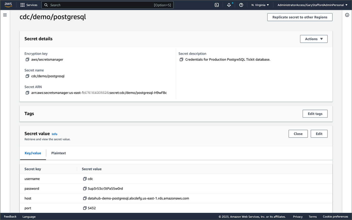
For self-managed Kafka Connect, I prefer Jeremy Custenborder’s kafka-config-provider-aws plugin. This plugin provides integration with AWS Secrets Manager. A complete list of Jeremy’s providers can be found on GitHub. Below is a snippet of the Secrets Manager configuration from the connect-distributed.properties files, which is read by Apache Kafka Connect at startup.
https://garystafford.medium.com/media/db6ff589c946fcd014546c56d0255fe5
Apache Avro
The message in the Kafka topic and corresponding objects in Amazon S3 will be stored in Apache Avro format by the CDC process. The Apache Avro documentation states, “Apache Avro is the leading serialization format for record data, and the first choice for streaming data pipelines.” Avro provides rich data structures and a compact, fast, binary data format.
Again, according to the Apache Avro documentation, “Avro relies on schemas. When Avro data is read, the schema used when writing it is always present. This permits each datum to be written with no per-value overheads, making serialization both fast and small. This also facilitates use with dynamic, scripting languages, since data, together with its schema, is fully self-describing.” When Avro data is stored in a file, its schema can be stored with it so any program may process files later.
Alternatively, the schema can be stored separately in a schema registry. According to Apicurio Registry, “in the messaging and event streaming world, data that are published to topics and queues often must be serialized or validated using a Schema (e.g. Apache Avro, JSON Schema, or Google protocol buffers). Schemas can be packaged in each application, but it is often a better architectural pattern to instead register them in an external system [schema registry] and then referenced from each application.”
Schema Registry
Several leading open-source and commercial schema registries exist, including Confluent Schema Registry, AWS Glue Schema Registry, and Red Hat’s open-source Apicurio Registry. In this post, we use a self-managed version of Apicurio Registry running on Amazon EKS. You can relatively easily substitute AWS Glue Schema Registry if you prefer a fully-managed AWS service.
Apicurio Registry
According to the documentation, Apicurio Registry supports adding, removing, and updating OpenAPI, AsyncAPI, GraphQL, Apache Avro, Google protocol buffers, JSON Schema, Kafka Connect schema, WSDL, and XML Schema (XSD) artifact types. Furthermore, content evolution can be controlled by enabling content rules, including validity and compatibility. Lastly, the registry can be configured to store data in various backend storage systems depending on the use case, including Kafka (e.g., Amazon MSK), PostgreSQL (e.g., Amazon RDS), and Infinispan (embedded).
Data Lake Table Formats
Three leading open-source, transactional data lake storage frameworks enable building data lake and data lakehouse architectures: Apache Iceberg, Linux Foundation Delta Lake, and Apache Hudi. They offer comparable features, such as ACID-compliant transactional guarantees, time travel, rollback, and schema evolution. Using any of these three data lake table formats will allow us to store and perform analytics on the latest version of the data in the data lake originating from the three Amazon RDS databases.
Apache Hudi
According to the Apache Hudi documentation, “Apache Hudi is a transactional data lake platform that brings database and data warehouse capabilities to the data lake.” The specifics of how the data is laid out as files in your data lake depends on the Hudi table type you choose, either Copy on Write (CoW) or Merge On Read (MoR).
Like Apache Iceberg and Delta Lake, Apache Hudi is partially supported by AWS’s Analytics services, including AWS Glue, Amazon EMR, Amazon Athena, Amazon Redshift Spectrum, and AWS Lake Formation. In general, CoW has broader support on AWS than MoR. It is important to understand the limitations of Apache Hudi with each AWS analytics service before choosing a table format.
If you are looking for a fully-managed Cloud data lake service built on Hudi, I recommend Onehouse. Born from the roots of Apache Hudi and founded by its original creator, Vinoth Chandar (PMC chair of the Apache Hudi project), the Onehouse product and its services leverage OSS Hudi to offer a data lake platform similar to what companies like Uber have built.
Hudi DeltaStreamer
Hudi also offers DeltaStreamer (aka HoodieDeltaStreamer) for streaming ingestion of CDC data. DeltaStreamer can be run once or continuously, using Apache Spark, similar to an Apache Spark Structured Streaming job, to capture changes to the raw CDC data and write that data to a different part of our data lake.
DeltaStreamer also works with Amazon S3 Event Notifications instead of running continuously. According to DeltaStreamer’s documentation, Amazon S3 object storage provides an event notification service to post notifications when certain events happen in your S3 bucket. AWS will put these events in Amazon Simple Queue Service (Amazon SQS). Apache Hudi provides an S3EventsSource that can read from Amazon SQS to trigger and process new or changed data as soon as it is available on Amazon S3.
Sample Data for the Data Lake
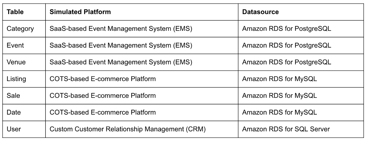
The data used in this post is from the TICKIT sample database. The TICKIT database represents the backend data store for a platform that brings buyers and sellers of tickets to entertainment events together. It was initially designed to demonstrate Amazon Redshift. The TICKIT database is a small database with approximately 425K rows of data across seven tables: Category, Event, Venue, User, Listing, Sale, and Date.
A data lake most often contains data from multiple sources, each with different storage formats, protocols, and connection methods. To simulate these data sources, I have separated the TICKIT database tables to represent three typical enterprise systems, including a commercial off-the-shelf (COTS) E-commerce platform, a custom Customer Relationship Management (CRM) platform, and a SaaS-based Event Management System (EMS). Each simulated system uses a different Amazon RDS database engine, including MySQL, PostgreSQL, and SQL Server.
Enabling CDC for Amazon RDS
To use Debezium for CDC with Amazon RDS databases, minor changes to the default database configuration for each database engine are required.
CDC for PostgreSQL
Debezium has detailed instructions regarding configuring CDC for Amazon RDS for PostgreSQL. Database parameters specify how the database is configured. According to the Debezium documentation, for PostgreSQL, set the instance parameter rds.logical_replication to 1 and verify that the wal_level parameter is set to logical. It is automatically changed when the rds.logical_replication parameter is set to 1. This parameter is adjusted using an Amazon RDS custom parameter group. According to the AWS documentation, “with Amazon RDS, you manage database configuration by associating your DB instances and Multi-AZ DB clusters with parameter groups. Amazon RDS defines parameter groups with default settings. You can also define your own parameter groups with customized settings.”

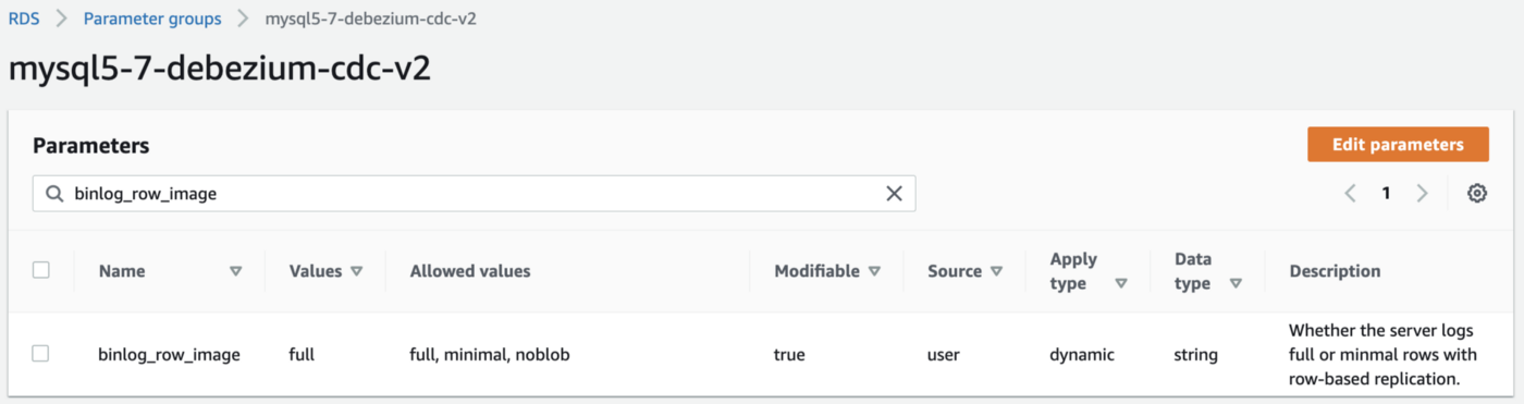
CDC for MySQL
Similarly, Debezium has detailed instructions regarding configuring CDC for MySQL. Like PostgreSQL, MySQL requires a custom DB parameter group.


CDC for SQL Server
Lastly, Debezium has detailed instructions for configuring CDC with Microsoft SQL Server. Enabling CDC requires enabling CDC on the SQL Server database and table(s) and creating a new filegroup and associated file. Debezium recommends locating change tables in a different filegroup than you use for source tables. CDC is only supported with Microsoft SQL Server Standard Edition and higher; Express and Web Editions are not supported.
Kafka Connect Source Connectors
There is a Kafka Connect source connector for each of the three Amazon RDS databases, all of which use Debezium. CDC is performed, moving changes from the three databases into separate Kafka topics in Apache Avro format using the source connectors. The connector configuration is nearly identical whether you are using Amazon MSK Connect or a self-managed version of Kafka Connect.
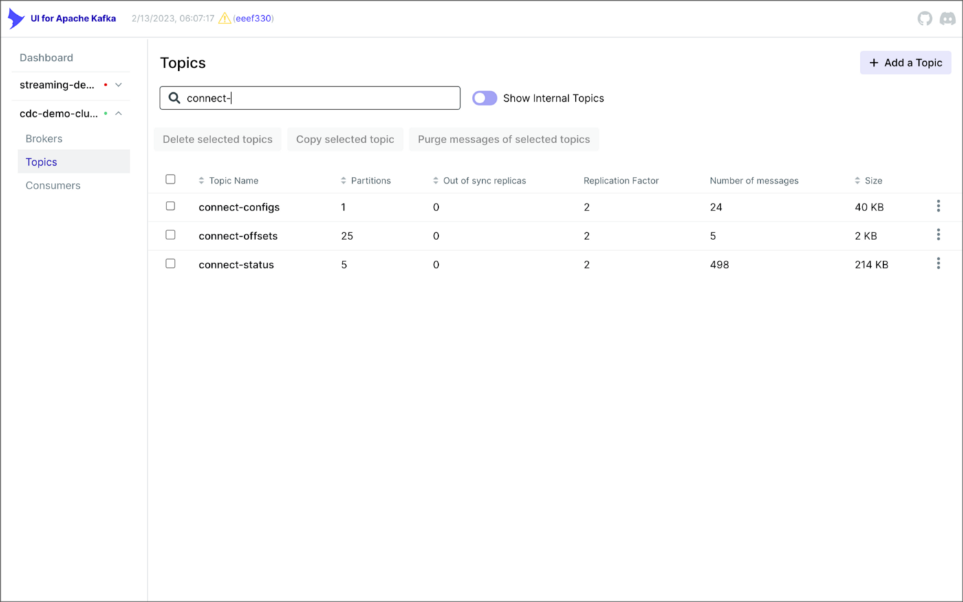
As shown above, I am using the UI for Apache Kafka by Provectus, self-managed on Amazon EKS, in this post.
PostgreSQL Source Connector
The source_connector_postgres_kafka_avro_tickit source connector captures all changes to the three tables in the Amazon RDS for PostgreSQL ticket database’s ems schema: category, event, and venue. These changes are written to three corresponding Kafka topics as Avro-format messages: tickit.ems.category, tickit.ems.event, and tickit.ems.venue. The messages are transformed by the connector using Debezium’s unwrap transform. Schemas for the messages are written to Apicurio Registry.
MySQL Source Connector
The source_connector_mysql_kafka_avro_tickit source connector captures all changes to the three tables in the Amazon RDS for PostgreSQL ecomm database: date, listing, and sale. These changes are written to three corresponding Kafka topics as Avro-format messages: tickit.ecomm.date, tickit.ecomm.listing, and tickit.ecomm.sale.
SQL Server Source Connector
Lastly, the source_connector_mssql_kafka_avro_tickit source connector captures all changes to the single user table in the Amazon RDS for SQL Server ticket database’s crm schema. These changes are written to a corresponding Kafka topic as Avro-format messages: tickit.crm.user.
If using a self-managed version of Kafka Connect, we can deploy, manage, and monitor the source and sink connectors using Kafka Connect’s RESTful API (Connect API).

Once the three source connectors are running, we should see seven new Kafka topics corresponding to the seven TICKIT database tables from the three Amazon RDS database sources. There will be approximately 425K messages consuming 147 MB of space in Avro’s binary format.
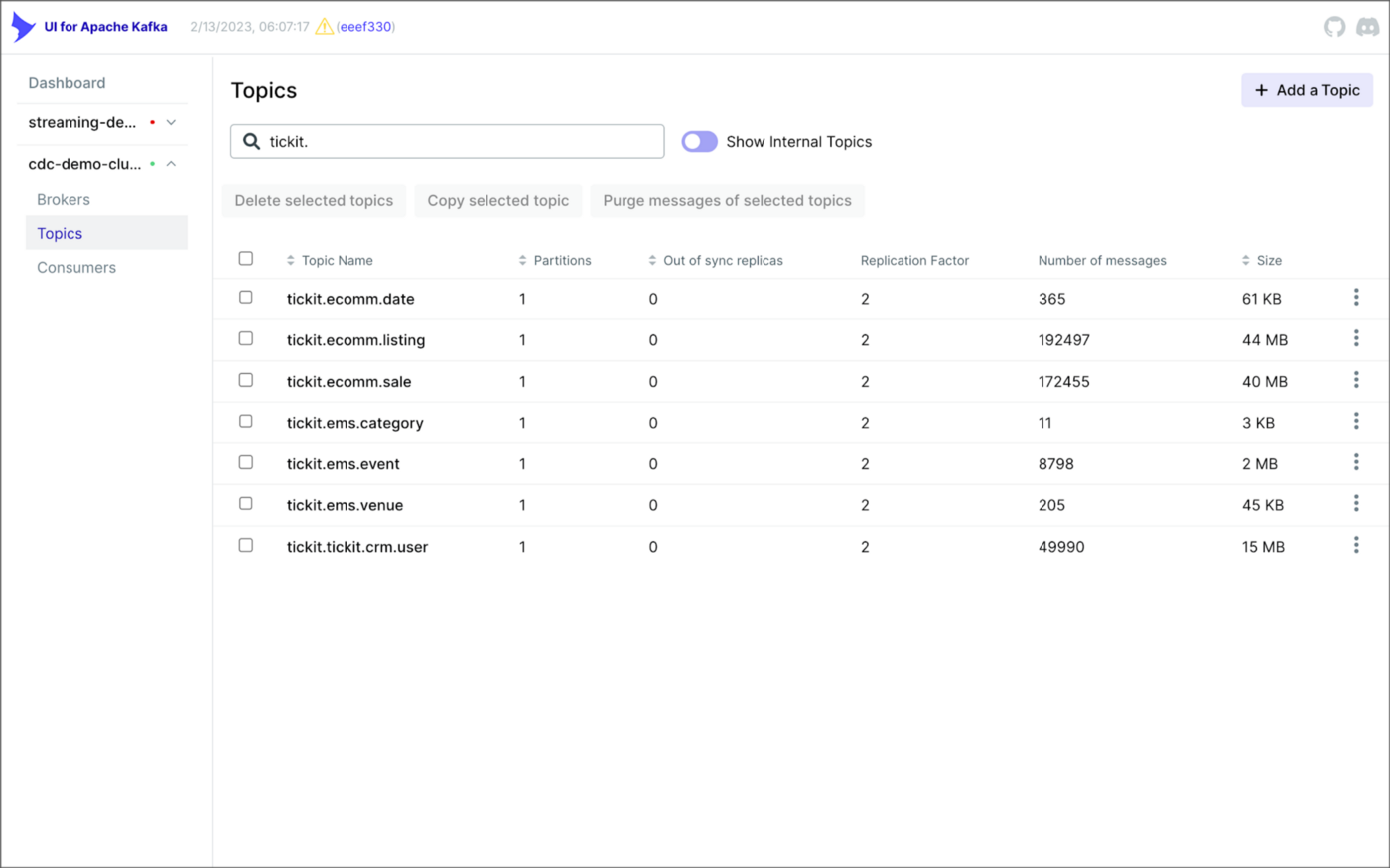
Avro’s binary format and the use of a separate schema ensure the messages consume minimal Kafka storage space. For example, the average message Value (payload) size in the tickit.ecomm.sale topic is a minuscule 98 Bytes. Resource management is critical when you are dealing with hundreds of millions or often billions of daily Kafka messages as a result of the CDC process.

From within the Apicurio Registry UI, we should now see Value schema artifacts for each of the seven Kafka topics.
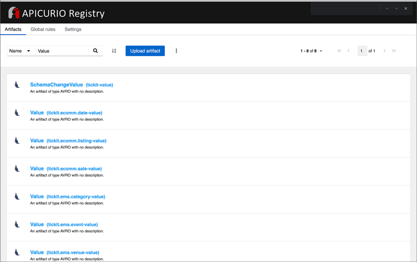
Also from within the Apicurio Registry UI, we can examine details of individual Value schema artifacts.

Kafka Connect Sink Connector
In addition to the three source connectors, there is a single Kafka Connect sink connector, sink_connector_kafka_s3_avro_tickit. The sink connector copies messages from the seven Kafka topics, all prefixed with tickit, to the Bronze area of our Amazon S3-based data lake.

The connector uses Confluent’s S3 Sink Connector (S3SinkConnector). Like Kafka, the connector writes all changes to Amazon S3 in Apache Avro format, with the schemas already stored in Apicurio Registry.
Once the sink connector and the three source connectors are running with Kafka Connect, we should see a series of seven subdirectories within the Bronze area of the data lake.

Confluent offers a choice of data partitioning strategies. The sink connector we have deployed uses the Daily Partitioner. According to the documentation, the io.confluent.connect.storage.partitioner.DailyPartitioner is equivalent to the TimeBasedPartitioner with path.format='year'=YYYY/'month'=MM/'day'=dd and partition.duration.ms=86400000 (one day for one S3 object in each daily directory). Below is an example of Avro files (S3 objects) containing changes to the sale table. The objects are partitioned by the year, month, and day they were written to the S3 bucket.

Message Transformation
Previously, while discussing the Kafka Connect source connectors, I mentioned that the connector transforms the messages using the unwrap transform. By default, the changes picked up by Debezium during the CDC process contain several additional Debezium-related fields of data. An example of an untransformed message generated by Debezium from the PostgreSQL sale table is shown below.
When the PostgreSQL connector first connects to a particular PostgreSQL database, it starts by performing a consistent snapshot of each database schema. All existing records are captured. Unlike an UPDATE ("op" : "u") or a DELETE ("op" : "d"), these initial snapshot messages, like the one shown below, represent a READ operation ("op" : "r"). As a result, there is no before data only after.
According to Debezium’s documentation, “Debezium provides a single message transformation [SMT] that crosses the bridge between the complex and simple formats, the UnwrapFromEnvelope SMT.” Below, we see the results of Debezium’s unwrap transform of the same message. The unwrap transform flattens the nested JSON structure of the original message, adds the __deleted field, and includes fields based on the list included in the source connector’s configuration. These fields are prefixed with a double underscore (e.g., __table).
In the next section, we examine Apache Hudi will manage the data lake. An example of the same message, managed with Hudi, is shown below. Note the five additional Hudi data fields, prefixed with _hoodie_.
Apache Hudi
With database changes flowing into the Bronze area of our data lake, we are ready to use Apache Hudi to provide data lake capabilities such as ACID transactional guarantees, time travel, rollback, and schema evolution. Using Hudi allows us to store and perform analytics on a specific time-bound version of the data in the data lake. Without Hudi, a query for a single row of data could return multiple results, such as an initial CREATE record, multiple UPDATE records, and a DELETE record.
DeltaStreamer
Using Hudi’s DeltaStreamer, we will continuously stream changes from the Bronze area of the data lake to a Silver area, which Hudi manages. We will run DeltaStreamer continuously, similar to an Apache Spark Structured Streaming job, using Apache Spark on Amazon EMR. Running DeltaStreamer requires using a spark-submit command that references a series of configuration files. There is a common base set of configuration items and a group of configuration items specific to each database table. Below, we see the base configuration, base.properties.
The base configuration is referenced by each of the table-specific configuration files. For example, below, we see the tickit.ecomm.sale.properties configuration file for DeltaStreamer.
To run DeltaStreamer, you can submit an EMR Step or use EMR’s master node to run a spark-submit command on the cluster. Below, we see an example of the DeltaStreamer spark-submit command using the Merge on Read (MoR) Hudi table type.
Next, we see the same example of the DeltaStreamer spark-submit command using the Copy on Write (CoW) Hudi table type.
For this post’s demonstration, we will run a single-table DeltaStreamer Spark job, with one process for each table using CoW. Alternately, Hudi offers HoodieMultiTableDeltaStreamer, a wrapper on top of HoodieDeltaStreamer, which enables the ingestion of multiple tables at a single time into Hudi datasets. Currently, HoodieMultiTableDeltaStreamer only supports sequential processing of tables to be ingested and COPY_ON_WRITE storage type.
Below, we see an example of three DeltaStreamer Spark jobs running continuously for the date, listing, and sale tables.

Once DeltaStreamer is up and running, we should see a series of subdirectories within the Silver area of the data lake, all managed by Apache Hudi.
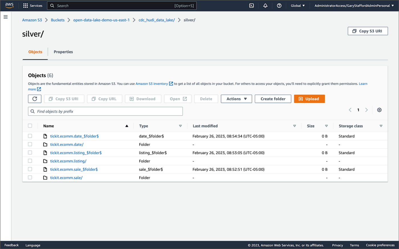
Within each subdirectory, partitioned by the table name, is a series of Apache Parquet files, along with other Apache Hudi-specific files. The specific folder structure and files depend on MoR or Cow.

AWS Glue Data Catalog
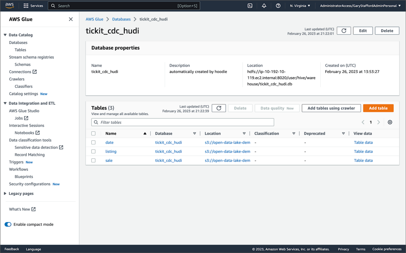
For this post, we are using an AWS Glue Data Catalog, an Apache Hive-compatible metastore, to persist technical metadata stored in the Silver area of the data lake, managed by Apache Hudi. The AWS Glue Data Catalog database, tickit_cdc_hudi, will be automatically created the first time DeltaStreamer runs.
Using DeltaStreamer with the table type of MERGE_ON_READ, there would be two tables in the AWS Glue Data Catalog database for each original table. According to Amazon’s EMR documentation, “Merge on Read (MoR) — Data is stored using a combination of columnar (Parquet) and row-based (Avro) formats. Updates are logged to row-based delta files and are compacted as needed to create new versions of the columnar files.” Hudi creates two tables in the Hive metastore for MoR, a table with the name that you specified, which is a read-optimized view (appended with _ro), and a table with the same name appended with _rt, which is a real-time view. You can query both tables.
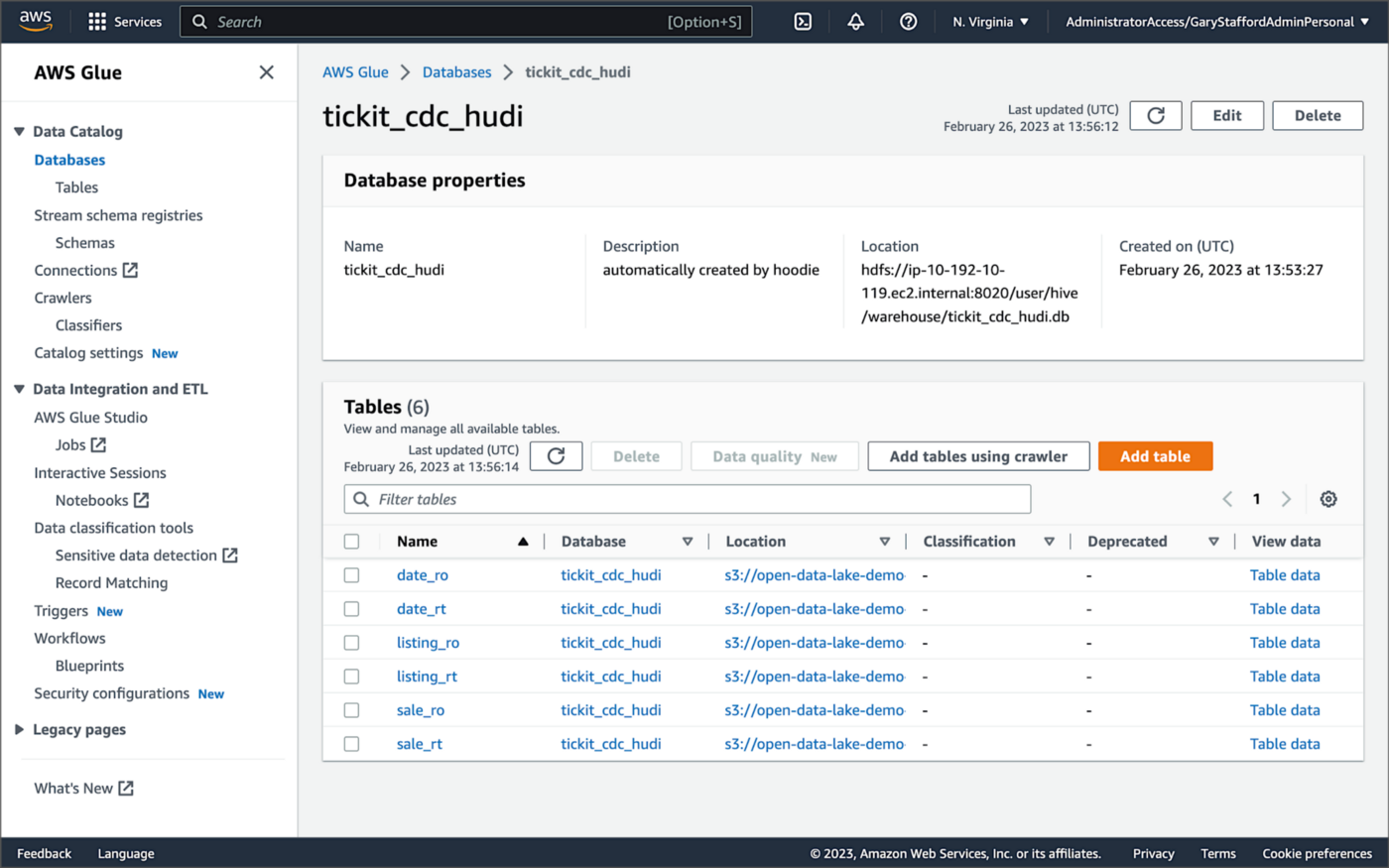
According to Amazon’s EMR documentation, “Copy on Write (CoW) — Data is stored in a columnar format (Parquet), and each update creates a new version of files during a write. CoW is the default storage type.” Using COPY_ON_WRITE with DeltaStreamer, there is only a single Hudi table in the AWS Glue Data Catalog database for each corresponding database table.
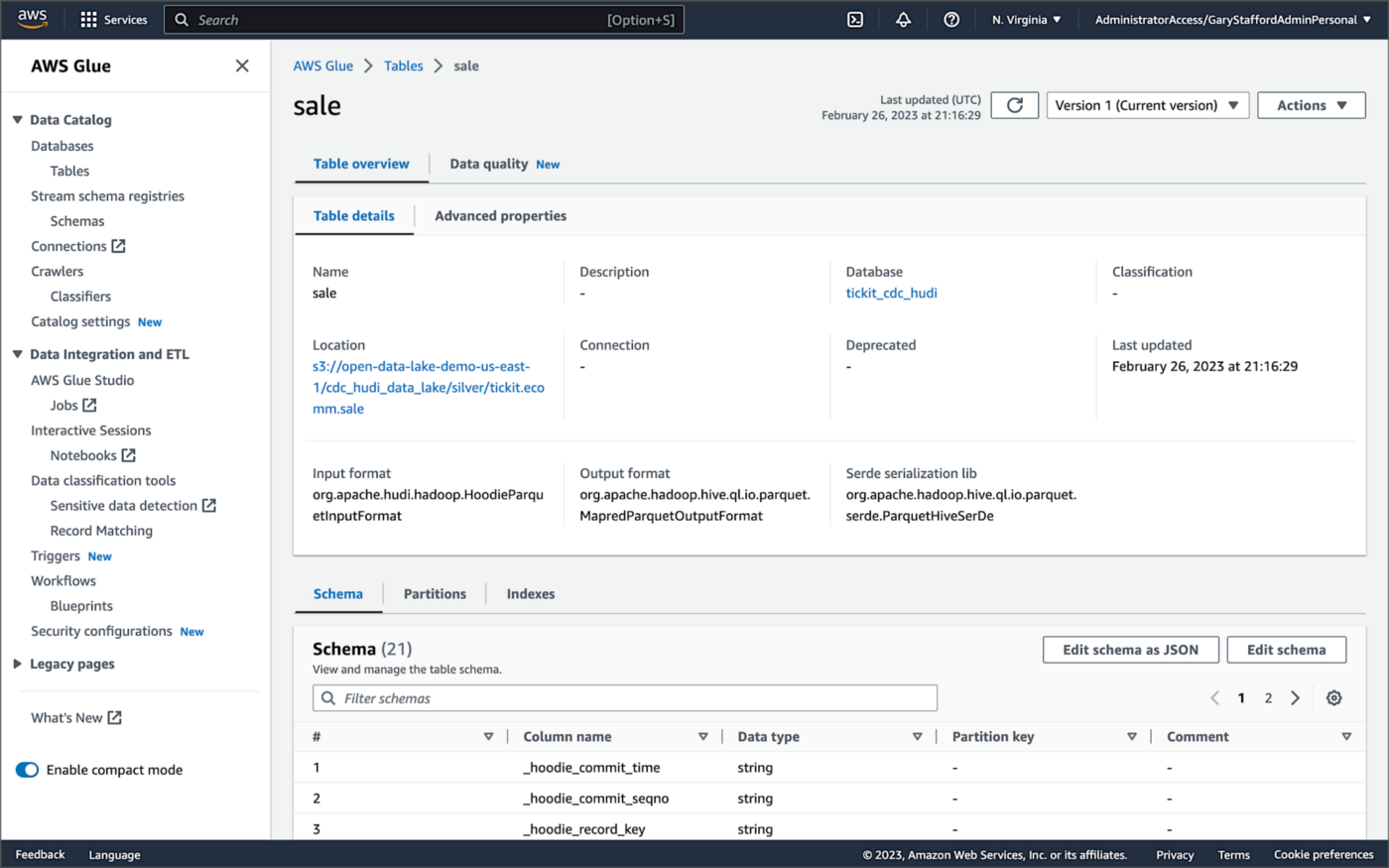
Examining an individual table in the AWS Glue Data Catalog database, we can see details like the table schema, location of underlying data in S3, input/output formats, Serde serialization library, and table partitions.
Database Changes and Data Lake
We are using Kafka Connect, Apache Hudi, and Hudi’s DeltaStreamer to maintain data parity between our databases and the data lake. Let’s look at an example of how a simple data change is propagated from a database to Kafka, then to the Bronze area of the data lake, and finally to the Hudi-managed Silver area of the data lake, written using the CoW table format.
First, we will make a simple update to a single record in the MySQL database’s sale table with the salesid = 200.
Almost immediately, we can see the change picked up by the Kafka Connect Debezium MySQL source connector.

Almost immediately, in the Bronze area of the data lake, we can see we have a new Avro-formatted file (S3 object) containing the updated record in the partitioned sale subdirectory.

If we examine the new object in the Bronze area of the data lake, we will see a row representing the updated record with the salesid = 200. Note how the operation is now an UPDATE versus a READ ("op" : "u").
Next, in the corresponding Silver area of the data lake, managed by Hudi, we should also see a new Parquet file that contains a record of the change. In this example, the file was written approximately 26 seconds after the original change to the database. This is the end-to-end time from database change to when the updated data is queryable in the data lake.
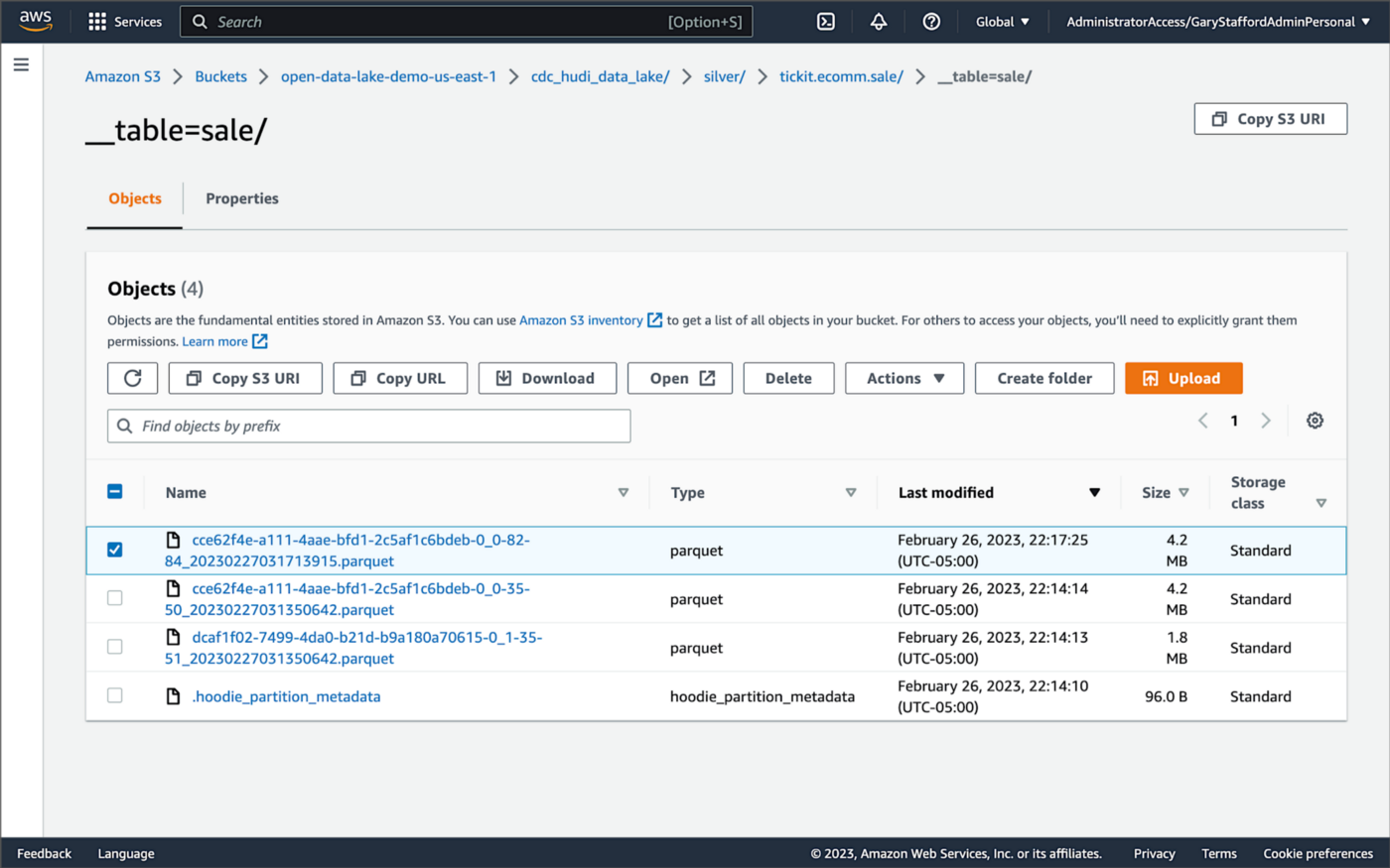
Similarly, if we examine the new object in the Silver area of the data lake, we will see a row representing the updated record with the salesid = 200. The record was committed approximately 15 seconds after the original database change.
Querying Hudi Tables with Amazon EMR
Using an EMR Notebook, we can query the updated database record stored in Amazon S3 using Hudi’s CoW table format. First, running a simple Spark SQL query for the record with salesid = 200, returns the latest record, reflecting the changes as indicated by the UPDATE operation value (u) and the _hoodie_commit_time = 2023-02-27 03:17:13.915 UTC.

Hudi Time Travel Query
We can also run a Hudi Time Travel Query, with an as.of.instance set to some arbitrary point in the future. Again, the latest record is returned, reflecting the changes as indicated by the UPDATE operation value (u) and the _hoodie_commit_time = 2023-02-27 03:17:13.915 UTC.

We can run the same Hudi Time Travel Query with an as.of.instance set to on or after the original records were written by DeltaStreamer (_hoodie_commit_time = 2023-02-27 03:13:50.642), but some arbitrary time before the updated record was written (_hoodie_commit_time = 2023-02-27 03:17:13.915). This time, the original record is returned as indicated by the READ operation value (r) and the _hoodie_commit_time = 2023-02-27 03:13:50.642. This is one of the strengths of Apache Hudi, the ability to query data in the present or at any point in the past.

Hudi Point in Time Query
We can also run a Hudi Point in Time Query, with a time range set from the beginning of time until some arbitrary point in the future. Again, the latest record is returned, reflecting the changes as indicated by the UPDATE operation value (u) and the _hoodie_commit_time = 2023-02-27 03:17:13.915.

We can run the same Hudi Point in Time Query but change the time range to two arbitrary time values, both before the updated record was written (_hoodie_commit_time = 2023-02-26 22:39:07.203). This time, the original record is returned as indicated by the READ operation value (r) and the _hoodie_commit_time of 2023-02-27 03:13:50.642. Again, this is one of the strengths of Apache Hudi, the ability to query data in the present or at any point in the past.

Querying Hudi Tables with Amazon Athena
We can also use Amazon Athena and run a SQL query against the AWS Glue Data Catalog database’s sale table to view the updated database record stored in Amazon S3 using Hudi’s CoW table format. The operation (op) column’s value now indicates an UPDATE (u).

How are Deletes Handled?
In this post’s architecture, deleted database records are signified with an operation ("op") field value of "d" for a DELETE and a __deleted field value of true.
https://itnext.io/media/f7c4ad62dcd45543fdf63834814a5aab
Back to our previous Jupyter notebook example, when rerunning the Spark SQL query, the latest record is returned, reflecting the changes as indicated by the DELETE operation value (d) and the _hoodie_commit_time = 2023-02-27 03:52:13.689.

Alternatively, we could use an additional Spark SQL filter statement to prevent deleted records from being returned (e.g., df.__op != "d").

Since we only did what is referred to as a soft delete in Hudi terminology, we can run a time travel query with an as.of.instance set to some arbitrary time before the deleted record was written (_hoodie_commit_time = 2023-02-27 03:52:13.689). This time, the original record is returned as indicated by the READ operation value (r) and the _hoodie_commit_time = 2023-02-27 03:13:50.642. We could also use a later as.of.instance to return the version of the record reflecting the the UPDATE operation value (u). This also applies to other query types such as point-in-time queries.

Conclusion
In this post, we learned how to build a near real-time transactional data lake on AWS using one possible architecture. The data lake was built using a combination of open source software (OSS) and fully-managed AWS services. Red Hat’s Debezium, Apache Kafka, and Kafka Connect were used for change data capture (CDC). In addition, Apache Spark, Apache Hudi, and Hudi’s DeltaStreamer were used to manage the data lake. To complete our architecture, we used several fully-managed AWS services, including Amazon RDS, Amazon MKS, Amazon EKS, AWS Glue, and Amazon EMR.
This blog represents my own viewpoints and not of my employer, Amazon Web Services (AWS). All product names, logos, and brands are the property of their respective owners.
The Art of Building Open Data Lakes with Apache Hudi, Kafka, Hive, and Debezium
Posted by Gary A. Stafford in Analytics, AWS, Big Data, Cloud, Python, Software Development, Technology Consulting on December 31, 2021
Build near real-time, open-source data lakes on AWS using a combination of Apache Kafka, Hudi, Spark, Hive, and Debezium
Introduction
In the following post, we will learn how to build a data lake on AWS using a combination of open-source software (OSS), including Red Hat’s Debezium, Apache Kafka, Kafka Connect, Apache Hive, Apache Spark, Apache Hudi, and Hudi DeltaStreamer. We will use fully-managed AWS services to host the datasource, the data lake, and the open-source tools. These services include Amazon RDS, MKS, EKS, EMR, and S3.

This post is an in-depth follow-up to the video demonstration, Building Open Data Lakes on AWS with Debezium and Apache Hudi.
Workflow
As shown in the architectural diagram above, these are the high-level steps in the demonstration’s workflow:
- Changes (inserts, updates, and deletes) are made to the datasource, a PostgreSQL database running on Amazon RDS;
- Kafka Connect Source Connector, utilizing Debezium and running on Amazon EKS (Kubernetes), continuously reads data from PostgreSQL WAL using Debezium;
- Source Connector creates and stores message schemas in Apicurio Registry, also running on Amazon EKS, in Avro format;
- Source Connector transforms and writes data in Apache Avro format to Apache Kafka, running on Amazon MSK;
- Kafka Connect Sink Connector, using Confluent S3 Sink Connector, reads messages from Kafka topics using schemas from Apicurio Registry;
- Sink Connector writes data to Amazon S3 in Apache Avro format;
- Apache Spark, using Hudi DeltaStreamer and running on Amazon EMR, reads message schemas from Apicurio Registry;
- DeltaStreamer reads raw Avro-format data from Amazon S3;
- DeltaStreamer writes data to Amazon S3 as both Copy on Write (CoW) and Merge on Read (MoR) table types;
- DeltaStreamer syncs Hudi tables and partitions to Apache Hive running on Amazon EMR;
- Queries are executed against Apache Hive Metastore or directly against Hudi tables using Apache Spark, with data returned from Hudi tables in Amazon S3;
The workflow described above actually contains two independent processes running simultaneously. Steps 2–6 represent the first process, the change data capture (CDC) process. Kafka Connect is used to continuously move changes from the database to Amazon S3. Steps 7–10 represent the second process, the data lake ingestion process. Hudi’s DeltaStreamer reads raw CDC data from Amazon S3 and writes the data back to another location in S3 (the data lake) in Apache Hudi table format. When combined, these processes can give us near real-time, incremental data ingestion of changes from the datasource to the Hudi-managed data lake.
Alternatives
This demonstration’s workflow is only one of many possible workflows to achieve similar outcomes. Alternatives include:
- Replace self-managed Kafka Connect with the fully-managed Amazon MSK Connect service.
- Exchange Amazon EMR for AWS Glue Jobs or AWS Glue Studio and the custom AWS Glue Connector for Apache Hudi to ingest data into Hudi tables.
- Replace Apache Hive with AWS Glue Data Catalog, a fully-managed Hive-compatible metastore.
- Replace Apicurio Registry with Confluent Schema Registry or AWS Glue Schema Registry.
- Exchange the Confluent S3 Sink Connector for the Kafka Connect Sink for Hudi, which could greatly simplify the workflow.
- Substitute
HoodieMultiTableDeltaStreamerfor theHoodieDeltaStreamerutility to quickly ingest multiple tables into Hudi. - Replace Hudi’s AvroDFSSource for the AvroKafkaSource to read directly from Kafka versus Amazon S3, or Hudi’s JdbcSource to read directly from the PostgreSQL database. Hudi has several datasource readers available. Be cognizant of authentication/authorization compatibility/limitations.
- Choose either or both Hudi’s Copy on Write (CoW) and Merge on Read (MoR) table types depending on your workload requirements.
Source Code
All source code for this post and the previous posts in this series are open-sourced and located on GitHub. The specific resources used in this post are found in the debezium_hudi_demo directory of the GitHub repository. There are also two copies of the Museum of Modern Art (MoMA) Collection dataset from Kaggle, specifically prepared for this post, located in the moma_data directory. One copy is a nearly full dataset, and the other is a smaller, cost-effective dev/test version.
Kafka Connect
In this demonstration, Kafka Connect runs on Kubernetes, hosted on the fully-managed Amazon Elastic Kubernetes Service (Amazon EKS). Kafka Connect runs the Source and Sink Connectors.
Source Connector
The Kafka Connect Source Connector, source_connector_moma_postgres_kafka.json, used in steps 2–4 of the workflow, utilizes Debezium to continuously read changes to an Amazon RDS for PostgreSQL database. The PostgreSQL database hosts the MoMA Collection in two tables: artists and artworks.
The Debezium Connector for PostgreSQL reads record-level insert, update, and delete entries from PostgreSQL’s write-ahead log (WAL). According to the PostgreSQL documentation, changes to data files must be written only after log records describing the changes have been flushed to permanent storage, thus the name, write-ahead log. The Source Connector then creates and stores Apache Avro message schemas in Apicurio Registry also running on Amazon EKS.


Finally, the Source Connector transforms and writes Avro format messages to Apache Kafka running on the fully-managed Amazon Managed Streaming for Apache Kafka (Amazon MSK). Assuming Kafka’s topic.creation.enable property is set to true, Kafka Connect will create any necessary Kafka topics, one per database table.
Below, we see an example of a Kafka message representing an insert of a record with the artist_id 1 in the MoMA Collection database’s artists table. The record was read from the PostgreSQL WAL, transformed, and written to a corresponding Kafka topic, using the Debezium Connector for PostgreSQL. The first version represents the raw data before being transformed by Debezium. Note that the type of operation (_op) indicates a read (r). Possible values include c for create (or insert), u for update, d for delete, and r for read (applies to snapshots).
The next version represents the same record after being transformed by Debezium using the event flattening single message transformation (unwrap SMT). The final message structure represents the schema stored in Apicurio Registry. The message structure is identical to the structure of the data written to Amazon S3 by the Sink Connector.
Sink Connector
The Kafka Connect Sink Connector, sink_connector_moma_kafka_s3.json, used in steps 5–6 of the workflow, implements the Confluent S3 Sink Connector. The Sink Connector reads the Avro-format messages from Kafka using the schemas stored in Apicurio Registry. It then writes the data to Amazon S3, also in Apache Avro format, based on the same schemas.
Running Kafka Connect
We first start Kafka Connect in the background to be the CDC process.
Then, deploy the Kafka Connect Source and Sink Connectors using Kafka Connect’s RESTful API. Using the API, we can also confirm the status of the Connectors.
To confirm the two Kafka topics, moma.public.artists and moma.public.artworks, were created and contain Avro messages, we can use Kafka’s command-line tools.
In the short video-only clip below, we see the process of deploying the Kafka Connect Source and Sink Connectors and confirming they are working as expected.
The Sink Connector writes data to Amazon S3 in batches of 10k messages or every 60 seconds (one-minute intervals). These settings are configurable and highly dependent on your requirements, including message volume, message velocity, real-time analytics requirements, and available compute resources.

Since we will not be querying this raw Avro-format CDC data in Amazon S3 directly, there is no need to catalog this data in Apache Hive or AWS Glue Data Catalog, a fully-managed Hive-compatible metastore.
Apache Hudi
According to the overview, Apache Hudi (pronounced “hoodie”) is the next-generation streaming data lake platform. Apache Hudi brings core warehouse and database functionality to data lakes. Hudi provides tables, transactions, efficient upserts and deletes, advanced indexes, streaming ingestion services, data clustering, compaction optimizations, and concurrency, all while keeping data in open source file formats.
Without Hudi or an equivalent open-source data lake table format such as Apache Iceberg or Databrick’s Delta Lake, most data lakes are just of bunch of unmanaged flat files. Amazon S3 cannot natively maintain the latest view of the data, to the surprise of many who are more familiar with OLTP-style databases or OLAP-style data warehouses.
DeltaStreamer
DeltaStreamer, aka the HoodieDeltaStreamer utility (part of the hudi-utilities-bundle), used in steps 7–10 of the workflow, provides the way to perform streaming ingestion of data from different sources such as Distributed File System (DFS) and Apache Kafka.
Optionally, HoodieMultiTableDeltaStreamer, a wrapper on top of HoodieDeltaStreamer, ingests multiple tables in a single Spark job, into Hudi datasets. Currently, it only supports sequential processing of tables to be ingested and Copy on Write table type.
We are using HoodieDeltaStreamer to write to both Merge on Read (MoR) and Copy on Write (CoW) table types for demonstration purposes only. The MoR table type is a superset of the CoW table type, which stores data using a combination of columnar-based (e.g., Apache Parquet) plus row-based (e.g., Apache Avro) file formats. Updates are logged to delta files and later compacted to produce new versions of columnar files synchronously or asynchronously. Again, the choice of table types depends on your requirements.

Amazon EMR
For this demonstration, I’ve used the recently released Amazon EMR version 6.5.0 configured with Apache Spark 3.1.2 and Apache Hive 3.1.2. EMR 6.5.0 runs Scala version 2.12.10, Python 3.7.10, and OpenJDK Corretto-8.312. I have included the AWS CloudFormation template and parameters file used to create the EMR cluster, on GitHub.

When choosing Apache Spark, Apache Hive, or Presto on EMR 6.5.0, Apache Hudi release 0.9.0 is automatically installed.

DeltaStreamer Configuration
Below, we see the DeltaStreamer properties file, deltastreamer_artists_apicurio_mor.properties. This properties file is referenced by the Spark job that runs DeltaStreamer, shown next. The file contains properties related to the datasource, the data sink, and Apache Hive. The source of the data for DeltaStreamer is the CDC data written to Amazon S3. In this case, the datasource is the objects located in the /topics/moma.public.artworks/partition=0/ S3 object prefix. The data sink is a Hudi MoR table type in Amazon S3. DeltaStreamer will write Parquet data, partitioned by the artist’s nationality, to the /moma_mor/artists/ S3 object prefix. Lastly, DeltaStreamer will sync all tables and table partitions to Apache Hive, including creating the Hive databases and tables if they do not already exist.
Below, we see the equivalent DeltaStreamer properties file for the MoMA artworks, deltastreamer_artworks_apicurio_mor.properties. There are also comparable DeltaStreamer property files for the Hudi CoW tables on GitHub.
All DeltaStreamer property files reference Apicurio Registry for the location of the Avro schemas. The schemas are used by both the Kafka Avro-format messages and the CDC-created Avro-format files in Amazon S3. Due to DeltaStreamer’s coupling with Confluent Schema Registry, as opposed to other registries, we must use Apicurio Registry’s Confluent Schema Registry API (Version 6) compatibility API endpoints (e.g., /apis/ccompat/v6/subjects/moma.public.artists-value/versions/latest) when using the org.apache.hudi.utilities.schema.SchemaRegistryProvider datasource option with DeltaStreamer. According to Apicurio, to provide compatibility with Confluent SerDes (Serializer/Deserializer) and other clients, Apicurio Registry implements the API defined by the Confluent Schema Registry.

Running DeltaStreamer
The properties files are loaded by Spark jobs that call the DeltaStreamer library, using spark-submit. Below, we see an example Spark job that calls the DeltaStreamer class. DeltaStreamer reads the raw Avro-format CDC data from S3 and writes the data using the Hudi MoR table type into the /moma_mor/artists/ S3 object prefix. In this Spark particular job, we are using the continuous option. DeltaStreamer runs in continuous mode using this option, running source-fetch, transform, and write in a loop. We are also using the UPSERT write operation (op). Operation options include UPSERT, INSERT, and BULK_INSERT. This set of options is ideal for inserting ongoing changes to CDC data into Hudi tables. You can run jobs in the foreground or background on EMR’s Master Node or as EMR Steps from the Amazon EMR console.
Below, we see another example DeltaStreamer Spark job that reads the raw Avro-format CDC data from S3 and writes the data using the MoR table type into the /moma_mor/artworks/ S3 object prefix. This example uses the BULK_INSERT write operation (op) and the filter-dupes option. The filter-dupes option ensures that should duplicate records from the source are dropped/filtered out before INSERT or BULK_INSERT. This set of options is ideal for the initial bulk inserting of existing data into Hudi tables. The job runs one time and completes, unlike the previous example that ran continuously.
Syncing with Hive
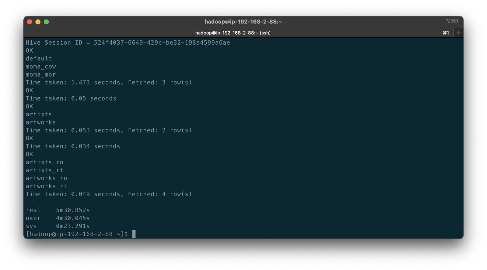
The following abridged, video-only clip demonstrates the differences between the Hudi CoW and MoR table types with respect to Apache Hive. In the video, we run the deltastreamer_jobs_bulk_bkgd.sh script, included on GitHub. This script runs four different Apache Spark jobs, using Hudi DeltaStreamer to bulk-ingest all the artists and artworks CDC data from Amazon S3 into both Hudi CoW and MoR table types. Once the four Spark jobs are complete, the script queries Apache Hive and displays the new Hive databases and database tables created by DeltaStreamer.
In both the video above and terminal screengrab below, note the difference in the tables created within the two Hive databases, the Hudi CoW table type (moma_cow) and the MoR table type (moma_mor). The MoR table type creates both a read-optimized table (_ro) as well as a real-time table (_rt) for each datasource (e.g., artists_ro and artists_rt).
According to documentation, Hudi creates two tables in the Hive metastore for the MoR table type. The first, a table which is a read-optimized view appended with _ro and the second, a table with the same name appended with _rt which is a real-time view. According to Hudi, the read-optimized view exposes columnar Parquet while the real-time view exposes columnar Parquet and/or row-based logs; you can query both tables. The CoW table type creates a single table without a suffix for each datasource (e.g., artists). Below, we see the Hive table structure for the artists_rt table, created by DeltaStreamer, using SHOW CREATE TABLE moma_mor.artists_rt;.
Having run the demonstration’s deltastreamer_jobs_bulk_bkgd.sh script, the resulting object structure in the Hudi-managed section of the Amazon S3 bucket looks as follows.

Below is an example of Hudi files created in the /moma/artists_cow/ S3 object prefix. When using data lake table formats like Hudi, given its specialized directory structure and the high number of objects, interactions with the data should be abstracted through Hudi’s programming interfaces. Generally speaking, you do not interact directly with the objects in a data lake.
Hudi CLI
Optionally, we can inspect the Hudi tables using the Hudi CLI (hudi-cli). The CLI offers an extensive list of available commands. Using the CLI, we can inspect the Hudi tables and their schemas, and review operational statistics like write amplification (the number of bytes written for 1 byte of incoming data), commits, and compactions.
The following short video-only clip shows the use of the Hudi CLI, running on the Amazon EMR Master Node, to inspect the Hudi tables in S3.
Hudi Data Structure
Recall the sample Kafka message we saw earlier in the post representing an insert of an artist record with the artist_id 1. Below, we see what the same record looks like after being ingested by Hudi DeltaStreamer. Note the five additional fields added by Hudi with the _hoodie_ prefix.
Querying Hudi-managed Data
With the initial data ingestion complete and the CDC and DeltaStreamer processes monitoring for future changes, we can query the resulting data stored in Hudi tables. First, we will make some changes to the PostgreSQL MoMA Collection database to see how Hudi manages the data mutations. We could also make changes directly to the Hudi tables using Hive, Spark, or Presto. However, that would cause our datasource to be out of sync with the Hudi tables, potentially negating the entire CDC process. When developing a data lake, this is a critically important consideration — how changes are introduced to Hudi tables, especially when CDC is involved, and whether data continuity between datasources and the data lake is essential.
For the demonstration, I have made a series of arbitrary updates to a piece of artwork in the MoMA Collection database, ‘Picador (La Pique)’ by Pablo Picasso.
Below, note the last four objects shown in S3. Judging by the file names and dates, we can see that the CDC process, using Kafka Connect, has picked up the four updates I made to the record in the database. The Source Connector first wrote the changes to Kafka. The Sink Connector then read those Kafka messages and wrote the data to Amazon S3 in Avro format, as shown below.

Looking again at S3, we can also observe that DeltaStreamer picked up the new CDC objects in Amazon S3 and wrote them to both the Hudi CoW and MoR tables. Note the file types shown below. Given Hudi’s MoR table type structure, Hudi first logged the changes to row-based delta files and later compacted them to produce a new version of the columnar-format Parquet file.

Querying Results from Apache Hive
There are several ways to query Hudi-managed data in S3. In this demonstration, they include against Apache Hive using the hive client from the command line, against Hive using Spark, and against the Hudi tables also using Spark. We could also install Presto on EMR to query the Hudi data directly or via Hive.
Querying the real-time artwork_rt table in Hive after we make each database change, we can observe the data in Hudi reflects the updates. Note that the value of the _hoodie_file_name field for the first three updates is a Hudi delta log file, while the value for the last update is a Parquet file. The Parquet file signifies compaction occurred between the fourth update was made, and the time the Hive query was executed. Lastly, note the type of operation (_op) indicates an update change (u) for all records.

Once all fours database updates are complete and compaction has occurred, we should observe identical results from all Hive tables. Below, note the _hoodie_file_name field for all three tables is a Parquet file. Logically, the Parquet file for the MoR read-optimized and real-time Hive tables is the same.

Had we queried the data previous to compaction, the results would have differed. Below we have three queries. I further updated the artwork record, changing the date field from 1959 to 1960. The read-optimized MoR table, artworks_ro, still reflects the original date value, 1959, before the update and prior to compaction. The real-time table,artworks_rt , reflects the latest update to the date field, 1960. Note that the value of the _hoodie_file_name field for the read-optimized table is a Parquet file, while the value for the real-time table (artworks_rt), the third and final query, is a delta log file. The delta log allows the real-time table to display the most current state of the data in Hudi.

Below are a few useful Hive commands to query the changes in Hudi.
Deletes with Hudi
In addition to inserts and updates (upserts), Apache Hudi can manage deletes. Hudi supports implementing two types of deletes on data stored in Hudi tables: soft deletes and hard deletes. Given this demonstration’s specific configuration for CDC and DeltaStreamer, we will use soft deletes. Soft deletes retain the record key and nullify the other field’s values. Hard deletes, a stronger form of deletion, physically remove any record trace from the Hudi table.
Below, we see the CDC record for the artist with artist_id 441. The event flattening single message transformation (SMT), used by the Debezium-based Kafka Connect Source Connector, adds the __deleted field with a value of true and nullifies all fields except the record’s key, artist_id, which is required.
Below, we see the same delete record for the artist with artist_id 441 in the Hudi MoR table. All the null fields have been removed.
Below, we see how the deleted record appears in the three Hive CoW and MoR artwork tables. Note the query results from the read-optimized MoR table, artworks_ro, contains two records — the original record (r) and the deleted record (d). The data is partitioned by nationality, and since the record was deleted, the nationality field is changed to null. In S3, Hudi represents this partition as nationality=default. The record now exists in two different Parquet files, within two separate partitions, something to be aware of when querying the read-optimized MoR table.

Time Travel
According to the documentation, Hudi has supported time travel queries since version 0.9.0. With time travel, you can query the previous state of your data. Time travel is particularly useful for use cases, including rollbacks, debugging, and audit history.
To demonstrate time travel queries in Hudi, we start by making some additional changes to the source database. For this demonstration, I made a series of five updates and finally a delete to the artist record with artist_id 299 in the PostgreSQL database over a few-hour period.
Once the CDC and DeltaStreamer ingestion processes are complete, we can use Hudi’s time travel query capability to view the state of data in Hudi at different points in time (instants). To do so, we need to provide an as.an.instant date/time value to Spark (see line 21 below).
Based on the time period in which I made the five updates and the delete, I have chosen six instants during that period where I want to examine the state of the record. Below is an example of the PySpark code from a Jupyter Notebook used to perform the six time travel queries against the Hudi MoR artist’s table.
Below, we see the results of the time travel queries. At each instant, we can observe the mutating state of the data in the Hudi MoR Artist’s table, including the initial bulk insert of the existing snapshot of data (r) and the delete record (d). Since the delete made in the PostgreSQL database was recorded as a soft delete in Hudi, as opposed to a hard delete, we are still able to retrieve the record at any instant.
In addition to time travel queries, Hudi also offers incremental queries and point in time queries.
Conclusion
Although this post only scratches the surface of the capabilities of Debezium and Hudi, you can see the power of CDC using Kafka Connect and Debezium, combined with Hudi, to build and manage open data lakes on AWS.
This blog represents my own viewpoints and not of my employer, Amazon Web Services (AWS). All product names, logos, and brands are the property of their respective owners.
Video Demonstration: Building Open Data Lakes on AWS with Debezium and Apache Hudi
Posted by Gary A. Stafford in Software Development on October 31, 2021
Build an open-source data lake on AWS using a combination of Debezium, Apache Kafka, Apache Hudi, Apache Spark, and Apache Hive
Introduction
In the following recorded demonstration, we will build a simple open data lake on AWS using a combination of open-source software (OSS), including Red Hat’s Debezium, Apache Kafka, and Kafka Connect for change data capture (CDC), and Apache Hive, Apache Spark, Apache Hudi, and Hudi’s DeltaStreamer for managing our data lake. We will use fully-managed AWS services to host the open data lake components, including Amazon RDS, Amazon MKS, Amazon EKS, and EMR.

Demonstration
Source Code
All source code for this post and the previous posts in this series are open-sourced and located on GitHub. The following files are used in the demonstration:
- MoMA data: Uncompress files and import pipe-delimited data to PostgreSQL;
base.properties: Base Hudi DeltaStreamer properties;deltastreamer_artists_file_based_schema.properties: Demo-specific Hudi DeltaStreamer properties for MoMA Artists;deltastreamer_artworks_file_based_schema.properties: Demo-specific Hudi DeltaStreamer properties for MoMA Artworks;source_connector_moma_postgres_kafka.json: Kafka Connect Source Connector (PostgreSQL to Kafka);sink_connector_moma_kafka_s3.json: Kafka Connect Sink Connector (Kafka to Amazon S3);moma_debezium_hudi_demo.ipynb: Jupyter PySpark Notebook;demonstration_notes.md: Commands used in the demonstration;
This blog represents my own viewpoints and not of my employer, Amazon Web Services (AWS). All product names, logos, and brands are the property of their respective owners.
Gary Stafford
AWS Area Principal Solutions Architect | 10x AWS Certified Pro | DevOps | Data/ML | Serverless | Polyglot Developer | Former ThoughtWorks and Accenture
