Posts Tagged Apache Kafka
Exploring Popular Open-source Stream Processing Technologies: Part 2 of 2
Posted by Gary A. Stafford in Analytics, Big Data, Java Development, Python, Software Development, SQL on September 26, 2022
A brief demonstration of Apache Spark Structured Streaming, Apache Kafka Streams, Apache Flink, and Apache Pinot with Apache Superset
Introduction
According to TechTarget, “Stream processing is a data management technique that involves ingesting a continuous data stream to quickly analyze, filter, transform or enhance the data in real-time. Once processed, the data is passed off to an application, data store, or another stream processing engine.” Confluent, a fully-managed Apache Kafka market leader, defines stream processing as “a software paradigm that ingests, processes, and manages continuous streams of data while they’re still in motion.”
This two-part post series and forthcoming video explore four popular open-source software (OSS) stream processing projects: Apache Spark Structured Streaming, Apache Kafka Streams, Apache Flink, and Apache Pinot.

This post uses the open-source projects, making it easier to follow along with the demonstration and keeping costs to a minimum. However, you could easily substitute the open-source projects for your preferred SaaS, CSP, or COSS service offerings.
Part Two
We will continue our exploration in part two of this two-part post, covering Apache Flink and Apache Pinot. In addition, we will incorporate Apache Superset into the demonstration to visualize the real-time results of our stream processing pipelines as a dashboard.
Demonstration #3: Apache Flink
In the third demonstration of four, we will examine Apache Flink. For this part of the post, we will also use the third of the three GitHub repository projects, flink-kafka-demo. The project contains a Flink application written in Java, which performs stream processing, incremental aggregation, and multi-stream joins.

New Streaming Stack
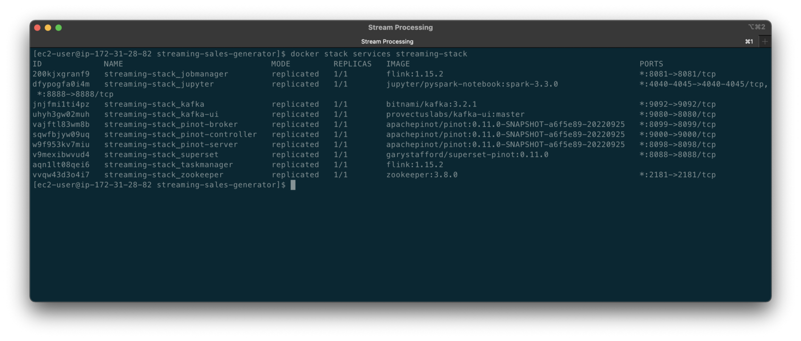
To get started, we need to replace the first streaming Docker Swarm stack, deployed in part one, with the second streaming Docker Swarm stack. The second stack contains Apache Kafka, Apache Zookeeper, Apache Flink, Apache Pinot, Apache Superset, UI for Apache Kafka, and Project Jupyter (JupyterLab).
https://programmaticponderings.wordpress.com/media/601efca17604c3a467a4200e93d7d3ff
The stack will take a few minutes to deploy fully. When complete, there should be ten containers running in the stack.
Flink Application
The Flink application has two entry classes. The first class, RunningTotals, performs an identical aggregation function as the previous KStreams demo.
The second class, JoinStreams, joins the stream of data from the demo.purchases topic and the demo.products topic, processing and combining them, in real-time, into an enriched transaction and publishing the results to a new topic, demo.purchases.enriched.
The resulting enriched purchases messages look similar to the following:
Running the Flink Job
To run the Flink application, we must first compile it into an uber JAR.
We can copy the JAR into the Flink container or upload it through the Apache Flink Dashboard, a browser-based UI. For this demonstration, we will upload it through the Apache Flink Dashboard, accessible on port 8081.
The project’s build.gradle file has preset the Main class (Flink’s Entry class) to org.example.JoinStreams. Optionally, to run the Running Totals demo, we could change the build.gradle file and recompile, or simply change Flink’s Entry class to org.example.RunningTotals.

Before running the Flink job, restart the sales generator in the background (nohup python3 ./producer.py &) to generate a new stream of data. Then start the Flink job.

To confirm the Flink application is running, we can check the contents of the new demo.purchases.enriched topic using the Kafka CLI.

Alternatively, you can use the UI for Apache Kafka, accessible on port 9080.

Demonstration #4: Apache Pinot
In the fourth and final demonstration, we will explore Apache Pinot. First, we will query the unbounded data streams from Apache Kafka, generated by both the sales generator and the Apache Flink application, using SQL. Then, we build a real-time dashboard in Apache Superset, with Apache Pinot as our datasource.

Creating Tables
According to the Apache Pinot documentation, “a table is a logical abstraction that represents a collection of related data. It is composed of columns and rows (known as documents in Pinot).” There are three types of Pinot tables: Offline, Realtime, and Hybrid. For this demonstration, we will create three Realtime tables. Realtime tables ingest data from streams — in our case, Kafka — and build segments from the consumed data. Further, according to the documentation, “each table in Pinot is associated with a Schema. A schema defines what fields are present in the table along with the data types. The schema is stored in Zookeeper, along with the table configuration.”
Below, we see the schema and config for one of the three Realtime tables, purchasesEnriched. Note how the columns are divided into three categories: Dimension, Metric, and DateTime.
To begin, copy the three Pinot Realtime table schemas and configurations from the streaming-sales-generator GitHub project into the Apache Pinot Controller container. Next, use a docker exec command to call the Pinot Command Line Interface’s (CLI) AddTable command to create the three tables: products, purchases, and purchasesEnriched.
To confirm the three tables were created correctly, use the Apache Pinot Data Explorer accessible on port 9000. Use the Tables tab in the Cluster Manager.

We can further inspect and edit the table’s config and schema from the Tables tab in the Cluster Manager.

The three tables are configured to read the unbounded stream of data from the corresponding Kafka topics: demo.products, demo.purchases, and demo.purchases.enriched.
Querying with Pinot
We can use Pinot’s Query Console to query the Realtime tables using SQL. According to the documentation, “Pinot provides a SQL interface for querying. It uses the [Apache] Calcite SQL parser to parse queries and uses MYSQL_ANSI dialect.”

With the generator still running, re-query the purchases table in the Query Console (select count(*) from purchases). You should notice the document count increasing each time you re-run the query since new messages are published to the demo.purchases topic by the sales generator.
If you do not observe the count increasing, ensure the sales generator and Flink enrichment job are running.

Table Joins?
It might seem logical to want to replicate the same multi-stream join we performed with Apache Flink in part three of the demonstration on the demo.products and demo.purchases topics. Further, we might presume to join the products and purchases realtime tables by writing a SQL statement in Pinot’s Query Console. However, according to the documentation, at the time of this post, version 0.11.0 of Pinot did not [currently] support joins or nested subqueries.
This current join limitation is why we created the Realtime table, purchasesEnriched, allowing us to query Flink’s real-time results in the demo.purchases.enriched topic. We will use both Flink and Pinot as part of our stream processing pipeline, taking advantage of each tool’s individual strengths and capabilities.
Note, according to the documentation for the latest release of Pinot on the main branch, “the latest Pinot multi-stage supports inner join, left-outer, semi-join, and nested queries out of the box. It is optimized for in-memory process and latency.” For more information on joins as part of Pinot’s new multi-stage query execution engine, read the documentation, Multi-Stage Query Engine.

demo.purchases.enriched topic in real-timeAggregations
We can perform real-time aggregations using Pinot’s rich SQL query interface. For example, like previously with Spark and Flink, we can calculate running totals for the number of items sold and the total sales for each product in real time.

We can do the same with the purchasesEnriched table, which will use the continuous stream of enriched transaction data from our Apache Flink application. With the purchasesEnriched table, we can add the product name and product category for richer results. Each time we run the query, we get real-time results based on the running sales generator and Flink enrichment job.

Query Options and Indexing
Note the reference to the Star-Tree index at the start of the SQL query shown above. Pinot provides several query options, including useStarTree (true by default).
Multiple indexing techniques are available in Pinot, including Forward Index, Inverted Index, Star-tree Index, Bloom Filter, and Range Index, among others. Each has advantages in different query scenarios. According to the documentation, by default, Pinot creates a dictionary-encoded forward index for each column.
SQL Examples
Here are a few examples of SQL queries you can try in Pinot’s Query Console:
Troubleshooting Pinot
If have issues with creating the tables or querying the real-time data, you can start by reviewing the Apache Pinot logs:
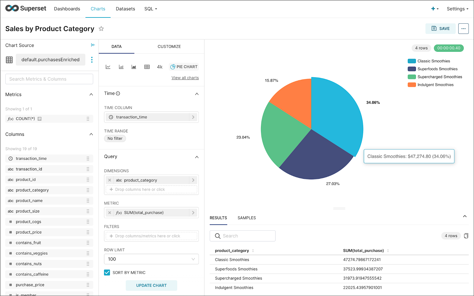
Real-time Dashboards with Apache Superset
To display the real-time stream of data produced results of our Apache Flink stream processing job and made queriable by Apache Pinot, we can use Apache Superset. Superset positions itself as “a modern data exploration and visualization platform.” Superset allows users “to explore and visualize their data, from simple line charts to highly detailed geospatial charts.”
According to the documentation, “Superset requires a Python DB-API database driver and a SQLAlchemy dialect to be installed for each datastore you want to connect to.” In the case of Apache Pinot, we can use pinotdb as the Python DB-API and SQLAlchemy dialect for Pinot. Since the existing Superset Docker container does not have pinotdb installed, I have built and published a Docker Image with the driver and deployed it as part of the second streaming stack of containers.
First, we much configure the Superset container instance. These instructions are documented as part of the Superset Docker Image repository.
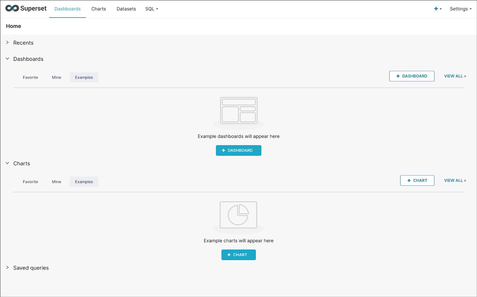
Once the configuration is complete, we can log into the Superset web-browser-based UI accessible on port 8088.
Pinot Database Connection and Dataset
Next, to connect to Pinot from Superset, we need to create a Database Connection and a Dataset.
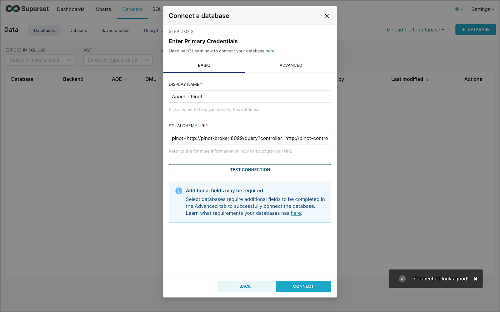
The SQLAlchemy URI is shown below. Input the URI, test your connection (‘Test Connection’), make sure it succeeds, then hit ‘Connect’.
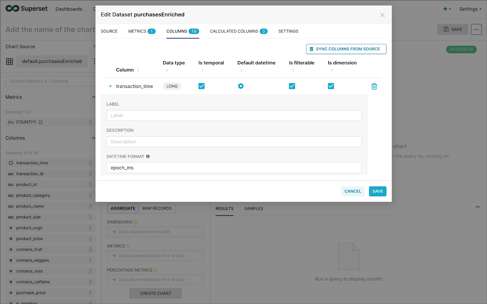
Next, create a Dataset that references the purchasesEnriched Pinot table.

purchasesEnriched Pinot tableModify the dataset’s transaction_time column. Check the is_temporal and Default datetime options. Lastly, define the DateTime format as epoch_ms.
transaction_time columnBuilding a Real-time Dashboard
Using the new dataset, which connects Superset to the purchasesEnriched Pinot table, we can construct individual charts to be placed on a dashboard. Build a few charts to include on your dashboard.
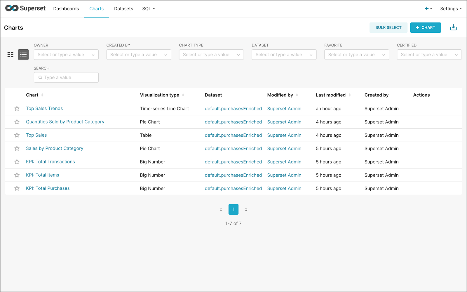
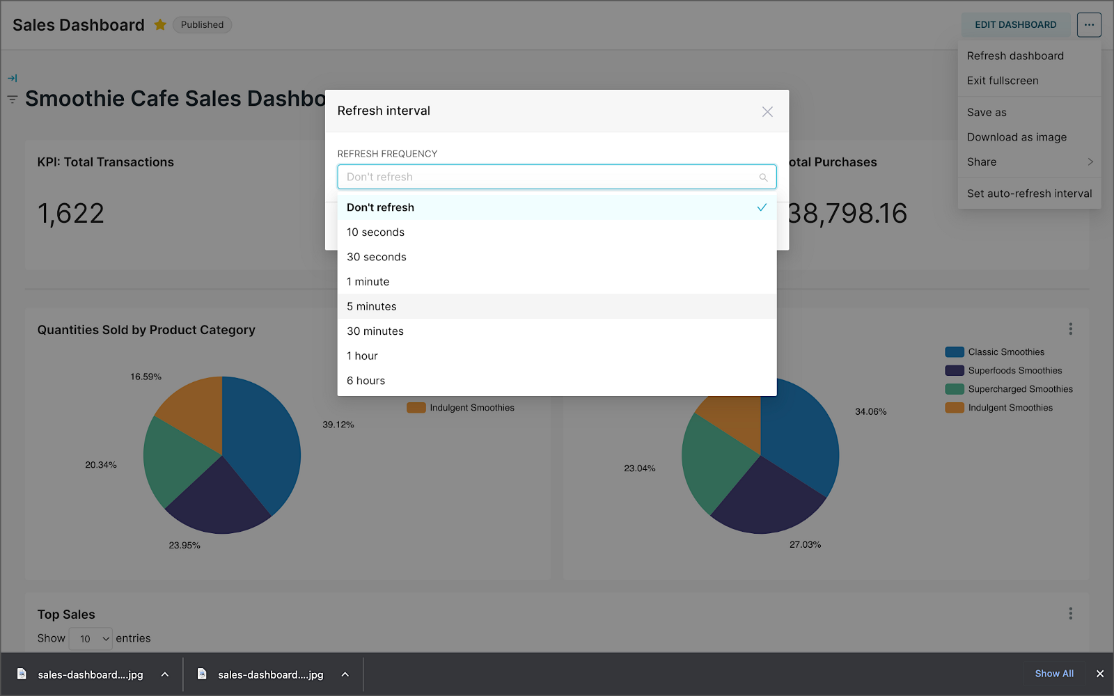
Create a new Superset dashboard and add the charts and other elements, such as headlines, dividers, and tabs.

We can apply a refresh interval to the dashboard to continuously query Pinot and visualize the results in near real-time.
Conclusion
In this two-part post series, we were introduced to stream processing. We explored four popular open-source stream processing projects: Apache Spark Structured Streaming, Apache Kafka Streams, Apache Flink, and Apache Pinot. Next, we learned how we could solve similar stream processing and streaming analytics challenges using different streaming technologies. Lastly, we saw how these technologies, such as Kafka, Flink, Pinot, and Superset, could be integrated to create effective stream processing pipelines.
This blog represents my viewpoints and not of my employer, Amazon Web Services (AWS). All product names, logos, and brands are the property of their respective owners. All diagrams and illustrations are the property of the author unless otherwise noted.
Exploring Popular Open-source Stream Processing Technologies: Part 1 of 2
Posted by Gary A. Stafford in Analytics, Big Data, Java Development, Python, Software Development, SQL on September 24, 2022
A brief demonstration of Apache Spark Structured Streaming, Apache Kafka Streams, Apache Flink, and Apache Pinot with Apache Superset
Introduction
According to TechTarget, “Stream processing is a data management technique that involves ingesting a continuous data stream to quickly analyze, filter, transform or enhance the data in real-time. Once processed, the data is passed off to an application, data store, or another stream processing engine.” Confluent, a fully-managed Apache Kafka market leader, defines stream processing as “a software paradigm that ingests, processes, and manages continuous streams of data while they’re still in motion.”
Batch vs. Stream Processing
Again, according to Confluent, “Batch processing is when the processing and analysis happens on a set of data that have already been stored over a period of time.” A batch processing example might include daily retail sales data, which is aggregated and tabulated nightly after the stores close. Conversely, “streaming data processing happens as the data flows through a system. This results in analysis and reporting of events as it happens.” To use a similar example, instead of nightly batch processing, the streams of sales data are processed, aggregated, and analyzed continuously throughout the day — sales volume, buying trends, inventory levels, and marketing program performance are tracked in real time.
Bounded vs. Unbounded Data
According to Packt Publishing’s book, Learning Apache Apex, “bounded data is finite; it has a beginning and an end. Unbounded data is an ever-growing, essentially infinite data set.” Batch processing is typically performed on bounded data, whereas stream processing is most often performed on unbounded data.
Stream Processing Technologies
There are many technologies available to perform stream processing. These include proprietary custom software, commercial off-the-shelf (COTS) software, fully-managed service offerings from Software as a Service (or SaaS) providers, Cloud Solution Providers (CSP), Commercial Open Source Software (COSS) companies, and popular open-source projects from the Apache Software Foundation and Linux Foundation.
The following two-part post and forthcoming video will explore four popular open-source software (OSS) stream processing projects, including Apache Spark Structured Streaming, Apache Kafka Streams, Apache Flink, and Apache Pinot. Each of these projects has some equivalent SaaS, CSP, and COSS offerings.
This post uses the open-source projects, making it easier to follow along with the demonstration and keeping costs to a minimum. However, you could easily substitute the open-source projects for your preferred SaaS, CSP, or COSS service offerings.
Apache Spark Structured Streaming
According to the Apache Spark documentation, “Structured Streaming is a scalable and fault-tolerant stream processing engine built on the Spark SQL engine. You can express your streaming computation the same way you would express a batch computation on static data.” Further, “Structured Streaming queries are processed using a micro-batch processing engine, which processes data streams as a series of small batch jobs thereby achieving end-to-end latencies as low as 100 milliseconds and exactly-once fault-tolerance guarantees.” In the post, we will examine both batch and stream processing using a series of Apache Spark Structured Streaming jobs written in PySpark.

Apache Kafka Streams
According to the Apache Kafka documentation, “Kafka Streams [aka KStreams] is a client library for building applications and microservices, where the input and output data are stored in Kafka clusters. It combines the simplicity of writing and deploying standard Java and Scala applications on the client side with the benefits of Kafka’s server-side cluster technology.” In the post, we will examine a KStreams application written in Java that performs stream processing and incremental aggregation.

Apache Flink
According to the Apache Flink documentation, “Apache Flink is a framework and distributed processing engine for stateful computations over unbounded and bounded data streams. Flink has been designed to run in all common cluster environments, perform computations at in-memory speed and at any scale.” Further, “Apache Flink excels at processing unbounded and bounded data sets. Precise control of time and state enables Flink’s runtime to run any kind of application on unbounded streams. Bounded streams are internally processed by algorithms and data structures that are specifically designed for fixed-sized data sets, yielding excellent performance.” In the post, we will examine a Flink application written in Java, which performs stream processing, incremental aggregation, and multi-stream joins.

Apache Pinot
According to Apache Pinot’s documentation, “Pinot is a real-time distributed OLAP datastore, purpose-built to provide ultra-low-latency analytics, even at extremely high throughput. It can ingest directly from streaming data sources — such as Apache Kafka and Amazon Kinesis — and make the events available for querying instantly. It can also ingest from batch data sources such as Hadoop HDFS, Amazon S3, Azure ADLS, and Google Cloud Storage.” In the post, we will query the unbounded data streams from Apache Kafka, generated by Apache Flink, using SQL.

Streaming Data Source
We must first find a good unbounded data source to explore or demonstrate these streaming technologies. Ideally, the streaming data source should be complex enough to allow multiple types of analyses and visualize different aspects with Business Intelligence (BI) and dashboarding tools. Additionally, the streaming data source should possess a degree of consistency and predictability while displaying a reasonable level of variability and randomness.
To this end, we will use the open-source Streaming Synthetic Sales Data Generator project, which I have developed and made available on GitHub. This project’s highly-configurable, Python-based, synthetic data generator generates an unbounded stream of product listings, sales transactions, and inventory restocking activities to a series of Apache Kafka topics.

Source Code
All the source code demonstrated in this post is open source and available on GitHub. There are three separate GitHub projects:
Docker
To make it easier to follow along with the demonstration, we will use Docker Swarm to provision the streaming tools. Alternatively, you could use Kubernetes (e.g., creating a Helm chart) or your preferred CSP or SaaS managed services. Nothing in this demonstration requires you to use a paid service.
The two Docker Swarm stacks are located in the Streaming Synthetic Sales Data Generator project:
- Streaming Stack — Part 1: Apache Kafka, Apache Zookeeper, Apache Spark, UI for Apache Kafka, and the KStreams application
- Streaming Stack — Part 2: Apache Kafka, Apache Zookeeper, Apache Flink, Apache Pinot, Apache Superset, UI for Apache Kafka, and Project Jupyter (JupyterLab).*
* the Jupyter container can be used as an alternative to the Spark container for running PySpark jobs (follow the same steps as for Spark, below)
Demonstration #1: Apache Spark
In the first of four demonstrations, we will examine two Apache Spark Structured Streaming jobs, written in PySpark, demonstrating both batch processing (spark_batch_kafka.py) and stream processing (spark_streaming_kafka.py). We will read from a single stream of data from a Kafka topic, demo.purchases, and write to the console.

Deploying the Streaming Stack
To get started, deploy the first streaming Docker Swarm stack containing the Apache Kafka, Apache Zookeeper, Apache Spark, UI for Apache Kafka, and the KStreams application containers.
The stack will take a few minutes to deploy fully. When complete, there should be a total of six containers running in the stack.

Sales Generator
Before starting the streaming data generator, confirm or modify the configuration/configuration.ini. Three configuration items, in particular, will determine how long the streaming data generator runs and how much data it produces. We will set the timing of transaction events to be generated relatively rapidly for test purposes. We will also set the number of events high enough to give us time to explore the Spark jobs. Using the below settings, the generator should run for an average of approximately 50–60 minutes: (((5 sec + 2 sec)/2)*1000 transactions)/60 sec=~58 min on average. You can run the generator again if necessary or increase the number of transactions.
Start the streaming data generator as a background service:
The streaming data generator will start writing data to three Apache Kafka topics: demo.products, demo.purchases, and demo.inventories. We can view these topics and their messages by logging into the Apache Kafka container and using the Kafka CLI:
Below, we see a few sample messages from the demo.purchases topic:

demo.purchases topicAlternatively, you can use the UI for Apache Kafka, accessible on port 9080.

demo.purchases topic in the UI for Apache Kafka
demo.purchases topic using the UI for Apache KafkaPrepare Spark
Next, prepare the Spark container to run the Spark jobs:
Running the Spark Jobs
Next, copy the jobs from the project to the Spark container, then exec back into the container:
Batch Processing with Spark
The first Spark job, spark_batch_kafka.py, aggregates the number of items sold and the total sales for each product, based on existing messages consumed from the demo.purchases topic. We use the PySpark DataFrame class’s read() and write() methods in the first example, reading from Kafka and writing to the console. We could just as easily write the results back to Kafka.
The batch processing job sorts the results and outputs the top 25 items by total sales to the console. The job should run to completion and exit successfully.

To run the batch Spark job, use the following commands:
Stream Processing with Spark
The stream processing Spark job, spark_streaming_kafka.py, also aggregates the number of items sold and the total sales for each item, based on messages consumed from the demo.purchases topic. However, as shown in the code snippet below, this job continuously aggregates the stream of data from Kafka, displaying the top ten product totals within an arbitrary ten-minute sliding window, with a five-minute overlap, and updates output every minute to the console. We use the PySpark DataFrame class’s readStream() and writeStream() methods as opposed to the batch-oriented read() and write() methods in the first example.
Shorter event-time windows are easier for demonstrations — in Production, hourly, daily, weekly, or monthly windows are more typical for sales analysis.

To run the stream processing Spark job, use the following commands:
We could just as easily calculate running totals for the stream of sales data versus aggregations over a sliding event-time window (example job included in project).

Be sure to kill the stream processing Spark jobs when you are done, or they will continue to run, awaiting more data.
Demonstration #2: Apache Kafka Streams
Next, we will examine Apache Kafka Streams (aka KStreams). For this part of the post, we will also use the second of the three GitHub repository projects, kstreams-kafka-demo. The project contains a KStreams application written in Java that performs stream processing and incremental aggregation.
KStreams Application
The KStreams application continuously consumes the stream of messages from the demo.purchases Kafka topic (source) using an instance of the StreamBuilder() class. It then aggregates the number of items sold and the total sales for each item, maintaining running totals, which are then streamed to a new demo.running.totals topic (sink). All of this using an instance of the KafkaStreams() Kafka client class.
Running the Application
We have at least three choices to run the KStreams application for this demonstration: 1) running locally from our IDE, 2) a compiled JAR run locally from the command line, or 3) a compiled JAR copied into a Docker image, which is deployed as part of the Swarm stack. You can choose any of the options.
Compiling and running the KStreams application locally
We will continue to use the same streaming Docker Swarm stack used for the Apache Spark demonstration. I have already compiled a single uber JAR file using OpenJDK 17 and Gradle from the project’s source code. I then created and published a Docker image, which is already part of the running stack.
Since we ran the sales generator earlier for the Spark demonstration, there is existing data in the demo.purchases topic. Re-run the sales generator (nohup python3 ./producer.py &) to generate a new stream of data. View the results of the KStreams application, which has been running since the stack was deployed using the Kafka CLI or UI for Apache Kafka:
Below, in the top terminal window, we see the output from the KStreams application. Using KStream’s peek() method, the application outputs Purchase and Total instances to the console as they are processed and written to Kafka. In the lower terminal window, we see new messages being published as a continuous stream to output topic, demo.running.totals.

Part Two
In part two of this two-part post, we continue our exploration of the four popular open-source stream processing projects. We will cover Apache Flink and Apache Pinot. In addition, we will incorporate Apache Superset into the demonstration, building a real-time dashboard to visualize the results of our stream processing.
This blog represents my viewpoints and not of my employer, Amazon Web Services (AWS). All product names, logos, and brands are the property of their respective owners. All diagrams and illustrations are the property of the author unless otherwise noted.
The Art of Building Open Data Lakes with Apache Hudi, Kafka, Hive, and Debezium
Posted by Gary A. Stafford in Analytics, AWS, Big Data, Cloud, Python, Software Development, Technology Consulting on December 31, 2021
Build near real-time, open-source data lakes on AWS using a combination of Apache Kafka, Hudi, Spark, Hive, and Debezium
Introduction
In the following post, we will learn how to build a data lake on AWS using a combination of open-source software (OSS), including Red Hat’s Debezium, Apache Kafka, Kafka Connect, Apache Hive, Apache Spark, Apache Hudi, and Hudi DeltaStreamer. We will use fully-managed AWS services to host the datasource, the data lake, and the open-source tools. These services include Amazon RDS, MKS, EKS, EMR, and S3.

This post is an in-depth follow-up to the video demonstration, Building Open Data Lakes on AWS with Debezium and Apache Hudi.
Workflow
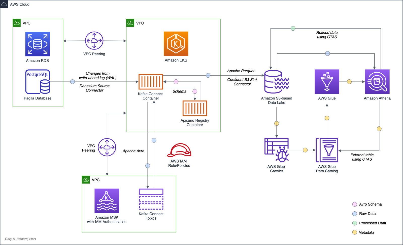
As shown in the architectural diagram above, these are the high-level steps in the demonstration’s workflow:
- Changes (inserts, updates, and deletes) are made to the datasource, a PostgreSQL database running on Amazon RDS;
- Kafka Connect Source Connector, utilizing Debezium and running on Amazon EKS (Kubernetes), continuously reads data from PostgreSQL WAL using Debezium;
- Source Connector creates and stores message schemas in Apicurio Registry, also running on Amazon EKS, in Avro format;
- Source Connector transforms and writes data in Apache Avro format to Apache Kafka, running on Amazon MSK;
- Kafka Connect Sink Connector, using Confluent S3 Sink Connector, reads messages from Kafka topics using schemas from Apicurio Registry;
- Sink Connector writes data to Amazon S3 in Apache Avro format;
- Apache Spark, using Hudi DeltaStreamer and running on Amazon EMR, reads message schemas from Apicurio Registry;
- DeltaStreamer reads raw Avro-format data from Amazon S3;
- DeltaStreamer writes data to Amazon S3 as both Copy on Write (CoW) and Merge on Read (MoR) table types;
- DeltaStreamer syncs Hudi tables and partitions to Apache Hive running on Amazon EMR;
- Queries are executed against Apache Hive Metastore or directly against Hudi tables using Apache Spark, with data returned from Hudi tables in Amazon S3;
The workflow described above actually contains two independent processes running simultaneously. Steps 2–6 represent the first process, the change data capture (CDC) process. Kafka Connect is used to continuously move changes from the database to Amazon S3. Steps 7–10 represent the second process, the data lake ingestion process. Hudi’s DeltaStreamer reads raw CDC data from Amazon S3 and writes the data back to another location in S3 (the data lake) in Apache Hudi table format. When combined, these processes can give us near real-time, incremental data ingestion of changes from the datasource to the Hudi-managed data lake.
Alternatives
This demonstration’s workflow is only one of many possible workflows to achieve similar outcomes. Alternatives include:
- Replace self-managed Kafka Connect with the fully-managed Amazon MSK Connect service.
- Exchange Amazon EMR for AWS Glue Jobs or AWS Glue Studio and the custom AWS Glue Connector for Apache Hudi to ingest data into Hudi tables.
- Replace Apache Hive with AWS Glue Data Catalog, a fully-managed Hive-compatible metastore.
- Replace Apicurio Registry with Confluent Schema Registry or AWS Glue Schema Registry.
- Exchange the Confluent S3 Sink Connector for the Kafka Connect Sink for Hudi, which could greatly simplify the workflow.
- Substitute
HoodieMultiTableDeltaStreamerfor theHoodieDeltaStreamerutility to quickly ingest multiple tables into Hudi. - Replace Hudi’s AvroDFSSource for the AvroKafkaSource to read directly from Kafka versus Amazon S3, or Hudi’s JdbcSource to read directly from the PostgreSQL database. Hudi has several datasource readers available. Be cognizant of authentication/authorization compatibility/limitations.
- Choose either or both Hudi’s Copy on Write (CoW) and Merge on Read (MoR) table types depending on your workload requirements.
Source Code
All source code for this post and the previous posts in this series are open-sourced and located on GitHub. The specific resources used in this post are found in the debezium_hudi_demo directory of the GitHub repository. There are also two copies of the Museum of Modern Art (MoMA) Collection dataset from Kaggle, specifically prepared for this post, located in the moma_data directory. One copy is a nearly full dataset, and the other is a smaller, cost-effective dev/test version.
Kafka Connect
In this demonstration, Kafka Connect runs on Kubernetes, hosted on the fully-managed Amazon Elastic Kubernetes Service (Amazon EKS). Kafka Connect runs the Source and Sink Connectors.
Source Connector
The Kafka Connect Source Connector, source_connector_moma_postgres_kafka.json, used in steps 2–4 of the workflow, utilizes Debezium to continuously read changes to an Amazon RDS for PostgreSQL database. The PostgreSQL database hosts the MoMA Collection in two tables: artists and artworks.
The Debezium Connector for PostgreSQL reads record-level insert, update, and delete entries from PostgreSQL’s write-ahead log (WAL). According to the PostgreSQL documentation, changes to data files must be written only after log records describing the changes have been flushed to permanent storage, thus the name, write-ahead log. The Source Connector then creates and stores Apache Avro message schemas in Apicurio Registry also running on Amazon EKS.


Finally, the Source Connector transforms and writes Avro format messages to Apache Kafka running on the fully-managed Amazon Managed Streaming for Apache Kafka (Amazon MSK). Assuming Kafka’s topic.creation.enable property is set to true, Kafka Connect will create any necessary Kafka topics, one per database table.
Below, we see an example of a Kafka message representing an insert of a record with the artist_id 1 in the MoMA Collection database’s artists table. The record was read from the PostgreSQL WAL, transformed, and written to a corresponding Kafka topic, using the Debezium Connector for PostgreSQL. The first version represents the raw data before being transformed by Debezium. Note that the type of operation (_op) indicates a read (r). Possible values include c for create (or insert), u for update, d for delete, and r for read (applies to snapshots).
The next version represents the same record after being transformed by Debezium using the event flattening single message transformation (unwrap SMT). The final message structure represents the schema stored in Apicurio Registry. The message structure is identical to the structure of the data written to Amazon S3 by the Sink Connector.
Sink Connector
The Kafka Connect Sink Connector, sink_connector_moma_kafka_s3.json, used in steps 5–6 of the workflow, implements the Confluent S3 Sink Connector. The Sink Connector reads the Avro-format messages from Kafka using the schemas stored in Apicurio Registry. It then writes the data to Amazon S3, also in Apache Avro format, based on the same schemas.
Running Kafka Connect
We first start Kafka Connect in the background to be the CDC process.
Then, deploy the Kafka Connect Source and Sink Connectors using Kafka Connect’s RESTful API. Using the API, we can also confirm the status of the Connectors.
To confirm the two Kafka topics, moma.public.artists and moma.public.artworks, were created and contain Avro messages, we can use Kafka’s command-line tools.
In the short video-only clip below, we see the process of deploying the Kafka Connect Source and Sink Connectors and confirming they are working as expected.
The Sink Connector writes data to Amazon S3 in batches of 10k messages or every 60 seconds (one-minute intervals). These settings are configurable and highly dependent on your requirements, including message volume, message velocity, real-time analytics requirements, and available compute resources.

Since we will not be querying this raw Avro-format CDC data in Amazon S3 directly, there is no need to catalog this data in Apache Hive or AWS Glue Data Catalog, a fully-managed Hive-compatible metastore.
Apache Hudi
According to the overview, Apache Hudi (pronounced “hoodie”) is the next-generation streaming data lake platform. Apache Hudi brings core warehouse and database functionality to data lakes. Hudi provides tables, transactions, efficient upserts and deletes, advanced indexes, streaming ingestion services, data clustering, compaction optimizations, and concurrency, all while keeping data in open source file formats.
Without Hudi or an equivalent open-source data lake table format such as Apache Iceberg or Databrick’s Delta Lake, most data lakes are just of bunch of unmanaged flat files. Amazon S3 cannot natively maintain the latest view of the data, to the surprise of many who are more familiar with OLTP-style databases or OLAP-style data warehouses.
DeltaStreamer
DeltaStreamer, aka the HoodieDeltaStreamer utility (part of the hudi-utilities-bundle), used in steps 7–10 of the workflow, provides the way to perform streaming ingestion of data from different sources such as Distributed File System (DFS) and Apache Kafka.
Optionally, HoodieMultiTableDeltaStreamer, a wrapper on top of HoodieDeltaStreamer, ingests multiple tables in a single Spark job, into Hudi datasets. Currently, it only supports sequential processing of tables to be ingested and Copy on Write table type.
We are using HoodieDeltaStreamer to write to both Merge on Read (MoR) and Copy on Write (CoW) table types for demonstration purposes only. The MoR table type is a superset of the CoW table type, which stores data using a combination of columnar-based (e.g., Apache Parquet) plus row-based (e.g., Apache Avro) file formats. Updates are logged to delta files and later compacted to produce new versions of columnar files synchronously or asynchronously. Again, the choice of table types depends on your requirements.

Amazon EMR
For this demonstration, I’ve used the recently released Amazon EMR version 6.5.0 configured with Apache Spark 3.1.2 and Apache Hive 3.1.2. EMR 6.5.0 runs Scala version 2.12.10, Python 3.7.10, and OpenJDK Corretto-8.312. I have included the AWS CloudFormation template and parameters file used to create the EMR cluster, on GitHub.

When choosing Apache Spark, Apache Hive, or Presto on EMR 6.5.0, Apache Hudi release 0.9.0 is automatically installed.

DeltaStreamer Configuration
Below, we see the DeltaStreamer properties file, deltastreamer_artists_apicurio_mor.properties. This properties file is referenced by the Spark job that runs DeltaStreamer, shown next. The file contains properties related to the datasource, the data sink, and Apache Hive. The source of the data for DeltaStreamer is the CDC data written to Amazon S3. In this case, the datasource is the objects located in the /topics/moma.public.artworks/partition=0/ S3 object prefix. The data sink is a Hudi MoR table type in Amazon S3. DeltaStreamer will write Parquet data, partitioned by the artist’s nationality, to the /moma_mor/artists/ S3 object prefix. Lastly, DeltaStreamer will sync all tables and table partitions to Apache Hive, including creating the Hive databases and tables if they do not already exist.
Below, we see the equivalent DeltaStreamer properties file for the MoMA artworks, deltastreamer_artworks_apicurio_mor.properties. There are also comparable DeltaStreamer property files for the Hudi CoW tables on GitHub.
All DeltaStreamer property files reference Apicurio Registry for the location of the Avro schemas. The schemas are used by both the Kafka Avro-format messages and the CDC-created Avro-format files in Amazon S3. Due to DeltaStreamer’s coupling with Confluent Schema Registry, as opposed to other registries, we must use Apicurio Registry’s Confluent Schema Registry API (Version 6) compatibility API endpoints (e.g., /apis/ccompat/v6/subjects/moma.public.artists-value/versions/latest) when using the org.apache.hudi.utilities.schema.SchemaRegistryProvider datasource option with DeltaStreamer. According to Apicurio, to provide compatibility with Confluent SerDes (Serializer/Deserializer) and other clients, Apicurio Registry implements the API defined by the Confluent Schema Registry.

Running DeltaStreamer
The properties files are loaded by Spark jobs that call the DeltaStreamer library, using spark-submit. Below, we see an example Spark job that calls the DeltaStreamer class. DeltaStreamer reads the raw Avro-format CDC data from S3 and writes the data using the Hudi MoR table type into the /moma_mor/artists/ S3 object prefix. In this Spark particular job, we are using the continuous option. DeltaStreamer runs in continuous mode using this option, running source-fetch, transform, and write in a loop. We are also using the UPSERT write operation (op). Operation options include UPSERT, INSERT, and BULK_INSERT. This set of options is ideal for inserting ongoing changes to CDC data into Hudi tables. You can run jobs in the foreground or background on EMR’s Master Node or as EMR Steps from the Amazon EMR console.
Below, we see another example DeltaStreamer Spark job that reads the raw Avro-format CDC data from S3 and writes the data using the MoR table type into the /moma_mor/artworks/ S3 object prefix. This example uses the BULK_INSERT write operation (op) and the filter-dupes option. The filter-dupes option ensures that should duplicate records from the source are dropped/filtered out before INSERT or BULK_INSERT. This set of options is ideal for the initial bulk inserting of existing data into Hudi tables. The job runs one time and completes, unlike the previous example that ran continuously.
Syncing with Hive
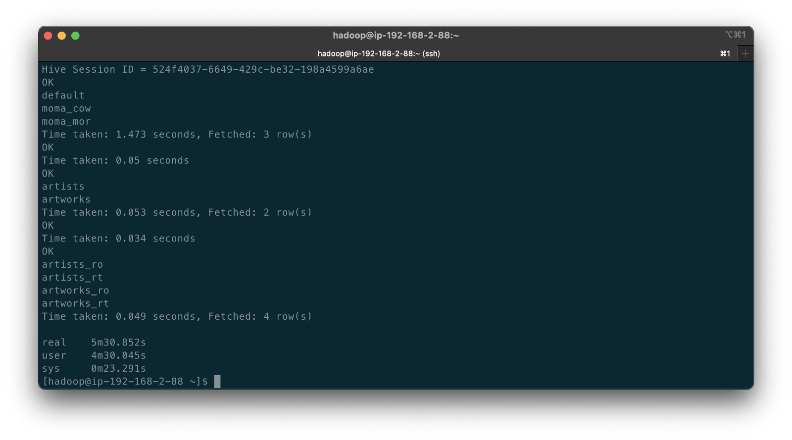
The following abridged, video-only clip demonstrates the differences between the Hudi CoW and MoR table types with respect to Apache Hive. In the video, we run the deltastreamer_jobs_bulk_bkgd.sh script, included on GitHub. This script runs four different Apache Spark jobs, using Hudi DeltaStreamer to bulk-ingest all the artists and artworks CDC data from Amazon S3 into both Hudi CoW and MoR table types. Once the four Spark jobs are complete, the script queries Apache Hive and displays the new Hive databases and database tables created by DeltaStreamer.
In both the video above and terminal screengrab below, note the difference in the tables created within the two Hive databases, the Hudi CoW table type (moma_cow) and the MoR table type (moma_mor). The MoR table type creates both a read-optimized table (_ro) as well as a real-time table (_rt) for each datasource (e.g., artists_ro and artists_rt).
According to documentation, Hudi creates two tables in the Hive metastore for the MoR table type. The first, a table which is a read-optimized view appended with _ro and the second, a table with the same name appended with _rt which is a real-time view. According to Hudi, the read-optimized view exposes columnar Parquet while the real-time view exposes columnar Parquet and/or row-based logs; you can query both tables. The CoW table type creates a single table without a suffix for each datasource (e.g., artists). Below, we see the Hive table structure for the artists_rt table, created by DeltaStreamer, using SHOW CREATE TABLE moma_mor.artists_rt;.
Having run the demonstration’s deltastreamer_jobs_bulk_bkgd.sh script, the resulting object structure in the Hudi-managed section of the Amazon S3 bucket looks as follows.

Below is an example of Hudi files created in the /moma/artists_cow/ S3 object prefix. When using data lake table formats like Hudi, given its specialized directory structure and the high number of objects, interactions with the data should be abstracted through Hudi’s programming interfaces. Generally speaking, you do not interact directly with the objects in a data lake.
Hudi CLI
Optionally, we can inspect the Hudi tables using the Hudi CLI (hudi-cli). The CLI offers an extensive list of available commands. Using the CLI, we can inspect the Hudi tables and their schemas, and review operational statistics like write amplification (the number of bytes written for 1 byte of incoming data), commits, and compactions.
The following short video-only clip shows the use of the Hudi CLI, running on the Amazon EMR Master Node, to inspect the Hudi tables in S3.
Hudi Data Structure
Recall the sample Kafka message we saw earlier in the post representing an insert of an artist record with the artist_id 1. Below, we see what the same record looks like after being ingested by Hudi DeltaStreamer. Note the five additional fields added by Hudi with the _hoodie_ prefix.
Querying Hudi-managed Data
With the initial data ingestion complete and the CDC and DeltaStreamer processes monitoring for future changes, we can query the resulting data stored in Hudi tables. First, we will make some changes to the PostgreSQL MoMA Collection database to see how Hudi manages the data mutations. We could also make changes directly to the Hudi tables using Hive, Spark, or Presto. However, that would cause our datasource to be out of sync with the Hudi tables, potentially negating the entire CDC process. When developing a data lake, this is a critically important consideration — how changes are introduced to Hudi tables, especially when CDC is involved, and whether data continuity between datasources and the data lake is essential.
For the demonstration, I have made a series of arbitrary updates to a piece of artwork in the MoMA Collection database, ‘Picador (La Pique)’ by Pablo Picasso.
Below, note the last four objects shown in S3. Judging by the file names and dates, we can see that the CDC process, using Kafka Connect, has picked up the four updates I made to the record in the database. The Source Connector first wrote the changes to Kafka. The Sink Connector then read those Kafka messages and wrote the data to Amazon S3 in Avro format, as shown below.

Looking again at S3, we can also observe that DeltaStreamer picked up the new CDC objects in Amazon S3 and wrote them to both the Hudi CoW and MoR tables. Note the file types shown below. Given Hudi’s MoR table type structure, Hudi first logged the changes to row-based delta files and later compacted them to produce a new version of the columnar-format Parquet file.

Querying Results from Apache Hive
There are several ways to query Hudi-managed data in S3. In this demonstration, they include against Apache Hive using the hive client from the command line, against Hive using Spark, and against the Hudi tables also using Spark. We could also install Presto on EMR to query the Hudi data directly or via Hive.
Querying the real-time artwork_rt table in Hive after we make each database change, we can observe the data in Hudi reflects the updates. Note that the value of the _hoodie_file_name field for the first three updates is a Hudi delta log file, while the value for the last update is a Parquet file. The Parquet file signifies compaction occurred between the fourth update was made, and the time the Hive query was executed. Lastly, note the type of operation (_op) indicates an update change (u) for all records.

Once all fours database updates are complete and compaction has occurred, we should observe identical results from all Hive tables. Below, note the _hoodie_file_name field for all three tables is a Parquet file. Logically, the Parquet file for the MoR read-optimized and real-time Hive tables is the same.

Had we queried the data previous to compaction, the results would have differed. Below we have three queries. I further updated the artwork record, changing the date field from 1959 to 1960. The read-optimized MoR table, artworks_ro, still reflects the original date value, 1959, before the update and prior to compaction. The real-time table,artworks_rt , reflects the latest update to the date field, 1960. Note that the value of the _hoodie_file_name field for the read-optimized table is a Parquet file, while the value for the real-time table (artworks_rt), the third and final query, is a delta log file. The delta log allows the real-time table to display the most current state of the data in Hudi.

Below are a few useful Hive commands to query the changes in Hudi.
Deletes with Hudi
In addition to inserts and updates (upserts), Apache Hudi can manage deletes. Hudi supports implementing two types of deletes on data stored in Hudi tables: soft deletes and hard deletes. Given this demonstration’s specific configuration for CDC and DeltaStreamer, we will use soft deletes. Soft deletes retain the record key and nullify the other field’s values. Hard deletes, a stronger form of deletion, physically remove any record trace from the Hudi table.
Below, we see the CDC record for the artist with artist_id 441. The event flattening single message transformation (SMT), used by the Debezium-based Kafka Connect Source Connector, adds the __deleted field with a value of true and nullifies all fields except the record’s key, artist_id, which is required.
Below, we see the same delete record for the artist with artist_id 441 in the Hudi MoR table. All the null fields have been removed.
Below, we see how the deleted record appears in the three Hive CoW and MoR artwork tables. Note the query results from the read-optimized MoR table, artworks_ro, contains two records — the original record (r) and the deleted record (d). The data is partitioned by nationality, and since the record was deleted, the nationality field is changed to null. In S3, Hudi represents this partition as nationality=default. The record now exists in two different Parquet files, within two separate partitions, something to be aware of when querying the read-optimized MoR table.

Time Travel
According to the documentation, Hudi has supported time travel queries since version 0.9.0. With time travel, you can query the previous state of your data. Time travel is particularly useful for use cases, including rollbacks, debugging, and audit history.
To demonstrate time travel queries in Hudi, we start by making some additional changes to the source database. For this demonstration, I made a series of five updates and finally a delete to the artist record with artist_id 299 in the PostgreSQL database over a few-hour period.
Once the CDC and DeltaStreamer ingestion processes are complete, we can use Hudi’s time travel query capability to view the state of data in Hudi at different points in time (instants). To do so, we need to provide an as.an.instant date/time value to Spark (see line 21 below).
Based on the time period in which I made the five updates and the delete, I have chosen six instants during that period where I want to examine the state of the record. Below is an example of the PySpark code from a Jupyter Notebook used to perform the six time travel queries against the Hudi MoR artist’s table.
Below, we see the results of the time travel queries. At each instant, we can observe the mutating state of the data in the Hudi MoR Artist’s table, including the initial bulk insert of the existing snapshot of data (r) and the delete record (d). Since the delete made in the PostgreSQL database was recorded as a soft delete in Hudi, as opposed to a hard delete, we are still able to retrieve the record at any instant.
In addition to time travel queries, Hudi also offers incremental queries and point in time queries.
Conclusion
Although this post only scratches the surface of the capabilities of Debezium and Hudi, you can see the power of CDC using Kafka Connect and Debezium, combined with Hudi, to build and manage open data lakes on AWS.
This blog represents my own viewpoints and not of my employer, Amazon Web Services (AWS). All product names, logos, and brands are the property of their respective owners.
Video Demonstration: Building Open Data Lakes on AWS with Debezium and Apache Hudi
Posted by Gary A. Stafford in Software Development on October 31, 2021
Build an open-source data lake on AWS using a combination of Debezium, Apache Kafka, Apache Hudi, Apache Spark, and Apache Hive
Introduction
In the following recorded demonstration, we will build a simple open data lake on AWS using a combination of open-source software (OSS), including Red Hat’s Debezium, Apache Kafka, and Kafka Connect for change data capture (CDC), and Apache Hive, Apache Spark, Apache Hudi, and Hudi’s DeltaStreamer for managing our data lake. We will use fully-managed AWS services to host the open data lake components, including Amazon RDS, Amazon MKS, Amazon EKS, and EMR.

Demonstration
Source Code
All source code for this post and the previous posts in this series are open-sourced and located on GitHub. The following files are used in the demonstration:
- MoMA data: Uncompress files and import pipe-delimited data to PostgreSQL;
base.properties: Base Hudi DeltaStreamer properties;deltastreamer_artists_file_based_schema.properties: Demo-specific Hudi DeltaStreamer properties for MoMA Artists;deltastreamer_artworks_file_based_schema.properties: Demo-specific Hudi DeltaStreamer properties for MoMA Artworks;source_connector_moma_postgres_kafka.json: Kafka Connect Source Connector (PostgreSQL to Kafka);sink_connector_moma_kafka_s3.json: Kafka Connect Sink Connector (Kafka to Amazon S3);moma_debezium_hudi_demo.ipynb: Jupyter PySpark Notebook;demonstration_notes.md: Commands used in the demonstration;
This blog represents my own viewpoints and not of my employer, Amazon Web Services (AWS). All product names, logos, and brands are the property of their respective owners.
Stream Processing with Apache Spark, Kafka, Avro, and Apicurio Registry on Amazon EMR and Amazon MSK
Posted by Gary A. Stafford in Analytics, AWS, Big Data, Cloud, Python, Software Development on September 30, 2021
Using a registry to decouple schemas from messages in an event streaming analytics architecture
Introduction
In the last post, Getting Started with Spark Structured Streaming and Kafka on AWS using Amazon MSK and Amazon EMR, we learned about Apache Spark and Spark Structured Streaming on Amazon EMR (fka Amazon Elastic MapReduce) with Amazon Managed Streaming for Apache Kafka (Amazon MSK). We consumed messages from and published messages to Kafka using both batch and streaming queries. In that post, we serialized and deserialized messages to and from JSON using schemas we defined as a StructType (pyspark.sql.types.StructType) in each PySpark script. Likewise, we constructed similar structs for CSV-format data files we read from and wrote to Amazon S3.
schema = StructType([
    StructField("payment_id", IntegerType(), False),
    StructField("customer_id", IntegerType(), False),
    StructField("amount", FloatType(), False),
    StructField("payment_date", TimestampType(), False),
    StructField("city", StringType(), True),
    StructField("district", StringType(), True),
    StructField("country", StringType(), False),
])
In this follow-up post, we will read and write messages to and from Amazon MSK in Apache Avro format. We will store the Avro-format Kafka message’s key and value schemas in Apicurio Registry and retrieve the schemas instead of hard-coding the schemas in the PySpark scripts. We will also use the registry to store schemas for CSV-format data files.
Video Demonstration
In addition to this post, there is now a video demonstration available on YouTube.
Technologies
In the last post, Getting Started with Spark Structured Streaming and Kafka on AWS using Amazon MSK and Amazon EMR, we learned about Apache Spark, Apache Kafka, Amazon EMR, and Amazon MSK.
In a previous post, Hydrating a Data Lake using Log-based Change Data Capture (CDC) with Debezium, Apicurio, and Kafka Connect on AWS, we explored Apache Avro and Apicurio Registry.
Apache Spark
Apache Spark, according to the documentation, is a unified analytics engine for large-scale data processing. Spark provides high-level APIs in Java, Scala, Python (PySpark), and R. Spark provides an optimized engine that supports general execution graphs (aka directed acyclic graphs or DAGs). In addition, Spark supports a rich set of higher-level tools, including Spark SQL for SQL and structured data processing, MLlib for machine learning, GraphX for graph processing, and Structured Streaming for incremental computation and stream processing.

Spark Structured Streaming
Spark Structured Streaming, according to the documentation, is a scalable and fault-tolerant stream processing engine built on the Spark SQL engine. You can express your streaming computation the same way you would express a batch computation on static data. The Spark SQL engine will run it incrementally and continuously and update the final result as streaming data continues to arrive. In short, Structured Streaming provides fast, scalable, fault-tolerant, end-to-end, exactly-once stream processing without the user having to reason about streaming.
Apache Avro
Apache Avro describes itself as a data serialization system. Apache Avro is a compact, fast, binary data format similar to Apache Parquet, Apache Thrift, MongoDB’s BSON, and Google’s Protocol Buffers (protobuf). However, Apache Avro is a row-based storage format compared to columnar storage formats like Apache Parquet and Apache ORC.

Avro relies on schemas. When Avro data is read, the schema used when writing it is always present. According to the documentation, schemas permit each datum to be written with no per-value overheads, making serialization fast and small. Schemas also facilitate use with dynamic scripting languages since data, together with its schema, is fully self-describing.

Apicurio Registry
We can decouple the data from its schema by using schema registries such as Confluent Schema Registry or Apicurio Registry. According to Apicurio, in a messaging and event streaming architecture, data published to topics and queues must often be serialized or validated using a schema (e.g., Apache Avro, JSON Schema, or Google Protocol Buffers). Of course, schemas can be packaged in each application. Still, it is often a better architectural pattern to register schemas in an external system [schema registry] and then reference them from each application.
It is often a better architectural pattern to register schemas in an external system and then reference them from each application.
Amazon EMR
According to AWS documentation, Amazon EMR (fka Amazon Elastic MapReduce) is a cloud-based big data platform for processing vast amounts of data using open source tools such as Apache Spark, Hadoop, Hive, HBase, Flink, Hudi, and Presto. Amazon EMR is a fully managed AWS service that makes it easy to set up, operate, and scale your big data environments by automating time-consuming tasks like provisioning capacity and tuning clusters.
Amazon EMR on EKS, a deployment option for Amazon EMR since December 2020, allows you to run Amazon EMR on Amazon Elastic Kubernetes Service (Amazon EKS). With the EKS deployment option, you can focus on running analytics workloads while Amazon EMR on EKS builds, configures, and manages containers for open-source applications.
If you are new to Amazon EMR for Spark, specifically PySpark, I recommend a recent two-part series of posts, Running PySpark Applications on Amazon EMR: Methods for Interacting with PySpark on Amazon Elastic MapReduce.
Apache Kafka
According to the documentation, Apache Kafka is an open-source distributed event streaming platform used by thousands of companies for high-performance data pipelines, streaming analytics, data integration, and mission-critical applications.
Amazon MSK
Apache Kafka clusters are challenging to set up, scale, and manage in production. According to AWS documentation, Amazon MSK is a fully managed AWS service that makes it easy for you to build and run applications that use Apache Kafka to process streaming data. With Amazon MSK, you can use native Apache Kafka APIs to populate data lakes, stream changes to and from databases, and power machine learning and analytics applications.
Prerequisites
Similar to the previous post, this post will focus primarily on configuring and running Apache Spark jobs on Amazon EMR. To follow along, you will need the following resources deployed and configured on AWS:
- Amazon S3 bucket (holds all Spark/EMR resources);
- Amazon MSK cluster (using IAM Access Control);
- Amazon EKS container or an EC2 instance with the Kafka APIs installed and capable of connecting to Amazon MSK;
- Amazon EKS container or an EC2 instance with Apicurio Registry installed and capable of connecting to Amazon MSK (if using Kafka for backend storage) and being accessed by Amazon EMR;
- Ensure the Amazon MSK Configuration has
auto.create.topics.enable=true; this setting isfalseby default;
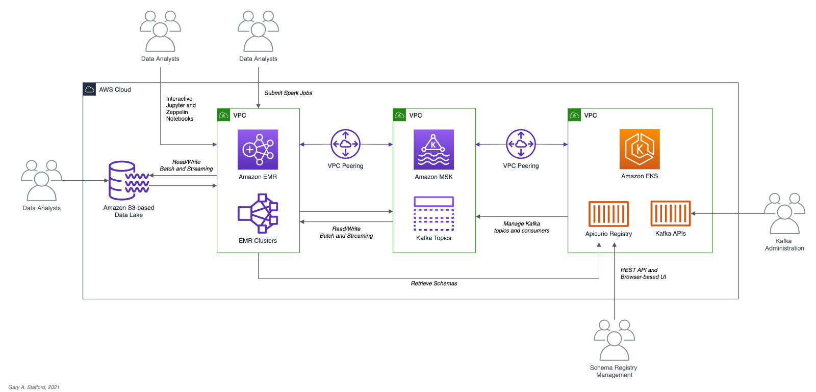
The architectural diagram below shows that the demonstration uses three separate VPCs within the same AWS account and AWS Region us-east-1, for Amazon EMR, Amazon MSK, and Amazon EKS. The three VPCs are connected using VPC Peering. Ensure you expose the correct ingress ports and the corresponding CIDR ranges within your Amazon EMR, Amazon MSK, and Amazon EKS Security Groups. For additional security and cost savings, use a VPC endpoint for private communications between Amazon EMR and Amazon S3.
Source Code
All source code for this post and the three previous posts in the Amazon MSK series, including the Python and PySpark scripts demonstrated herein, are open-sourced and located on GitHub.
Objective
We will run a Spark Structured Streaming PySpark job to consume a simulated event stream of real-time sales data from Apache Kafka. Next, we will enrich (join) that sales data with the sales region and aggregate the sales and order volumes by region within a sliding event-time window. Next, we will continuously stream those aggregated results back to Kafka. Finally, a batch query will consume the aggregated results from Kafka and display the sales results in the console.

Kafka messages will be written in Apache Avro format. The schemas for the Kafka message keys and values and the schemas for the CSV-format sales and sales regions data will all be stored in Apricurio Registry. The Python and PySpark scripts will use Apricurio Registry’s REST API to read, write, and manage the Avro schema artifacts.
We are writing the Kafka message keys in Avro format and storing an Avro key schema in the registry. This is only done for demonstration purposes and not a requirement. Kafka message keys are not required, nor is it necessary to store both the key and the value in a common format of Avro in Kafka.
Schema evolution, compatibility, and validation are important considerations, but out of scope for this post.
PySpark Scripts
PySpark, according to the documentation, is an interface for Apache Spark in Python. PySpark allows you to write Spark applications using the Python API. PySpark supports most of Spark’s features such as Spark SQL, DataFrame, Streaming, MLlib (Machine Learning), and Spark Core. There are three PySpark scripts and one new helper Python script covered in this post:
- 10_create_schemas.py: Python script creates all Avro schemas in Apricurio Registry using the REST API;
- 11_incremental_sales_avro.py: PySpark script simulates an event stream of sales data being published to Kafka over 15–20 minutes;
- 12_streaming_enrichment_avro.py: PySpark script uses a streaming query to read messages from Kafka in real-time, enriches sales data, aggregates regional sales results, and writes results back to Kafka as a stream;
- 13_batch_read_results_avro.py: PySpark script uses a batch query to read aggregated regional sales results from Kafka and display them in the console;
Preparation
To prepare your Amazon EMR resources, review the instructions in the previous post, Getting Started with Spark Structured Streaming and Kafka on AWS using Amazon MSK and Amazon EMR. Here is a recap, with a few additions required for this post.
Amazon S3
We will start by gathering and copying the necessary files to your Amazon S3 bucket. The bucket will serve as the location for the Amazon EMR bootstrap script, additional JAR files required by Spark, PySpark scripts, and CSV-format data files.
There are a set of additional JAR files required by the Spark jobs we will be running. Download the JARs from Maven Central and GitHub, and place them in the emr_jars project directory. The JARs will include AWS MSK IAM Auth, AWS SDK, Kafka Client, Spark SQL for Kafka, Spark Streaming, and other dependencies. Compared to the last post, there is one additional JAR for Avro.
Update the SPARK_BUCKET environment variable, then upload the JARs, PySpark scripts, sample data, and EMR bootstrap script from your local copy of the GitHub project repository to your Amazon S3 bucket using the AWS s3 API.
Amazon EMR
The GitHub project repository includes a sample AWS CloudFormation template and an associated JSON-format CloudFormation parameters file. The CloudFormation template, stack.yml, accepts several environment parameters. To match your environment, you will need to update the parameter values such as SSK key, Subnet, and S3 bucket. The template will build a minimally-sized Amazon EMR cluster with one master and two core nodes in an existing VPC. You can easily modify the template and parameters to meet your requirements and budget.
aws cloudformation deploy \
    --stack-name spark-kafka-demo-dev \
    --template-file ./cloudformation/stack.yml \
    --parameter-overrides file://cloudformation/dev.json \
    --capabilities CAPABILITY_NAMED_IAM
The CloudFormation template has two essential Spark configuration items — the list of applications to install on EMR and the bootstrap script deployment.
Below, we see the EMR bootstrap shell script, bootstrap_actions.sh.
The bootstrap script performed several tasks, including deploying the additional JAR files we copied to Amazon S3 earlier to EMR cluster nodes.

Parameter Store
The PySpark scripts in this demonstration will obtain configuration values from the AWS Systems Manager (AWS SSM) Parameter Store. Configuration values include a list of Amazon MSK bootstrap brokers, the Amazon S3 bucket that contains the EMR/Spark assets, and the Apicurio Registry REST API base URL. Using the Parameter Store ensures that no sensitive or environment-specific configuration is hard-coded into the PySpark scripts. Modify and execute the ssm_params.sh script to create the AWS SSM Parameter Store parameters.
Create Schemas in Apricurio Registry
To create the schemas necessary for this demonstration, a Python script is included in the project, 10_create_schemas.py. The script uses Apricurio Registry’s REST API to create six new Avro-based schema artifacts.
Apricurio Registry supports several common artifact types, including AsyncAPI specification, Apache Avro schema, GraphQL schema, JSON Schema, Apache Kafka Connect schema, OpenAPI specification, Google protocol buffers schema, Web Services Definition Language, and XML Schema Definition. We will use the registry to store Avro schemas for use with Kafka and CSV data sources and sinks.
Although Apricurio Registry does not support CSV Schema, we can store the schemas for the CSV-format sales and sales region data in the registry as JSON-format Avro schemas.
{
  "name": "Sales",
  "type": "record",
  "doc": "Schema for CSV-format sales data",
  "fields": [
    {
      "name": "payment_id",
      "type": "int"
    },
    {
      "name": "customer_id",
      "type": "int"
    },
    {
      "name": "amount",
      "type": "float"
    },
    {
      "name": "payment_date",
      "type": "string"
    },
    {
      "name": "city",
      "type": [
        "string",
        "null"
      ]
    },
    {
      "name": "district",
      "type": [
        "string",
        "null"
      ]
    },
    {
      "name": "country",
      "type": "string"
    }
  ]
}
We can then retrieve the JSON-format Avro schema from the registry, convert it to PySpark StructType, and associate it to the DataFrame used to persist the sales data from the CSV files.
root
 |-- payment_id: integer (nullable = true)
 |-- customer_id: integer (nullable = true)
 |-- amount: float (nullable = true)
 |-- payment_date: string (nullable = true)
 |-- city: string (nullable = true)
 |-- district: string (nullable = true)
 |-- country: string (nullable = true)
Using the registry allows us to avoid hard-coding the schema as a StructType in the PySpark scripts in advance.
Add the PySpark script as an EMR Step. EMR will run the Python script the same way it runs PySpark jobs.
The Python script creates six schema artifacts in Apricurio Registry, shown below in Apricurio Registry’s browser-based user interface. Schemas include two key/value pairs for two Kafka topics and two for CSV-format sales and sales region data.

You have the option of enabling validation and compatibility rules for each schema with Apricurio Registry.

Each Avro schema artifact is stored as a JSON object in the registry.

Simulate Sales Event Stream
Next, we will simulate an event stream of sales data published to Kafka over 15–20 minutes. The PySpark script, 11_incremental_sales_avro.py, reads 1,800 sales records into a DataFrame (pyspark.sql.DataFrame) from a CSV file located in S3. The script then takes each Row (pyspark.sql.Row) of the DataFrame, one row at a time, and writes them to the Kafka topic, pagila.sales.avro, adding a slight delay between each write.
The PySpark scripts first retrieve the JSON-format Avro schema for the CSV data from Apricurio Registry using the Python requests module and Apricurio Registry’s REST API (get_schema()).
{
  "name": "Sales",
  "type": "record",
  "doc": "Schema for CSV-format sales data",
  "fields": [
    {
      "name": "payment_id",
      "type": "int"
    },
    {
      "name": "customer_id",
      "type": "int"
    },
    {
      "name": "amount",
      "type": "float"
    },
    {
      "name": "payment_date",
      "type": "string"
    },
    {
      "name": "city",
      "type": [
        "string",
        "null"
      ]
    },
    {
      "name": "district",
      "type": [
        "string",
        "null"
      ]
    },
    {
      "name": "country",
      "type": "string"
    }
  ]
}
The script then creates a StructType from the JSON-format Avro schema using an empty DataFrame (struct_from_json()). Avro column types are converted to Spark SQL types. The only apparent issue is how Spark mishandles the nullable value for each column. Recognize, column nullability in Spark is an optimization statement, not an enforcement of the object type.
root
 |-- payment_id: integer (nullable = true)
 |-- customer_id: integer (nullable = true)
 |-- amount: float (nullable = true)
 |-- payment_date: string (nullable = true)
 |-- city: string (nullable = true)
 |-- district: string (nullable = true)
 |-- country: string (nullable = true)
The resulting StructType is used to read the CSV data into a DataFrame (read_from_csv()).
For Avro-format Kafka key and value schemas, we use the same method, get_schema(). The resulting JSON-format schemas are then passed to the to_avro() and from_avro() methods to read and write Avro-format messages to Kafka. Both methods are part of the pyspark.sql.avro.functions module. Avro column types are converted to and from Spark SQL types.
We must run this PySpark script, 11_incremental_sales_avro.py, concurrently with the PySpark script, 12_streaming_enrichment_avro.py, to simulate an event stream. We will start both scripts in the next part of the post.
Stream Processing with Structured Streaming
The PySpark script, 12_streaming_enrichment_avro.py, uses a streaming query to read sales data messages from the Kafka topic, pagila.sales.avro, in real-time, enriches the sales data, aggregates regional sales results, and writes the results back to Kafka in micro-batches every two minutes.
The PySpark script performs a stream-to-batch join between the streaming sales data from the Kafka topic, pagila.sales.avro, and a CSV file that contains sales regions based on the common country column. Schemas for the CSV data and the Kafka message keys and values are retrieved from Apicurio Registry using the REST API identically to the previous PySpark script.
The PySpark script then performs a streaming aggregation of the sale amount and order quantity over a sliding 10-minute event-time window, writing results to the Kafka topic, pagila.sales.summary.avro, every two minutes. Below is a sample of the resulting streaming DataFrame, written to external storage, Kafka in this case, using a DataStreamWriter interface (pyspark.sql.streaming.DataStreamWriter).
Once again, schemas for the second Kafka topic’s message key and value are retrieved from Apicurio Registry using its REST API. The key schema:
{
  "name": "Key",
  "type": "int",
  "doc": "Schema for pagila.sales.summary.avro Kafka topic key"
}
And, the value schema:
{
  "name": "Value",
  "type": "record",
  "doc": "Schema for pagila.sales.summary.avro Kafka topic value",
  "fields": [
    {
      "name": "region",
      "type": "string"
    },
    {
      "name": "sales",
      "type": "float"
    },
    {
      "name": "orders",
      "type": "int"
    },
    {
      "name": "window_start",
      "type": "long",
      "logicalType": "timestamp-millis"
    },
    {
      "name": "window_end",
      "type": "long",
      "logicalType": "timestamp-millis"
    }
  ]
}
The schema as applied to the streaming DataFrame utilizing the to_avro() method.
root
 |-- region: string (nullable = false)
 |-- sales: float (nullable = true)
 |-- orders: integer (nullable = false)
 |-- window_start: long (nullable = true)
 |-- window_end: long (nullable = true)
Submit this streaming PySpark script, 12_streaming_enrichment_avro.py, as an EMR Step.
Wait about two minutes to give this third PySpark script time to start its streaming query fully.

Then, submit the second PySpark script, 11_incremental_sales_avro.py, as an EMR Step. Both PySpark scripts will run concurrently on your Amazon EMR cluster or using two different clusters.
The PySpark script, 11_incremental_sales_avro.py, should run for approximately 15–20 minutes.

During that time, every two minutes, the script, 12_streaming_enrichment_avro.py, will write micro-batches of aggregated sales results to the second Kafka topic, pagila.sales.summary.avroin Avro format. An example of a micro-batch recorded in PySpark’s stdout log is shown below.
Once this script completes, wait another two minutes, then stop the streaming PySpark script, 12_streaming_enrichment_avro.py.
Review the Results
To retrieve and display the results of the previous PySpark script’s streaming computations from Kafka, we can use the final PySpark script, 13_batch_read_results_avro.py.
Run the final script PySpark as EMR Step.
This final PySpark script reads all the Avro-format aggregated sales messages from the Kafka topic, using schemas from Apicurio Registry, using a batch read. The script then summarizes the final sales results for each sliding 10-minute event-time window, by sales region, to the stdout job log.
Conclusion
In this post, we learned how to get started with Spark Structured Streaming on Amazon EMR using PySpark, the Apache Avro format, and Apircurio Registry. We decoupled Kafka message key and value schemas and the schemas of data stored in S3 as CSV, storing those schemas in a registry.
This blog represents my own viewpoints and not of my employer, Amazon Web Services (AWS). All product names, logos, and brands are the property of their respective owners.
Hydrating a Data Lake using Log-based Change Data Capture (CDC) with Debezium, Apicurio, and Kafka Connect on AWS
Posted by Gary A. Stafford in Analytics, AWS, Big Data, Cloud, Kubernetes on August 21, 2021
Import data from Amazon RDS into Amazon S3 using Amazon MSK, Apache Kafka Connect, Debezium, Apicurio Registry, and Amazon EKS
Introduction
In the last post, Hydrating a Data Lake using Query-based CDC with Apache Kafka Connect and Kubernetes on AWS, we utilized Kafka Connect to export data from an Amazon RDS for PostgreSQL relational database and import the data into a data lake built on Amazon Simple Storage Service (Amazon S3). The data imported into S3 was converted to Apache Parquet columnar storage file format, compressed, and partitioned for optimal analytics performance, all using Kafka Connect. To improve data freshness, as data was added or updated in the PostgreSQL database, Kafka Connect automatically detected those changes and streamed them into the data lake using query-based Change Data Capture (CDC).
This follow-up post will examine log-based CDC as a marked improvement over query-based CDC to continuously stream changes from the PostgreSQL database to the data lake. We will perform log-based CDC using Debezium’s Kafka Connect Source Connector for PostgreSQL rather than Confluent’s Kafka Connect JDBC Source connector, which was used in the previous post for query-based CDC. We will store messages as Apache Avro in Kafka running on Amazon Managed Streaming for Apache Kafka (Amazon MSK). Avro message schemas will be stored in Apicurio Registry. The schema registry will run alongside Kafka Connect on Amazon Elastic Kubernetes Service (Amazon EKS).
Change Data Capture
According to Gunnar Morling, Principal Software Engineer at Red Hat, who works on the Debezium and Hibernate projects, and well-known industry speaker, there are two types of Change Data Capture — Query-based and Log-based CDC. Gunnar detailed the differences between the two types of CDC in his talk at the Joker International Java Conference in February 2021, Change data capture pipelines with Debezium and Kafka Streams.

You can find another excellent explanation of CDC in the recent post by Lewis Gavin of Rockset, Change Data Capture: What It Is and How to Use It.
Query-based vs. Log-based CDC
To demonstrate the high-level differences between query-based and log-based CDC, let’s examine the results of a simple SQL UPDATE statement captured with both CDC methods.
UPDATE public.address
SET address2 = 'Apartment #1234'
WHERE address_id = 105;
Here is how that change is represented as a JSON message payload using the query-based CDC method described in the previous post.
{
  "address_id": 105,
  "address": "733 Mandaluyong Place",
  "address2": "Apartment #1234",
  "district": "Asir",
  "city_id": 2,
  "postal_code": "77459",
  "phone": "196568435814",
  "last_update": "2021-08-13T00:43:38.508Z"
}
Here is how the same change is represented as a JSON message payload using log-based CDC with Debezium. Note the metadata-rich structure of the log-based CDC message as compared to the query-based message.
{
  "after": {
    "address": "733 Mandaluyong Place",
    "address2": "Apartment #1234",
    "phone": "196568435814",
    "district": "Asir",
    "last_update": "2021-08-13T00:43:38.508453Z",
    "address_id": 105,
    "postal_code": "77459",
    "city_id": 2
  },
  "source": {
    "schema": "public",
    "sequence": "[\"1090317720392\",\"1090317720392\"]",
    "xmin": null,
    "connector": "postgresql",
    "lsn": 1090317720624,
    "name": "pagila",
    "txId": 16973,
    "version": "1.6.1.Final",
    "ts_ms": 1628815418508,
    "snapshot": "false",
    "db": "pagila",
    "table": "address"
  },
  "op": "u",
  "ts_ms": 1628815418815
}
Avro and Schema Registry
Apache Avro is a compact, fast, binary data format, according to the documentation. Avro relies on schemas. When Avro data is read, the schema used when writing it is always present. This permits each datum to be written with no per-value overheads, making serialization both fast and small. This also facilitates use with dynamic scripting languages since data, together with its schema, is fully self-describing.
We can decouple the data from its schema by using schema registries like the Confluent Schema Registry or Apicurio Registry. According to Apicurio, in a messaging and event streaming architecture, data published to topics and queues must often be serialized or validated using a schema (e.g., Apache Avro, JSON Schema, or Google Protocol Buffers). Of course, schemas can be packaged in each application. Still, it is often a better architectural pattern to register schemas in an external system [schema registry] and then reference them from each application.
It is often a better architectural pattern to register schemas in an external system and then reference them from each application.
Using Debezium’s PostgreSQL source connector, we will store changes from the PostgreSQL database’s write-ahead log (WAL) as Avro in Kafka, running on Amazon MSK. The message’s schema will be stored separately in Apicurio Registry as opposed to with the message, thus reducing the size of the messages in Kafka and allowing for schema validation and schema evolution.

pagila.public.film schemaDebezium
Debezium, according to their website, continuously monitors your databases and lets any of your applications stream every row-level change in the same order they were committed to the database. Event streams can be used to purge caches, update search indexes, generate derived views and data, and keep other data sources in sync. Debezium is a set of distributed services that capture row-level changes in your databases. Debezium records all row-level changes committed to each database table in a transaction log. Then, each application reads the transaction logs they are interested in, and they see all of the events in the same order in which they occurred. Debezium is built on top of Apache Kafka and integrates with Kafka Connect.
The latest version of Debezium includes support for monitoring MySQL database servers, MongoDB replica sets or sharded clusters, PostgreSQL servers, and SQL Server databases. We will be using Debezium’s PostgreSQL connector to capture row-level changes in the Pagila PostgreSQL database. According to Debezium’s documentation, the first time it connects to a PostgreSQL server or cluster, the connector takes a consistent snapshot of all schemas. After that snapshot is complete, the connector continuously captures row-level changes that insert, update, and delete database content committed to the database. The connector generates data change event records and streams them to Kafka topics. For each table, the default behavior is that the connector streams all generated events to a separate Kafka topic for that table. Applications and services consume data change event records from that topic.
Prerequisites
Similar to the previous post, this post will focus on data movement, not how to deploy the required AWS resources. To follow along with the post, you will need the following resources already deployed and configured on AWS:
- Amazon RDS for PostgreSQL instance (data source);
- Amazon S3 bucket (data sink);
- Amazon MSK cluster;
- Amazon EKS cluster;
- Connectivity between the Amazon RDS instance and Amazon MSK cluster;
- Connectivity between the Amazon EKS cluster and Amazon MSK cluster;
- Ensure the Amazon MSK Configuration has
auto.create.topics.enable=true. This setting isfalseby default; - IAM Role associated with Kubernetes service account (known as IRSA) that will allow access from EKS to MSK and S3 (see details below);
As shown in the architectural diagram above, I am using three separate VPCs within the same AWS account and AWS Region, us-east-1, for Amazon RDS, Amazon EKS, and Amazon MSK. The three VPCs are connected using VPC Peering. Ensure you expose the correct ingress ports, and the corresponding CIDR ranges on your Amazon RDS, Amazon EKS, and Amazon MSK Security Groups. For additional security and cost savings, use a VPC endpoint to ensure private communications between Amazon EKS and Amazon S3.
Source Code
All source code for this post and the previous post, including the Kafka Connect and connector configuration files and the Helm charts, is open-sourced and located on GitHub.GitHub — garystafford/kafka-connect-msk-demo: For the post, Hydrating a Data Lake using Change Data…
For the post, Hydrating a Data Lake using Change Data Capture (CDC), Apache Kafka, and Kubernetes on AWS — GitHub …github.com
Authentication and Authorization
Amazon MSK provides multiple authentication and authorization methods to interact with the Apache Kafka APIs. For example, you can use IAM to authenticate clients and to allow or deny Apache Kafka actions. Alternatively, you can use TLS or SASL/SCRAM to authenticate clients and Apache Kafka ACLs to allow or deny actions. In my last post, I demonstrated the use of SASL/SCRAM and Kafka ACLs with Amazon MSK:Securely Decoupling Applications on Amazon EKS using Kafka with SASL/SCRAM
Securely decoupling Go-based microservices on Amazon EKS using Amazon MSK with IRSA, SASL/SCRAM, and data encryptionitnext.io
Any MSK authentication and authorization should work with Kafka Connect, assuming you correctly configure Amazon MSK, Amazon EKS, and Kafka Connect. For this post, we are using IAM Access Control. An IAM Role associated with a Kubernetes service account (known as IRSA) allows EKS to access MSK and S3 using IAM (see more details below).
Sample PostgreSQL Database
For this post, we will continue to use PostgreSQL’s Pagila database. The database contains simulated movie rental data. The dataset is fairly small, making it less ideal for ‘big data’ use cases but small enough to quickly install and minimize data storage and analytical query costs.

Before continuing, create a new database on the Amazon RDS PostgreSQL instance and populate it with the Pagila sample data. A few people have posted updated versions of this database with easy-to-install SQL scripts. Check out the Pagila scripts provided by Devrim Gündüz on GitHub and also by Robert Treat on GitHub.
Last Updated Trigger
Each table in the Pagila database has a last_update field. A simplistic way to detect changes in the Pagila database is to use the last_update field. This is a common technique to determine if and when changes were made to data using query-based CDC, as demonstrated in the previous post. As changes are made to records in these tables, an existing database function and a trigger to each table will ensure the last_update field is automatically updated to the current date and time. You can find further information on how the database function and triggers work with Kafka Connect in this post, kafka connect in action, part 3, by Dominick Lombardo.
CREATE OR REPLACE FUNCTION update_last_update_column()
    RETURNS TRIGGER AS
$$
BEGIN
    NEW.last_update = now();
    RETURN NEW;
END;
$$ language 'plpgsql';
CREATE TRIGGER update_last_update_column_address
    BEFORE UPDATE
    ON address
    FOR EACH ROW
EXECUTE PROCEDURE update_last_update_column();
Kafka Connect and Schema Registry
There are several options for deploying and managing Kafka Connect, the Kafka management APIs and command-line tools, and the Apicurio Registry. I prefer deploying a containerized solution to Kubernetes on Amazon EKS. Some popular containerized Kafka options include Strimzi, Confluent for Kubernetes (CFK), and Debezium. Another option is building your own Docker Image using the official Apache Kafka binaries. I chose to build my own Kafka Connect Docker Image using the latest Kafka binaries for this post. I then installed the necessary Confluent and Debezium connectors and their associated Java dependencies into the Kafka installation. Although not as efficient as using an off-the-shelf container, building your own image will teach you how Kafka, Kafka Connect, and Debezium work, in my opinion.
In regards to the schema registry, both Confluent and Apicurio offer containerized solutions. Apicurio has three versions of their registry, each with a different storage mechanism: in-memory, SQL, and Kafka. Since we already have an existing Amazon RDS PostgreSQL instance as part of the demonstration, I chose the Apicurio SQL-based registry Docker Image for this post, apicurio/apicurio-registry-sql:2.0.1.Final.
If you choose to use the same Kafka Connect and Apicurio solution I used in this post, a Helm Chart is included in the post’s GitHub repository, kafka-connect-msk-v2. The Helm chart will deploy a single Kubernetes pod to the kafka Namespace on Amazon EKS. The pod comprises both the Kafka Connect and Apicurio Registry containers. The deployment is intended for demonstration purposes and is not designed for use in Production.
apiVersion: v1
kind: Service
metadata:
  name: kafka-connect-msk
spec:
  type: NodePort
  selector:
    app: kafka-connect-msk
  ports:
    - port: 8080
---
apiVersion: apps/v1
kind: Deployment
metadata:
  name: kafka-connect-msk
  labels:
    app: kafka-connect-msk
    component: service
spec:
  replicas: 1
  strategy:
    type: Recreate
  selector:
    matchLabels:
      app: kafka-connect-msk
      component: service
  template:
    metadata:
      labels:
        app: kafka-connect-msk
        component: service
    spec:
      serviceAccountName: kafka-connect-msk-iam-serviceaccount
      containers:
        - image: garystafford/kafka-connect-msk:1.1.0
          name: kafka-connect-msk
          imagePullPolicy: IfNotPresent
        - image: apicurio/apicurio-registry-sql:2.0.1.Final
          name: apicurio-registry-mem
          imagePullPolicy: IfNotPresent
          env:
            - name: REGISTRY_DATASOURCE_URL
              value: jdbc:postgresql://your-pagila-database-url.us-east-1.rds.amazonaws.com:5432/apicurio-registry
            - name: REGISTRY_DATASOURCE_USERNAME
              value: apicurio_registry
            - name: REGISTRY_DATASOURCE_PASSWORD
              value: 1L0v3Kafka!
Before deploying the chart, create a new PostgreSQL database, user, and grants on your RDS instance for the Apicurio Registry to use for storage:
CREATE DATABASE "apicurio-registry";
CREATE USER apicurio_registry WITH PASSWORD '1L0v3KafKa!';

GRANT CONNECT, CREATE ON DATABASE "apicurio-registry" to apicurio_registry;
Update the Helm chart’s value.yaml file with the name of your Kubernetes Service Account associated with the Kafka Connect pod (serviceAccountName) and your RDS URL (registryDatasourceUrl). The IAM Policy attached to the IAM Role associated with the pod’s Service Account should provide sufficient access to Kafka running on the Amazon MSK cluster from EKS. The policy should also provide access to your S3 bucket, as detailed here by Confluent. Below is an example of an (overly broad) IAM Policy that would allow full access to any Kafka clusters running on Amazon MSK and to your S3 bucket from Kafka Connect running on Amazon EKS.
Once the variables are updated, use the following command to deploy the Helm chart:
helm install kafka-connect-msk-v2 ./kafka-connect-msk-v2 \
  --namespace $NAMESPACE --create-namespace
Confirm the chart was installed successfully by checking the pod’s status:
kubectl get pods -n kafka -l app=kafka-connect-msk

If you have any issues with either container while deploying, review the individual container’s logs:
export KAFKA_CONTAINER=$(
  kubectl get pods -n kafka -l app=kafka-connect-msk | \
    awk 'FNR == 2 {print $1}')
kubectl logs $KAFKA_CONTAINER -n kafka kafka-connect-msk
kubectl logs $KAFKA_CONTAINER -n kafka apicurio-registry-mem
Kafka Connect
Get a shell to the running Kafka Connect container using the kubectl exec command:
export KAFKA_CONTAINER=$(
  kubectl get pods -n kafka -l app=kafka-connect-msk | \
    awk 'FNR == 2 {print $1}')
kubectl exec -it $KAFKA_CONTAINER -n kafka -c kafka-connect-msk -- bash

Confirm Access to Registry from Kafka Connect
If the Helm Chart was deployed successfully, you should now observe 11 new tables in the public schema of the new apicurio-registry database. Below, we see the new database and tables, as shown in pgAdmin.

Confirm the registry is running and accessible from the Kafka Connect container by calling the registry’s system/info REST API endpoint:
curl -s http://localhost:8080/apis/registry/v2/system/info | jq

The Apicurio Registry’s Service targets TCP port 8080. The Service is exposed on the Kubernetes worker node’s external IP address at a static port, the NodePort. To get the NodePort of the service, use the following command:
kubectl describe services kafka-client-msk -n kafka
To access the Apicurio Registry’s web-based UI, add the NodePort to the Security Group of the EKS nodes with the source being your IP address, a /32 CIDR block.
To get the external IP address (EXTERNAL-IP) of any Amazon EKS worker nodes, use the following command:
kubectl get nodes -o wide
Use the <NodeIP>:<NodePort> combination to access the UI from your web browser, for example, http://54.237.41.128:30433. The registry will be empty at this point in the demonstration.

Configure Bootstrap Brokers
Before starting Kafka Connect, you will need to modify Kafka Connect’s configuration file. Kafka Connect is capable of running workers in standalone or distributed modes. Since we will be using Kafka Connect’s distributed mode, modify the config/connect-distributed.properties file. A complete sample of the configuration file I used in this post is shown below.
Kafka Connect and the schema registry will run on Amazon EKS, while Kafka and Apache ZooKeeper run on Amazon MSK. Update the bootstrap.servers property to reflect your own comma-delimited list of Amazon MSK Kafka Bootstrap Brokers. To get the list of the Bootstrap Brokers for your Amazon MSK cluster, use the AWS Management Console, or the following AWS CLI commands:
# get the msk cluster's arn
aws kafka list-clusters --query 'ClusterInfoList[*].ClusterArn'
# use msk arn to get the brokers
aws kafka get-bootstrap-brokers --cluster-arn your-msk-cluster-arn
# alternately, if you only have one cluster, then
aws kafka get-bootstrap-brokers --cluster-arn $(
  aws kafka list-clusters | jq -r '.ClusterInfoList[0].ClusterArn')
Update the config/connect-distributed.properties file.
# ***** CHANGE ME! *****
bootstrap.servers=b-1.your-cluster.123abc.c2.kafka.us-east-1.amazonaws.com:9098,b-2.your-cluster.123abc.c2.kafka.us-east-1.amazonaws.com:9098, b-3.your-cluster.123abc.c2.kafka.us-east-1.amazonaws.com:9098
group.id=connect-cluster
key.converter.schemas.enable=true
value.converter.schemas.enable=true
offset.storage.topic=connect-offsets
offset.storage.replication.factor=2
#offset.storage.partitions=25
config.storage.topic=connect-configs
config.storage.replication.factor=2
status.storage.topic=connect-status
status.storage.replication.factor=2
#status.storage.partitions=5
offset.flush.interval.ms=10000
plugin.path=/usr/local/share/kafka/plugins
# kafka connect auth using iam
ssl.truststore.location=/tmp/kafka.client.truststore.jks
security.protocol=SASL_SSL
sasl.mechanism=AWS_MSK_IAM
sasl.jaas.config=software.amazon.msk.auth.iam.IAMLoginModule required;
sasl.client.callback.handler.class=software.amazon.msk.auth.iam.IAMClientCallbackHandler
# kafka connect producer auth using iam
producer.ssl.truststore.location=/tmp/kafka.client.truststore.jks
producer.security.protocol=SASL_SSL
producer.sasl.mechanism=AWS_MSK_IAM
producer.sasl.jaas.config=software.amazon.msk.auth.iam.IAMLoginModule required;
producer.sasl.client.callback.handler.class=software.amazon.msk.auth.iam.IAMClientCallbackHandler
# kafka connect consumer auth using iam
consumer.ssl.truststore.location=/tmp/kafka.client.truststore.jks
consumer.security.protocol=SASL_SSL
consumer.sasl.mechanism=AWS_MSK_IAM
consumer.sasl.jaas.config=software.amazon.msk.auth.iam.IAMLoginModule required;
consumer.sasl.client.callback.handler.class=software.amazon.msk.auth.iam.IAMClientCallbackHandler
For convenience when executing Kafka commands, set the BBROKERS environment variable to the same comma-delimited list of Kafka Bootstrap Brokers, for example:
export BBROKERS="b-1.your-cluster.123abc.c2.kafka.us-east-1.amazonaws.com:9098,b-2.your-cluster.123abc.c2.kafka.us-east-1.amazonaws.com:9098, b-3.your-cluster.123abc.c2.kafka.us-east-1.amazonaws.com:9098"
Confirm Access to Amazon MSK from Kafka Connect
To confirm you have access to Kafka running on Amazon MSK, from the Kafka Connect container running on Amazon EKS, try listing the exiting Kafka topics:
bin/kafka-topics.sh --list \
  --bootstrap-server $BBROKERS \
  --command-config config/client-iam.properties
You can also try listing the existing Kafka consumer groups:
bin/kafka-consumer-groups.sh --list \
  --bootstrap-server $BBROKERS \
  --command-config config/client-iam.properties
If either of these fails, you likely have networking or security issues blocking access from Amazon EKS to Amazon MSK. Check your VPC Peering, Route Tables, IAM/IRSA, and Security Group ingress settings. Any one of these items can cause communications issues between the container and Kafka running on Amazon MSK.
Once configured, start Kafka Connect as a background process.
Kafka Connect
bin/connect-distributed.sh \
  config/connect-distributed.properties > /dev/null 2>&1 &
To confirm Kafka Connect starts properly, immediately tail the connect.log file. The log will capture any startup errors for troubleshooting.
tail -f logs/connect.log

You can also examine the background process with the ps command to confirm Kafka Connect is running. Note the process with PID 4915, shown below. Use the kill command along with the PID to stop Kafka Connect if necessary.

If configured properly, Kafka Connect will create three new topics, referred to as Kafka Connect internal topics, when Kafka Connect starts up. The topics are defined in the config/connect-distributed.properties file: connect-configs, connect-offsets, and connect-status. According to Confluent, Connect stores connector and task configurations, offsets, and status in these topics. The Internal topics must have a high replication factor, a compaction cleanup policy, and an appropriate number of partitions. These new topics can be confirmed using the following command.
bin/kafka-topics.sh --list \
  --bootstrap-server $BBROKERS \
  --command-config config/client-iam.properties \
  | grep connect-
Kafka Connect Connectors
This post demonstrates the use of a set of Kafka Connect source and sink connectors. The source connector is based on the Debezium Source Connector for PostgreSQL and the Apicurio Registry. The sink connector is based on the Confluent Amazon S3 Sink connector and the Apicurio Registry.
Connector Source
Create or modify the file, config/debezium_avro_source_connector_postgresql_05.json. Update lines 3–6, as shown below, to reflect your RDS instance connection details.
The source connector exports existing data and ongoing changes from six related tables within the Pagila database’s public schema: actor , film, film_actor , category, film_category, and language. Data will be imported into a corresponding set of six new Kafka topics: pagila.public.actor, pagila.public.film, and so forth. (see line 9, above).

Data from the tables is stored in Apache Avro format in Kafka, and the schemas are stored separately in the Apicurio Registry (lines 11–18, above).
Connector Sink
Create or modify the file, config/s3_sink_connector_05_debezium_avro.json. Update line 7, as shown below to reflect your Amazon S3 bucket’s name.
The sink connector flushes new data to S3 every 300 records or 60 seconds from the six Kafka topics (lines 4–5, 9–10, above). The schema for the data being written to S3 is extracted from the Apicurio Registry (lines 17–24, above).
The sink connector optimizes the raw data imported into S3 for downstream processing by writing GZIP-compressed Apache Parquet files to Amazon S3. Using Parquet’s columnar file format and file compression should help optimize ELT against the raw data once in S3 (lines 12–13, above).
Deploy Connectors
Deploy the source and sink connectors using the Kafka Connect REST Interface:
curl -s -d @"config/debezium_avro_source_connector_postgresql_05.json" \
    -H "Content-Type: application/json" \
    -X PUT http://localhost:8083/connectors/debezium_avro_source_connector_postgresql_05/config | jq
curl -s -d @"config/s3_sink_connector_05_debezium_avro.json" \
    -H "Content-Type: application/json" \
    -X PUT http://localhost:8083/connectors/s3_sink_connector_05_debezium_avro/config | jq
Confirming the Deployment
Use the following commands to confirm the new set of connectors are deployed and running correctly.
curl -s -X GET http://localhost:8083/connectors | jq
curl -s -H "Content-Type: application/json" \
    -X GET http://localhost:8083/connectors/debezium_avro_source_connector_postgresql_05/status | jq
curl -s -H "Content-Type: application/json" \
    -X GET http://localhost:8083/connectors/s3_sink_connector_05_debezium_avro/status | jq

The items stored in Apicurio Registry, such as event schemas and API designs, are known as registry artifacts. If we re-visit the Apicurio Registry’s UI, we should observe 12 artifacts — a ‘key’ and ‘value’ artifact for each of the six tables we exported from the Pagila database.

Examing the Amazon S3, you should note six sets of S3 objects within the /topics/ object key prefix organized by topic name.

Within each topic name key, there should be a set of GZIP-compressed Parquet files.

Use the Amazon S3 console’s ‘Query with S3 Select’ again to view the data contained in the Parquet-format files. Alternately, you can use the AWS CLI with the s3 API:
export SINK_BUCKET="your-s3-bucket"
export KEY="topics/pagila.public.film/partition=0/pagila.public.film+0+0000000000.gz.parquet"
aws s3api select-object-content \
    --bucket $SINK_BUCKET \
    --key $KEY \
    --expression "select * from s3object limit 5" \
    --expression-type "SQL" \
    --input-serialization '{"Parquet": {}}' \
    --output-serialization '{"JSON": {}}' "output.json" \
  && cat output.json | jq \
  && rm output.json
In the sample data below, note the metadata-rich structure of the log-based CDC messages as compared to the query-based messages we observed in the previous post:
{
  "after": {
    "special_features": [
      "Deleted Scenes",
      "Behind the Scenes"
    ],
    "rental_duration": 6,
    "rental_rate": 0.99,
    "release_year": 2006,
    "length": 86,
    "replacement_cost": 20.99,
    "rating": "PG",
    "description": "A Epic Drama of a Feminist And a Mad Scientist who must Battle a Teacher in The Canadian Rockies",
    "language_id": 1,
    "title": "ACADEMY DINOSAUR",
    "original_language_id": null,
    "last_update": "2017-09-10T17:46:03.905795Z",
    "film_id": 1
  },
  "source": {
    "schema": "public",
    "sequence": "[null,\"1177089474560\"]",
    "xmin": null,
    "connector": "postgresql",
    "lsn": 1177089474560,
    "name": "pagila",
    "txId": 18422,
    "version": "1.6.1.Final",
    "ts_ms": 1629340334432,
    "snapshot": "true",
    "db": "pagila",
    "table": "film"
  },
  "op": "r",
  "ts_ms": 1629340334434
}
Database Changes with Log-based CDC
What happens when we change data within the tables that Debezium and Kafka Connect are monitoring? To answer this question, let’s make a few DML changes to the Pagila database: inserts, updates, and deletes:
INSERT INTO public.category (name)
VALUES ('Techno Thriller');
UPDATE public.film
SET release_year = 2021,
    rental_rate  = 2.99
WHERE film_id = 1;
UPDATE public.film
SET rental_duration = 3
WHERE film_id = 2;
UPDATE public.film_category
SET category_id = (
    SELECT DISTINCT category_id
    FROM public.category
    WHERE name = 'Techno Thriller')
WHERE film_id = 3;
UPDATE public.actor
SET first_name = upper('Kate'),
    last_name  = upper('Winslet')
WHERE actor_id = 6;
DELETE
FROM public.film_actor
WHERE film_id = 375;
To see how these changes propagate, first, examine the Kafka Connect logs. Below, we see example log events corresponding to some of the database changes shown above. The Kafka Connect source connector detects changes, which are then exported from PostgreSQL to Kafka. The sink connector then writes these changes to Amazon S3.

We can view the S3 bucket, which should now have new Parquet files corresponding to our changes. For example, the two updates we made to the film record with film_id of 1. Note the operation is an update ("op": "u") and the presence of the data in after block.
{
  "after": {
    "special_features": [
      "Deleted Scenes",
      "Behind the Scenes"
    ],
    "rental_duration": 6,
    "rental_rate": 2.99,
    "release_year": 2021,
    "length": 86,
    "replacement_cost": 20.99,
    "rating": "PG",
    "description": "A Epic Drama of a Feminist And a Mad Scientist who must Battle a Teacher in The Canadian Rockies",
    "language_id": 1,
    "title": "ACADEMY DINOSAUR",
    "original_language_id": null,
    "last_update": "2021-08-19T03:19:57.073053Z",
    "film_id": 1
  },
  "source": {
    "schema": "public",
    "sequence": "[\"1177693455424\",\"1177693455424\"]",
    "xmin": null,
    "connector": "postgresql",
    "lsn": 1177693471392,
    "name": "pagila",
    "txId": 18445,
    "version": "1.6.1.Final",
    "ts_ms": 1629343197100,
    "snapshot": "false",
    "db": "pagila",
    "table": "film"
  },
  "op": "u",
  "ts_ms": 1629343197389
}
In another example, we see the delete made in the film_actor table, to the record with the film_id of 375. Note the operation is a delete ("op": "d") and the presence of the before block but no after block.
{
  "before": {
    "last_update": "1970-01-01T00:00:00Z",
    "actor_id": 5,
    "film_id": 375
  },
  "source": {
    "schema": "public",
    "sequence": "[\"1177693516520\",\"1177693516520\"]",
    "xmin": null,
    "connector": "postgresql",
    "lsn": 1177693516520,
    "name": "pagila",
    "txId": 18449,
    "version": "1.6.1.Final",
    "ts_ms": 1629343198400,
    "snapshot": "false",
    "db": "pagila",
    "table": "film_actor"
  },
  "op": "d",
  "ts_ms": 1629343198426
}
Debezium Event Flattening SMT
The challenge with the Debezium message structure shown above in S3 is the verbosity of the payload and the nested nature of the data. As a result, developing SQL queries against such records would be difficult. For example, given the message structure shown above, even the simplest query in Amazon Athena becomes significantly more complex:
SELECT after.actor_id, after.first_name, after.last_name, after.last_update
FROM
    (SELECT *,
         ROW_NUMBER()
        OVER ( PARTITION BY after.actor_id
    ORDER BY  after.last_UPDATE DESC) AS row_num
    FROM "pagila_kafka_connect"."pagila_public_actor") AS x
WHERE x.row_num = 1
ORDER BY after.actor_id;
To specifically address the needs of different consumers, Debezium offers the event flattening single message transformation (SMT). The event flattening transformation is a Kafka Connect SMT. We covered Kafka Connect SMTs in the previous post. Using the event flattening SMT, we can shape the message received by Kafka to be more attuned to the specific consumers of our data lake. To implement the event flattening SMT, modify and redeploy the source connector, adding additional configuration (lines 19–23, below).
We will include the op, db, schema, lsn, and source.ts_ms metadata fields, along with the actual record data (table) in the transformed message. This means we have chosen to exclude all other fields from the messages. The transform will flatten the message’s nested structure.
Making this change to the message structure by adding the transformation results in new versions of the message’s schemas automatically being added to the Apicurio Registry by the source connector:
pagila.public.film schemaAs a result of the event flattening SMT by the source connector, our message structure is significantly simplified:
{
  "actor_id": 7,
  "first_name": "BOB",
  "last_name": "MOSTEL",
  "last_update": "2021-08-19T21:01:55.090858Z",
  "__op": "u",
  "__db": "pagila",
  "__schema": "public",
  "__table": "actor",
  "__lsn": 1191920555344,
  "__source_ts_ms": 1629406915091,
  "__deleted": "false"
}
Note the new __deleted field, which results from lines 21–22 of the source connector configuration, shown above. Debezium keeps tombstone records for DELETE operations in the event stream and adds __deleted , set to true or false. Below, we see an example of two DELETE operations on the film_actor table.
{
  "actor_id": 52,
  "film_id": 376,
  "last_update": "1970-01-01T00:00:00Z",
  "__op": "d",
  "__db": "pagila",
  "__schema": "public",
  "__table": "film_actor",
  "__lsn": 1192390296016,
  "__source_ts_ms": 1629408869556,
  "__deleted": "true"
}
{
  "actor_id": 60,
  "film_id": 376,
  "last_update": "1970-01-01T00:00:00Z",
  "__op": "d",
  "__db": "pagila",
  "__schema": "public",
  "__table": "film_actor",
  "__lsn": 1192390298976,
  "__source_ts_ms": 1629408869556,
  "__deleted": "true"
}
Viewing Data in the Data Lake
A convenient way to examine both the existing data and ongoing data changes in our data lake is to crawl and catalog the S3 bucket’s contents with AWS Glue, then query the results with Amazon Athena. AWS Glue’s Data Catalog is an Apache Hive-compatible, fully-managed, persistent metadata store. AWS Glue can store the schema, metadata, and location of our data in S3. Amazon Athena is a serverless Presto-based (PrestoDB) ad-hoc analytics engine, which can query AWS Glue Data Catalog tables and the underlying S3-based data.

With the data crawled and cataloged in Glue, let’s perform some additional changes to the Pagila database’s film table.
UPDATE public.film
SET release_year = 2019,
    rental_rate  = 3.99
WHERE film_id = 1;

UPDATE public.film
SET rental_duration = 4
WHERE film_id = 2;

UPDATE public.film
SET rental_duration = 7
WHERE film_id = 2;
INSERT INTO public.category (name)
VALUES ('Steampunk');
UPDATE public.film_category
SET category_id = (
    SELECT DISTINCT category_id
    FROM public.category
    WHERE name = 'Steampunk')
WHERE film_id = 3;
UPDATE public.film
SET release_year = 2017,
    rental_rate  = 3.99
WHERE film_id = 4;
UPDATE public.film_actor
SET film_id = 100
WHERE film_id = 5;

UPDATE public.film_category
SET film_id = 100
WHERE film_id = 5;

UPDATE public.inventory
SET film_id = 100
WHERE film_id = 5;

DELETE
FROM public.film
WHERE film_id = 5;
We should be able to almost immediately observe these database changes by executing a query with Amazon Athena. The changes are propagated from PostgreSQL to Kafka to S3 within seconds or less by Kafka Connect based on the connector configurations. Performing a typical query in Athena will return all of the original records as well as any updates or deletes we made as duplicate records (records identical film_id primary keys).
SELECT film_id, title, release_year, rental_rate, rental_duration,
         date_format(from_unixtime(__source_ts_ms/1000), '%Y-%m-%d %h:%i:%s') AS timestamp
FROM "pagila_kafka_connect"."pagila_public_film"
ORDER BY film_id, timestamp

Note the original records as well as each change we made earlier. The timestamp field, derived from the __source_ts_ms metadata field represents the server time at which the transaction was committed, according to Debezium. Also, note the records with their film_id of 5 in the query results — the record we deleted from the film table. The field values are (mostly) null in the latest record, except for any fields with default values in the Pagila table definition. If there are default values (e.g., rental_duration smallint default 3 not null or rental_rate numeric(4,2) default 4.99 not null) set on a field, those values end up in the deleted record when using the event flattening SMT. It doesn’t negatively impact anything except adding additional size to a tombstone record (unclear if this is expected behavior with Debezium or an artifact of the WAL entry).
To view only the most current data and ignore deleted records, we can use the ROW_NUMBER() function and add a predicate to check the value of the __deleted field:
SELECT film_id, title, release_year, rental_rate, rental_duration,
         date_format(from_unixtime(__source_ts_ms/1000), '%Y-%m-%d %h:%i:%s') AS timestamp
FROM
    (SELECT *,
         ROW_NUMBER()
        OVER ( PARTITION BY film_id
    ORDER BY  __source_ts_ms DESC) AS row_num
    FROM "pagila_kafka_connect"."pagila_public_film") AS x
WHERE x.row_num = 1
    AND __deleted != 'true'
ORDER BY film_id

Now we only see the latest records, including the removal of any deleted records. Although this method is effective for a single set of records, the query is far too intricate to apply to complex joins and aggregations, in my opinion.
Data Movement
Using Amazon Athena, we can easily write the results of our ROW_NUMBER() query back to the data lake for further enrichment or analysis. Athena’s CREATE TABLE AS SELECT (CTAS) SQL statement creates a new table in Athena (an external table in AWS Glue Data Catalog) from the results of a SELECT statement in the subquery. Athena stores data files created by the CTAS statement in a specified location in Amazon S3 and created a new AWS Glue Data Catalog table to store the result set’s schema and metadata information. CTAS supports several file formats and storage options.
Wrapping the last query in Athena’s CTAS statement, as shown below, we can write the query results as SNAPPY-compressed Parquet-format files, partitioned by the movie rating, to a new location in the Amazon S3 bucket. Using common data lake terminology, I will refer to the resulting filtered and cleaned dataset as refined or silver instead of the raw ingestion or bronze data originating from our data source, PostgreSQL, via Kafka.
CREATE TABLE pagila_kafka_connect.pagila_public_film_refined
WITH (
  format='PARQUET',
  parquet_compression='SNAPPY',
  partitioned_by=ARRAY['rating'],
  external_location='s3://my-s3-table/refined/film/'
) AS
SELECT film_id, title, release_year, rental_rate, rental_duration,
         date_format(from_unixtime(__source_ts_ms/1000), '%Y-%m-%d %h:%i:%s') AS timestamp, rating
FROM
    (SELECT *,
         ROW_NUMBER()
        OVER ( PARTITION BY film_id
    ORDER BY  __source_ts_ms DESC) AS row_num
    FROM "pagila_kafka_connect"."pagila_public_film") AS x
WHERE x.row_num = 1
    AND __deleted = 'false'
ORDER BY film_id

Examing the Amazon S3 bucket, again, you should observe a new set of S3 objects within the /refined/film/ key path, partitioned by rating.

We should also see a new table in the same AWS Glue Data Catalog containing metadata, location, and schema information about the data we wrote to S3 using the CTAS statement. We can perform additional queries on the refined dataset.
SELECT *
FROM "pagila_kafka_connect"."pagila_public_film_refined"
ORDER BY film_id

CRUD Operations in the Data Lake
To fully take advantage of CDC and maximize the freshness of data in the data lake, we would need to also adopt modern data lake file formats like Apache Hudi, Apache Iceberg, or Delta Lake, along with analytics engines such as Apache Spark with Spark Structured Streaming to process the data changes. Using these technologies, it is possible to perform record-level upserts and deletes of data in an object store like Amazon S3. Hudi, Iceberg, and Delta Lake offer features including ACID transactions, schema evolution, upserts, deletes, time travel, and incremental data consumption in a data lake. ELT engines like Spark can read streaming Debezium-generated CDC messages from Kafka and process those changes using Hudi, Iceberg, or Delta Lake.
Conclusion
This post explored how log-based CDC could help us hydrate data from an Amazon RDS database into an Amazon S3-based data lake. We leveraged the capabilities of Amazon MSK, Amazon EKS, Apache Kafka Connect, Debezium, Apache Avro, and Apicurio Registry. In a subsequent post, we will learn how data lake file formats like Apache Hudi, Apache Iceberg, and Delta Lake, along with Apache Spark Structured Streaming, can help us actively manage the data in our data lake.
This blog represents my own viewpoints and not of my employer, Amazon Web Services (AWS). All product names, logos, and brands are the property of their respective owners.
Eventual Consistency with Spring for Apache Kafka: Part 2 of 2
Posted by Gary A. Stafford in Java Development, Kubernetes on May 22, 2021
Using Spring for Apache Kafka to manage a Distributed Data Model in MongoDB across multiple microservices
As discussed in Part One of this post, given a modern distributed system composed of multiple microservices, each possessing a sub-set of a domain’s aggregate data, the system will almost assuredly have some data duplication. Given this duplication, how do we maintain data consistency? In this two-part post, we explore one possible solution to this challenge — Apache Kafka and the model of eventual consistency.
Part Two
In Part Two of this post, we will review how to deploy and run the storefront API components in a local development environment running on Kubernetes with Istio, using minikube. For simplicity’s sake, we will only run a single instance of each service. Additionally, we are not implementing custom domain names, TLS/HTTPS, authentication and authorization, API keys, or restricting access to any sensitive operational API endpoints or ports, all of which we would certainly do in an actual production environment.
To provide operational visibility, we will add Yahoo’s CMAK (Cluster Manager for Apache Kafka), Mongo Express, Kiali, Prometheus, and Grafana to our system.

Prerequisites
This post will assume a basic level of knowledge of Kubernetes, minikube, Docker, and Istio. Furthermore, the post assumes you have already installed recent versions of minikube, kubectl, Docker, and Istio. Meaning, that the kubectl, istioctl, docker, and minikube commands are all available from the terminal.
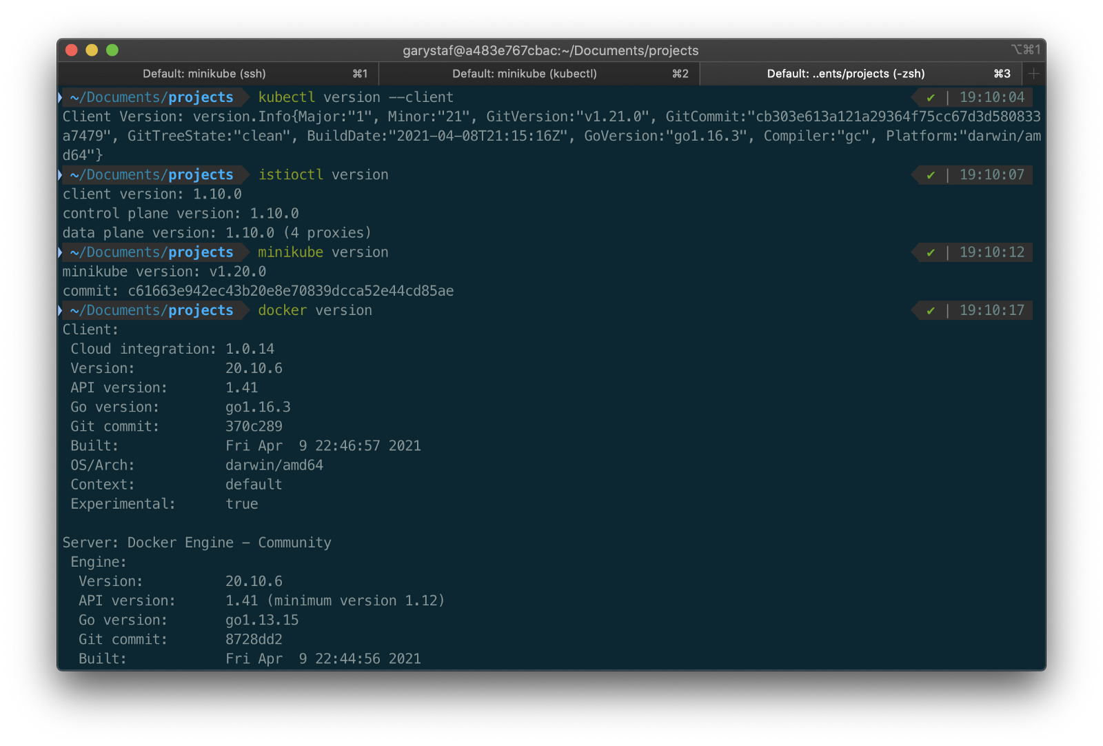
For this post demonstration, I am using an Apple MacBook Pro running macOS as my development machine. I have the latest versions of Docker Desktop, minikube, kubectl, and Istio installed as of May 2021.
Source Code
The source code for this post is open-source and is publicly available on GitHub. Clone the GitHub project using the following command:
clone --branch 2021-istio \
    --single-branch --depth 1 \
    https://github.com/garystafford/storefront-demo.git
Minikube
Part of the Kubernetes project, minikube is local Kubernetes, focusing on making it easy to learn and develop for Kubernetes. Minikube quickly sets up a local Kubernetes cluster on macOS, Linux, and Windows. Given the number of Kubernetes resources we will be deploying to minikube, I would recommend at least 3 CPUs and 4–5 GBs of memory. If you choose to deploy multiple observability tools, you may want to increase both of these resources if you can afford it. I maxed out both CPUs and memory several times while setting up this demonstration, causing temporary lock-ups of minikube.
minikube --cpus 3 --memory 5g --driver=docker start start

The Docker driver allows you to install Kubernetes into an existing Docker install. If you are using Docker, please be aware that you must have at least an equivalent amount of resources allocated to Docker to apportion to minikube.

Before continuing, confirm minikube is up and running and confirm the current context of kubectl is minikube.
minikube status
kubectl config current-context
The statuses should look similar to the following:

Use the eval below command to point your shell to minikube’s docker-daemon. You can confirm this by using the docker image ls and docker container ls command to view running Kubernetes containers on minikube.
eval $(minikube -p minikube docker-env)
docker image ls
docker container ls
The output should look similar to the following:

You can also check the status of minikube from Docker Desktop. Minikube is running as a container, instantiated from a Docker image, gcr.io/k8s-minikube/kicbase. View the container’s Stats, as shown below.

Istio
Assuming you have downloaded and configured Istio, install it onto minikube. I currently have Istio 1.10.0 installed and have theISTIO_HOME environment variable set in my Oh My Zsh .zshrc file. I have also set Istio’s bin/ subdirectory in my PATH environment variable. The bin/ subdirectory contains the istioctl executable.
echo $ISTIO_HOME
> /Applications/Istio/istio-1.10.0
where istioctl
> /Applications/Istio/istio-1.10.0/bin/istioctl
istioctl version

> client version: 1.10.0
  control plane version: 1.10.0
  data plane version: 1.10.0 (4 proxies)
Istio comes with several built-in configuration profiles. The profiles provide customization of the Istio control plane and of the sidecars for the Istio data plane.
istioctl profile list
> Istio configuration profiles:
    default
    demo
    empty
    external
    minimal
    openshift
    preview
    remote
For this demonstration, we will use the default profile, which installs istiod and an istio-ingressgateway. We will not require the use of an istio-egressgateway, since all components will be installed locally on minikube.
istioctl install --set profile=default -y
> ✔ Istio core installed
  ✔ Istiod installed
  ✔ Ingress gateways installed
  ✔ Installation complete

Minikube Tunnel
kubectl get svc istio-ingressgateway -n istio-system
To associate an IP address, run the minikube tunnel command in a separate terminal tab. Since it requires opening privileged ports 80 and 443 to be exposed, this command will prompt you for your sudo password.
Services of the type LoadBalancer can be exposed by using the minikube tunnel command. It must be run in a separate terminal window to keep the LoadBalancer running. We previously created the istio-ingressgateway. Run the following command and note that the status of EXTERNAL-IP is <pending>. There is currently no external IP address associated with our LoadBalancer.
minikube tunnel
Rerun the previous command. There should now be an external IP address associated with the LoadBalancer. In my case, 127.0.0.1.
kubectl get svc istio-ingressgateway -n istio-system
The external IP address shown is the address we will use to access the resources we chose to expose externally on minikube.
Minikube Dashboard
Once again, in a separate terminal tab, open the Minikube Dashboard (aka Kubernetes Dashboard).
minikube dashboard
The dashboard will give you a visual overview of all your installed Kubernetes components.

Namespaces
Kubernetes supports multiple virtual clusters backed by the same physical cluster. These virtual clusters are called namespaces. For this demonstration, we will use four namespaces to organize our deployed resources: dev, mongo, kafka, and storefront-kafka-project. The dev namespace is where we will deploy our Storefront API’s microservices: accounts, orders, and fulfillment. We will deploy MongoDB and Mongo Express to the mongo namespace. Lastly, we will use the kafka and storefront-kafka-project namespaces to deploy Apache Kafka to minikube using Strimzi, a Cloud Native Computing Foundation sandbox project, and CMAK.
kubectl apply -f ./minikube/resources/namespaces.yaml
Automatic Sidecar Injection
In order to take advantage of all of Istio’s features, pods in the mesh must be running an Istio sidecar proxy. When you set the istio-injection=enabled label on a namespace and the injection webhook is enabled, any new pods created in that namespace will automatically have a sidecar added to them. Labeling the dev namespace for automatic sidecar injection ensures that our Storefront API’s microservices — accounts, orders, and fulfillment— will have Istio sidecar proxy automatically injected into their pods.
kubectl label namespace dev istio-injection=enabled
MongoDB
Next, deploy MongoDB and Mongo Express to the mongo namespace on minikube. To ensure a successful connection to MongoDB from Mongo Express, I suggest giving MongoDB a chance to start up fully before deploying Mongo Express.
kubectl apply -f ./minikube/resources/mongodb.yaml -n mongo
sleep 60
kubectl apply -f ./minikube/resources/mongo-express.yaml -n mongo
To confirm the success of the deployments, use the following command:
kubectl get services -n mongo
Or use the Kubernetes Dashboard to confirm deployments.
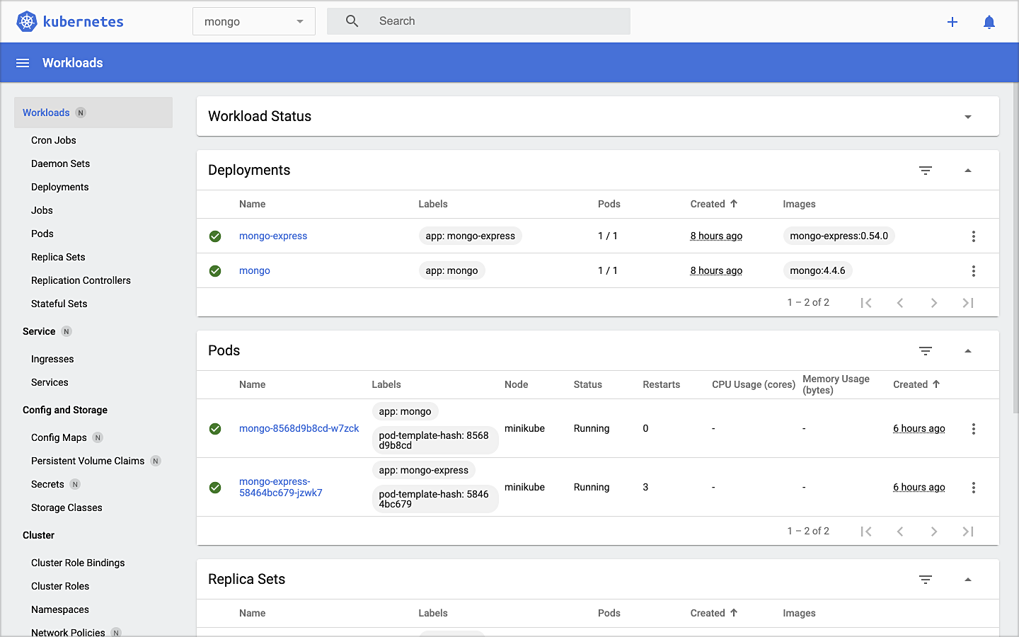
Mongo Express UI Access
For parts of your application (for example, frontends) you may want to expose a Service onto an external IP address outside of your cluster. Kubernetes ServiceTypes allows you to specify what kind of Service you want; the default is ClusterIP.
Note that while MongoDB uses the ClusterIP, Mongo Express uses NodePort. With NodePort, the Service is exposed on each Node’s IP at a static port (the NodePort). You can contact the NodePort Service, from outside the cluster, by requesting <NodeIP>:<NodePort>.
In a separate terminal tab, open Mongo Express using the following command:
minikube service --url mongo-express -n mongo
You should see output similar to the following:

Click on the link to open Mongo Express. There should already be three MongoDB operational databases shown in the UI. The three Storefront databases and collections will be created automatically, later in the post: accounts, orders, and fulfillment.

Apache Kafka using Strimzi
Next, we will install Apache Kafka and Apache Zookeeper into the kafka and storefront-kafka-project namespaces on minikube, using Strimzi. Since Strimzi has a great, easy-to-use Quick Start guide, I will not detail the complete install complete process in this post. I suggest using their guide to understand the process and what each command does. Then, use the slightly modified Strimzi commands I have included below to install Kafka and Zookeeper.
# assuming 0.23.0 is latest version available
curl -L -O https://github.com/strimzi/strimzi-kafka-operator/releases/download/0.23.0/strimzi-0.23.0.zip
unzip strimzi-0.23.0.zip
cd strimzi-0.23.0
sed -i '' 's/namespace: .*/namespace: kafka/' install/cluster-operator/*RoleBinding*.yaml
# manually change STRIMZI_NAMESPACE value to storefront-kafka-project
nano install/cluster-operator/060-Deployment-strimzi-cluster-operator.yaml
kubectl create -f install/cluster-operator/ -n kafka
kubectl create -f install/cluster-operator/020-RoleBinding-strimzi-cluster-operator.yaml -n storefront-kafka-project
kubectl create -f install/cluster-operator/032-RoleBinding-strimzi-cluster-operator-topic-operator-delegation.yaml -n storefront-kafka-project
kubectl create -f install/cluster-operator/031-RoleBinding-strimzi-cluster-operator-entity-operator-delegation.yaml -n storefront-kafka-project
kubectl apply -f ../storefront-demo/minikube/resources/strimzi-kafka-cluster.yaml -n storefront-kafka-project
kubectl wait kafka/kafka-cluster --for=condition=Ready --timeout=300s -n storefront-kafka-project
kubectl apply -f ../storefront-demo/minikube/resources/strimzi-kafka-topics.yaml -n storefront-kafka-project
Zoo Entrance
We want to install Yahoo’s CMAK (Cluster Manager for Apache Kafka) to give us a management interface for Kafka. However, CMAK required access to Zookeeper. You can not access Strimzi’s Zookeeper directly from CMAK; this is intentional to avoid performance and security issues. See this GitHub issue for a better explanation of why. We will use the appropriately named Zoo Entrance as a proxy for CMAK to Zookeeper to overcome this challenge.
To install Zoo Entrance, review the GitHub project’s install guide, then use the following commands:
git clone https://github.com/scholzj/zoo-entrance.git
cd zoo-entrance
# optional: change my-cluster to kafka-cluster
sed -i '' 's/my-cluster/kafka-cluster/' deploy.yaml
kubectl apply -f deploy.yaml -n storefront-kafka-project
Cluster Manager for Apache Kafka
Next, install Yahoo’s CMAK (Cluster Manager for Apache Kafka) to give us a management interface for Kafka. Run the following command to deploy CMAK into the storefront-kafka-project namespace.
kubectl apply -f ./minikube/resources/cmak.yaml -n storefront-kafka-project

Similar to Mongo Express, we can access CMAK’s UI using its NodePort. In a separate terminal tab, run the following command:
minikube service --url cmak -n storefront-kafka-project
You should see output similar to Mongo Express. Click on the link provided to access CMAK. Choose ‘Add Cluster’ in CMAK to add our existing Kafka cluster to CMAK’s management interface. Use Zoo Enterence’s service address for the Cluster Zookeeper Hosts value.
zoo-entrance.storefront-kafka-project.svc:2181

Once complete, you should see the three Kafka topics we created previously with Strimzi: accounts.customer.change, fulfillment.order.change, and orders.order.change. Each topic will have three partitions, one replica, and one broker. You should also see the _consumer_offsets topic that Kafka uses to store information about committed offsets for each topic:partition per group of consumers (groupID).

Storefront API Microservices
We are finally ready to install our Storefront API’s microservices into the dev namespace. Each service is preconfigured to access Kafka and MongoDB in their respective namespaces.
kubectl apply -f ./minikube/resources/accounts.yaml -n dev
kubectl apply -f ./minikube/resources/orders.yaml -n dev
kubectl apply -f ./minikube/resources/fulfillment.yaml -n dev
Spring Boot services usually take about two minutes to fully start. The time required to download the Docker Images from docker.com and the start-up time means it could take 3–4 minutes for each of the three services to be ready to accept API traffic.

Istio Components
We want to be able to access our Storefront API’s microservices through our Kubernetes LoadBalancer, while also leveraging all the capabilities of Istio as a service mesh. To do so, we need to deploy an Istio Gateway and a VirtualService. We will also need to deploy DestinationRule resources. A Gateway describes a load balancer operating at the edge of the mesh receiving incoming or outgoing HTTP/TCP connections. A VirtualService defines a set of traffic routing rules to apply when a host is addressed. Lastly, a DestinationRule defines policies that apply to traffic intended for a Service after routing has occurred.
kubectl apply -f ./minikube/resources/destination_rules.yaml -n dev
kubectl apply -f ./minikube/resources/istio-gateway.yaml -n dev
Testing the System and Creating Sample Data
I have provided a Python 3 script that runs a series of seven HTTP GET requests, in a specific order, against the Storefront API. These calls will validate the deployments, confirm the API’s services can access Kafka and MongoDB, generate some initial data, and automatically create the MongoDB database collections from the initial Insert statements.
python3 -m pip install -r ./utility_scripts/requirements.txt -U
python3 ./utility_scripts/refresh.py
The script’s output should be as follows:

If we now look at Mongo Express, we should note three new databases: accounts, orders, and fulfillment.

Observability Tools
Istio makes it easy to integrate with a number of common tools, including cert-manager, Prometheus, Grafana, Kiali, Zipkin, and Jaeger. In order to better observe our Storefront API, we will install three well-known observability tools: Kiali, Prometheus, and Grafana. Luckily, these tools are all included with Istio. You can install any or all of these to minikube. I suggest installing the tools one at a time as not to overwhelm minikube’s CPU and memory resources.
kubectl apply -f ./minikube/resources/prometheus.yaml

kubectl apply -f $ISTIO_HOME/samples/addons/grafana.yaml

kubectl apply -f $ISTIO_HOME/samples/addons/kiali.yaml
Once deployment is complete, to access any of the UI’s for these tools, use the istioctl dashboard command from a new terminal window:
istioctl dashboard kiali

istioctl dashboard prometheus

istioctl dashboard grafana
Kiali
Below we see a view of Kiali with API traffic flowing to Kafka and MongoDB.

Prometheus
Each of the three Storefront API microservices has a dependency on Micrometer; specifically, a dependency on micrometer-registry-prometheus. As an instrumentation facade, Micrometer allows you to instrument your code with dimensional metrics with a vendor-neutral interface and decide on the monitoring system as a last step. Instrumenting your core library code with Micrometer allows the libraries to be included in applications that ship metrics to different backends. Given the Micrometer Prometheus dependency, each microservice exposes a /prometheus endpoint (e.g., http://127.0.0.1/accounts/actuator/prometheus) as shown below in Postman.

The /prometheus endpoint exposes dozens of useful metrics and is configured to be scraped by Prometheus. These metrics can be displayed in Prometheus and indirectly in Grafana dashboards via Prometheus. I have customized Istio’s version of Prometheus and included it in the project (prometheus.yaml), which now scrapes the Storefront API’s metrics.
scrape_configs:
    - job_name: 'spring_micrometer'
      metrics_path: '/actuator/prometheus'
      scrape_interval: 5s
      static_configs:
        - targets: ['accounts.dev:8080','orders.dev:8080','fulfillment.dev:8080']
Here we see an example graph of a Spring Kafka Listener metric, spring_kafka_listener_seconds_sum, in Prometheus. There are dozens of metrics exposed to Prometheus from our system that we can observe and alert on.

Grafana
Lastly, here is an example Spring Boot Dashboard in Grafana. More dashboards are available on Grafana’s community dashboard page. The Grafana dashboard uses Prometheus as the source of its metrics data.

Storefront API Endpoints
The three storefront services are fully functional Spring Boot, Spring Data REST, Spring HATEOAS-enabled applications. Each service exposes a rich set of CRUD endpoints for interacting with the service’s data entities. To better understand the Storefront API, each Spring Boot microservice uses SpringFox, which produces automated JSON API documentation for APIs built with Spring. The service builds also include the springfox-swagger-ui web jar, which ships with Swagger UI. Swagger takes the manual work out of API documentation, with a range of solutions for generating, visualizing, and maintaining API docs.
From a web browser, you can use the /swagger-ui/ subdirectory/subpath with any of the three microservices to access the fully-featured Swagger UI (e.g., http://127.0.0.1/accounts/swagger-ui/).

Each service’s data model (POJOs) is also exposed through the Swagger UI.

Spring Boot Actuator
Additionally, each service includes Spring Boot Actuator. The Actuator exposes additional operational endpoints, allowing us to observe the running services. With Actuator, you get many features, including access to available operational-oriented endpoints, using the /actuator/ subdirectory/subpath (e.g., http://127.0.0.1/accounts/actuator/). For this demonstration, I have not restricted access to any available Actuator endpoints.


Conclusion
In this two-part post, we learned how to build an API using Spring Boot. We ensured the API’s distributed data integrity using a pub/sub model with Spring for Apache Kafka Project. When a relevant piece of data was changed by one microservice, that state change triggered a state change event that was shared with other microservices using Kafka topics.
We also learned how to deploy and run the API in a local development environment running on Kubernetes with Istio, using minikube. We have added production-tested observability tools to provide operational visibility, including CMAK, Mongo Express, Kiali, Prometheus, and Grafana.
This blog represents my own viewpoints and not of my employer, Amazon Web Services (AWS). All product names, logos, and brands are the property of their respective owners.
Eventual Consistency with Spring for Apache Kafka: Part 1 of 2
Posted by Gary A. Stafford in Bash Scripting, Java Development, Kubernetes, Software Development on May 22, 2021
Using Spring for Apache Kafka to manage a Distributed Data Model in MongoDB across multiple microservices
Given a modern distributed system composed of multiple microservices, each possessing a sub-set of a domain’s aggregate data, the system will almost assuredly have some data duplication. Given this duplication, how do we maintain data consistency? In this two-part post, we will explore one possible solution to this challenge — Apache Kafka and the model of eventual consistency.
Introduction
Apache Kafka is an open-source distributed event streaming platform capable of handling trillions of messages. According to Confluent, initially conceived as a messaging queue, Kafka is based on an abstraction of a distributed commit log. Since being created and open-sourced by LinkedIn in 2011, Kafka has quickly evolved from a messaging queue to a full-fledged event streaming platform.
Eventual consistency, according to Wikipedia, is a consistency model used in distributed computing to achieve high availability that informally guarantees that if no new updates are made to a given data item, eventually all accesses to that item will return the last updated value. I previously covered the topic of eventual consistency in a distributed system using RabbitMQ in the May 2017 post, Eventual Consistency: Decoupling Microservices with Spring AMQP and RabbitMQ. The post was featured on Pivotal’s RabbitMQ website.
Domain-driven Design
To ground the discussion, let’s examine a common example — an online storefront. Using a domain-driven design (DDD) approach, we would expect our problem domain, the online storefront, to be composed of multiple bounded contexts. Bounded contexts would likely include Shopping, Customer Service, Marketing, Security, Fulfillment, Accounting, and so forth, as shown in the context map, below.

Given this problem domain, we can assume we have the concept of a Customer. Further, we can assume the unique properties that define a Customer are likely to be spread across several bounded contexts. A complete view of the Customer will require you to aggregate data from multiple contexts. For example, the Accounting context may be the system of record for primary customer information, such as the customer’s name, contact information, contact preferences, and billing and shipping addresses. Marketing may possess additional information about the customer’s use of the store’s loyalty program and online shopping activity. Fulfillment may maintain a record of all orders being shipped to the customer. Security likely holds the customer’s access credentials, account access history, and privacy settings.
Below are the Customer data objects are shown in yellow. Orange represents the logical divisions of responsibility within each bounded context. These divisions will manifest themselves as individual microservices in our online storefront example.

Distributed Data Consistency
If we agree that the architecture of our domain’s data model requires some duplication of data across bounded contexts or even between services within the same context, then we must ensure data consistency. Take, for example, the case where a customer changes their home address or email. Let us assume that the Accounting context is the system of record for these data fields. However, to fulfill orders, the Shipping context might also need to maintain the customer’s current home address. Likewise, the Marketing context, responsible for opt-in email advertising, also needs to be aware of the email change and update its customer records.
If a piece of shared data is changed, then the party making the change should be responsible for communicating the change without expecting a response. They are stating a fact, not asking a question. Interested parties can choose if and how to act upon the change notification. This decoupled communication model is often described as Event-Carried State Transfer, defined by Martin Fowler of ThoughtWorks in his insightful post, What do you mean by “Event-Driven”?. Changes to a piece of data can be thought of as a state change event — events that contain details of the data that changed. Coincidentally, Fowler uses a customer’s address change as an example of Event-Carried State Transfer in the post. Fellow former ThoughtWorker Graham Brooks also detailed the concept in his post, Event-Carried State Transfer Pattern.
Consistency Strategies
Multiple architectural approaches can be taken to solve for data consistency in a distributed system. For example, you could use a single relational database with shared schemas to persist data, avoiding the distributed data model altogether. However, it could be argued that using a single database just turned your distributed system back into a monolith.
You could use Change Data Capture (CDC) to track changes to each database and send a record of those changes to Kafka topics for consumption by interested parties. Kafka Connect is an excellent choice for this, as explained in the article, No More Silos: How to Integrate your Databases with Apache Kafka and CDC, by Robin Moffatt of Confluent.
Alternately, we could use a separate data service, independent of the domain’s other business services, whose sole role is to ensure data consistency across domains. If messages persist in Kafka, the service has the added ability to provide data auditability through message replay. Of course, another set of services adds additional operational complexity to the system.
In this post’s somewhat simplistic architecture, the business microservices will maintain consistency across their respective domains by producing and consuming messages from multiple Kafka topics to which they are subscribed. Kafka Producers may also be Consumers within our domain.
Storefront Example
In this post, our online storefront API will be built in Java using Spring Boot and OpenJDK 16. We will ensure the uniformity of distributed data by using a publish/subscribe model with Spring for Apache Kafka Project. When a piece of data is changed by one Spring Boot microservice, if appropriate, that state change will trigger a state change event, which will be shared with other microservices using Kafka topics.

We will explore different methods of leveraging Spring Kafka to communicate state change events, as they relate to the specific use case of a customer placing an order through the online storefront. An abridged view of the storefront ordering process is shown in the diagram below. The arrows represent the exchange of data. Kafka will serve as a means of decoupling services from one another while still ensuring the data is distributed.

Given the use case of placing an order, we will examine the interactions of three services that compose our storefront API: the Accounts service within the Accounting bounded context, the Fulfillment service within the Fulfillment context, and the Orders service within the Order Management context. We will examine how the three services use Kafka to communicate state changes (changes to their data) to each other in a completely decoupled manner.
The diagram below shows the event flows between sub-systems discussed in the post. The numbering below corresponds to the numbering in the ordering process above. We will look at three event flows 2, 5, and 6. We will simulate event flow 3, the order being created by the Shopping Cart service.

Below is a view of the online storefront through the lens of the major sub-systems involved. Although the diagram is overly simplified, it should give you an idea of where Kafka and Zookeeper, Kafka’s current cluster manager, might sit in a typical, highly-available, microservice-based, distributed application platform.

This post will focus on the storefront’s backend API — its services, databases, and messaging sub-systems.

Storefront Microservices
We will explore the functionality of each of the three microservices and how they share state change events using Kafka 2.8. Each storefront API service is built using Spring Boot 2.0 and Gradle. Each Spring Boot service includes Spring Data REST, Spring Data MongoDB, Spring for Apache Kafka, Spring Cloud Sleuth, SpringFox, and Spring Boot Actuator. For simplicity, Kafka Streams and the use of Spring Cloud Stream are not part of this post.
Source Code
The storefront’s microservices source code is publicly available on GitHub. The four GitHub projects can be cloned using the following commands:
git clone --branch 2021-istio \
    --single-branch --depth 1 \
    https://github.com/garystafford/storefront-demo-accounts.git
git clone --branch 2021-istio \
    --single-branch --depth 1 \
    https://github.com/garystafford/storefront-demo-orders.git
git clone --branch 2021-istio \
    --single-branch --depth 1 \
    https://github.com/garystafford/storefront-demo-fulfillment.git
git clone --branch 2021-istio \
    --single-branch --depth 1 \
    https://github.com/garystafford/storefront-demo.git
Code samples in this post are displayed as Gists, which may not display correctly on some mobile and social media browsers. Links to gists are also provided.
Accounts Service
The Accounts service is responsible for managing basic customer information, such as name, contact information, addresses, and credit cards for purchases. A partial view of the data model for the Accounts service is shown below. This cluster of domain objects represents the Customer Account Aggregate.

The Customer class, the Accounts service’s primary data entity, is persisted in the Accounts MongoDB database. Below we see the representation of a Customer, as a BSON document in the customer.accounts MongoDB database collection.
Along with the primary Customer entity, the Accounts service contains a CustomerChangeEvent class. As a Kafka producer, the Accounts service uses the CustomerChangeEvent domain event object to carry state information about the client the Accounts service wishes to share when a new customer is added or a change is made to an existing customer. The CustomerChangeEvent object is not an exact duplicate of the Customer object. For example, the CustomerChangeEvent object does not share sensitive credit card information with other message Consumers (the CreditCard data object).

Since the CustomerChangeEvent domain event object does not persist in MongoDB, we can look at its JSON message payload in Kafka to examine its structure. Note the differences in the data structure (schema) between the Customer document in MongoDB and the Kafka CustomerChangeEvent message payload.
For simplicity, we will assume that other services do not make changes to the customer’s name, contact information, or addresses — this is the sole responsibility of the Accounts service.
Source code for the Accounts service is available on GitHub. Use the latest 2021-istio branch of the project.
Orders Service
The Orders service is responsible for managing a customer’s past and current orders; it is the system of record for the customer’s order history. A partial view of the data model for the Orders service is shown below. This cluster of domain objects represents the Customer Orders Aggregate.

The CustomerOrders class, the Order service’s primary data entity, is persisted in MongoDB. This entity contains a history of all the customer’s orders (Order data objects), along with the customer’s name, contact information, and addresses. In the Orders MongoDB database, a CustomerOrders, represented as a BSON document in the customer.orders database collection, looks as follows:
Along with the primary CustomerOrders entity, the Orders service contains the FulfillmentRequestEvent class. As a Kafka producer, the Orders service uses the FulfillmentRequestEvent domain event object to carry state information about an approved order, ready for fulfillment, which it sends to Kafka for consumption by the Fulfillment service. The FulfillmentRequestEvent object only contains the information it needs to share. Our example shares a single Order, along with the customer’s name, contact information, and shipping address.

Since the FulfillmentRequestEvent domain event object is not persisted in MongoDB, we can look at its JSON message payload in Kafka. Again, note the schema differences between the CustomerOrders document in MongoDB and the FulfillmentRequestEvent message payload in Kafka.
Source code for the Orders service is available on GitHub. Use the latest 2021-istio branch of the project.
Fulfillment Service
Lastly, the Fulfillment service is responsible for fulfilling orders. A partial view of the data model for the Fulfillment service is shown below. This cluster of domain objects represents the Fulfillment Aggregate.

The Fulfillment service’s primary entity, the Fulfillment class, is persisted in MongoDB. This entity contains a single Order data object, along with the customer’s name, contact information, and shipping address. The Fulfillment service also uses the Fulfillment entity to store the latest shipping status, such as ‘Shipped’, ‘In Transit’, and ‘Received’. The customer’s name, contact information, and shipping address are managed by the Accounts service, replicated to the Orders service, and passed to the Fulfillment service via Kafka, using the FulfillmentRequestEvent entity.
In the Fulfillment MongoDB database, a Fulfillment object represented as a BSON document in the fulfillment.requests database collection looks as follows:
Along with the primary Fulfillment entity, the Fulfillment service has an OrderStatusChangeEvent class. As a Kafka producer, the Fulfillment service uses the OrderStatusChangeEvent domain event object to carry state information about an order’s fulfillment statuses. The OrderStatusChangeEvent object contains the order’s UUID, a timestamp, shipping status, and an option for order status notes.
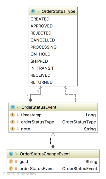
Since the OrderStatusChangeEvent domain event object is not persisted in MongoDB, again, we can again look at its JSON message payload in Kafka.
Source code for the Fulfillment service is available on GitHub. Use the latest 2021-istio branch of the project.
State Change Event Messaging Flows
There are three state change event messaging flows illustrated in this post.
- Changes to a Customer triggers an event message produced by the Accounts service, which is published on the
accounts.customer.changeKafka topic and consumed by the Orders service; - Order Approved triggers an event message produced by the Orders service, which is published on the
orders.order.fulfillKafka topic, and is consumed by the Fulfillment service; - Changes to the status of an Order triggers an event message produced by the Fulfillment Service, which is published on the
fulfillment.order.changeKafka topic, and is consumed by the Orders service;
Each of these state change event messaging flows follows the same architectural pattern on both the Kafka topic’s producer and consumer sides.

Let us examine each state change event messaging flow and the code behind it.
Customer State Change
When a new Customer entity is created or updated by the Accounts service, a CustomerChangeEvent message is produced and sent to the accounts.customer.change Kafka topic. This message is retrieved and consumed by the Orders service. This is how the Orders service eventually has a record of all customers who may place an order. By way of Kafka, it can be said that the Order’s Customer contact information is eventually consistent with the Account’s Customer contact information.

There are different methods to trigger a message to be sent to Kafka. For this particular state change, the Accounts service uses a listener. The listener class, which extends AbstractMongoEventListener, listens for an onAfterSave event for a Customer entity.
The listener handles the event by instantiating a new CustomerChangeEvent with the Customer’s information and passes it to the Sender class.
The SenderConfig class handles the configuration of the Sender. This Spring Kafka producer configuration class uses Spring Kafka’s JsonSerializer class to serialize the CustomerChangeEvent object into a JSON message payload.
The Sender uses a KafkaTemplate to send the message to the accounts.customer.change Kafka topic, as shown below. Since message order is critical to ensure changes to a Customer’s information are processed in order, all messages are sent to a single topic with a single partition.

The Orders service’s Receiver class consumes the CustomerChangeEvent messages produced by the Accounts service.
The Orders service’s Receiver class is configured differently compared to the Fulfillment service. The Orders service receives messages from multiple topics, each containing messages with different payload structures. Each type of message must be deserialized into different object types. To accomplish this, the ReceiverConfig class uses Apache Kafka’s StringDeserializer. The Orders service’s ReceiverConfig references Spring Kafka’s AbstractKafkaListenerContainerFactory classes setMessageConverter method, which allows for dynamic object type matching.
Each Kafka topic the Orders service consumes messages from is associated with a method in the Receiver class (shown above). This method accepts a specific object type as input, denoting the object type into which the message payload needs to be deserialized. This way, we can receive multiple message payloads, serialized from multiple object types, and successfully deserialize each type into the correct data object. In the case of a CustomerChangeEvent, the Orders service calls the receiveCustomerOrder method to consume the message and properly deserialize it.
For all services, a Spring application.yaml properties file in each service’s resources directory contains the Kafka configuration (lines 11–19).
Order Approved for Fulfillment
When the status of the Order in a CustomerOrders entity is changed to ‘Approved’ from ‘Created’, a FulfillmentRequestEvent message is produced and sent to the orders.order.fulfill Kafka topic. This message is retrieved and consumed by the Fulfillment service. This is how the Fulfillment service has a record of what Orders are ready for fulfillment.

Since we did not create the Shopping Cart service for this post, the Orders service simulates an order approval event, containing an approved order, being received, through Kafka, from the Shopping Cart Service. To simulate order creation and approval, the Orders service can create a random order history for each customer. Further, the Orders service can scan all customer orders for orders that contain both a ‘Created’ and ‘Approved’ order status. This state is communicated as an event message to Kafka for all orders matching those criteria. A FulfillmentRequestEvent is produced, which contains the order to be fulfilled, and the customer’s contact and shipping information. The FulfillmentRequestEvent is passed to the Sender class.
The SenderConfig class handles the configuration of the Sender class. This Spring Kafka producer configuration class uses Spring Kafka’s JsonSerializer class to serialize the FulfillmentRequestEvent object into a JSON message payload.
The Sender class uses a KafkaTemplate to send the message to the orders.order.fulfill Kafka topic, as shown below. Since message order is not critical, messages can be sent to a topic with multiple partitions if the volume of messages required it.

The Fulfillment service’s Receiver class consumes the FulfillmentRequestEvent from the Kafka topic and instantiates a Fulfillment object, containing the data passed in the FulfillmentRequestEvent message payload. The Fulfillment object includes the order to be fulfilled and the customer’s contact and shipping information.
The Fulfillment service’s ReceiverConfig class defines the DefaultKafkaConsumerFactory and ConcurrentKafkaListenerContainerFactory, responsible for deserializing the message payload from JSON into a FulfillmentRequestEvent object.
Fulfillment Order Status State Change
When the Order status in a Fulfillment entity is changed to anything other than Approved, an OrderStatusChangeEvent message is produced by the Fulfillment service and sent to the fulfillment.order.change Kafka topic. This message is retrieved and consumed by the Orders service. This is how the Orders service tracks all CustomerOrder lifecycle events from the initial Created status to the final Received status.

The Fulfillment service exposes several endpoints via the FulfillmentController class, which simulates a change in order status. They allow an order’s status to be changed from Approved to Processing, to Shipped, to In Transit, and finally to Received. This change applies to all orders that meet the criteria.
Each of these state changes triggers a change to the Fulfillment document in MongoDB. Each change also generates a Kafka message, containing the OrderStatusChangeEvent in the message payload. The Fulfillment service’s Sender class handles this.
Note in this example that these two events are not handled in an atomic transaction. Either updating the database or sending the message could fail independently, which would cause a loss of data consistency. In the real world, we must ensure that both these independent actions succeed or fail as a single transaction to ensure data consistency, using any of a handful of common architectural patterns.
The SenderConfig class handles the configuration of the Sender class. This Spring Kafka producer configuration class uses Spring Kafka’s JsonSerializer class to serialize the OrderStatusChangeEvent object into a JSON message payload. This class is almost identical to the SenderConfig class in the Orders and Accounts services.
The Sender class uses a KafkaTemplate to send the message to the fulfillment.order.change Kafka topic, as shown below. Message order is not critical since a timestamp is recorded, which ensures the proper sequence of order status events can be maintained. Messages can be sent to a topic with multiple partitions if the volume of messages requires it.

The Orders service’s Receiver class is responsible for consuming the OrderStatusChangeEvent message produced by the Fulfillment service.
As explained above, the Orders service is configured differently compared to the Fulfillment service, to receive messages from Kafka. The Orders service receives messages from more than one topic. The ReceiverConfig class deserializes all messages using the StringDeserializer. The Orders service’s ReceiverConfig class references the Spring Kafka AbstractKafkaListenerContainerFactory class’s setMessageConverter method, which allows for dynamic object type matching.
Each Kafka topic the Orders service consumes messages from is associated with a method in the Receiver class (shown above). This method accepts a specific object type as an input parameter, denoting the object type the message payload needs to be deserialized into. In the case of an OrderStatusChangeEvent message, the receiveOrderStatusChangeEvents method is called to consume a message from the fulfillment.order.change Kafka topic.
Part Two
In Part Two of this post, we will review how to deploy and run the storefront API components into a local development environment running on Kubernetes with Istio, using Minikube. To provide operational visibility, we will add observability tools, like Yahoo’s CMAK (Cluster Manager for Apache Kafka), Mongo Express, Kiali, Prometheus, and Grafana to our system.
This blog represents my own viewpoints and not of my employer, Amazon Web Services (AWS). All product names, logos, and brands are the property of their respective owners.
Using Eventual Consistency and Spring for Kafka to Manage a Distributed Data Model: Part 2
Posted by Gary A. Stafford in Enterprise Software Development, Java Development, Software Development on June 18, 2018
** This post has been rewritten and updated in May 2021 **
Given a modern distributed system, composed of multiple microservices, each possessing a sub-set of the domain’s aggregate data they need to perform their functions autonomously, we will almost assuredly have some duplication of data. Given this duplication, how do we maintain data consistency? In this two-part post, we’ve been exploring one possible solution to this challenge, using Apache Kafka and the model of eventual consistency. In Part One, we examined the online storefront domain, the storefront’s microservices, and the system’s state change event message flows.
Part Two
In Part Two of this post, I will briefly cover how to deploy and run a local development version of the storefront components, using Docker. The storefront’s microservices will be exposed through an API Gateway, Netflix’s Zuul. Service discovery and load balancing will be handled by Netflix’s Eureka. Both Zuul and Eureka are part of the Spring Cloud Netflix project. To provide operational visibility, we will add Yahoo’s Kafka Manager and Mongo Express to our system.

Source code for deploying the Dockerized components of the online storefront, shown in this post, is available on GitHub. All Docker Images are available on Docker Hub. I have chosen the wurstmeister/kafka-docker version of Kafka, available on Docker Hub; it has 580+ stars and 10M+ pulls on Docker Hub. This version of Kafka works well, as long as you run it within a Docker Swarm, locally.
Code samples in this post are displayed as Gists, which may not display correctly on some mobile and social media browsers. Links to gists are also provided.
Deployment Options
For simplicity, I’ve used Docker’s native Docker Swarm Mode to support the deployed online storefront. Docker requires minimal configuration as opposed to other CaaS platforms. Usually, I would recommend Minikube for local development if the final destination of the storefront were Kubernetes in Production (AKS, EKS, or GKE). Alternatively, if the final destination of the storefront was Red Hat OpenShift in Production, I would recommend Minishift for local development.
Docker Deployment
We will break up our deployment into two parts. First, we will deploy everything except our services. We will allow Kafka, MongoDB, Eureka, and the other components to start up fully. Afterward, we will deploy the three online storefront services. The storefront-kafka-docker project on Github contains two Docker Compose files, which are divided between the two tasks.
The middleware Docker Compose file (gist).
| version: '3.2' | |
| services: | |
| zuul: | |
| image: garystafford/storefront-zuul:latest | |
| expose: | |
| - "8080" | |
| ports: | |
| - "8080:8080/tcp" | |
| depends_on: | |
| - kafka | |
| - mongo | |
| - eureka | |
| hostname: zuul | |
| environment: | |
| # LOGGING_LEVEL_ROOT: DEBUG | |
| RIBBON_READTIMEOUT: 3000 | |
| RIBBON_SOCKETTIMEOUT: 3000 | |
| ZUUL_HOST_CONNECT_TIMEOUT_MILLIS: 3000 | |
| ZUUL_HOST_CONNECT_SOCKET_MILLIS: 3000 | |
| networks: | |
| - kafka-net | |
| eureka: | |
| image: garystafford/storefront-eureka:latest | |
| expose: | |
| - "8761" | |
| ports: | |
| - "8761:8761/tcp" | |
| hostname: eureka | |
| networks: | |
| - kafka-net | |
| mongo: | |
| image: mongo:latest | |
| command: --smallfiles | |
| # expose: | |
| # - "27017" | |
| ports: | |
| - "27017:27017/tcp" | |
| hostname: mongo | |
| networks: | |
| - kafka-net | |
| mongo_express: | |
| image: mongo-express:latest | |
| expose: | |
| - "8081" | |
| ports: | |
| - "8081:8081/tcp" | |
| hostname: mongo_express | |
| networks: | |
| - kafka-net | |
| zookeeper: | |
| image: wurstmeister/zookeeper:latest | |
| ports: | |
| - "2181:2181/tcp" | |
| hostname: zookeeper | |
| networks: | |
| - kafka-net | |
| kafka: | |
| image: wurstmeister/kafka:latest | |
| depends_on: | |
| - zookeeper | |
| # expose: | |
| # - "9092" | |
| ports: | |
| - "9092:9092/tcp" | |
| environment: | |
| KAFKA_ADVERTISED_HOST_NAME: kafka | |
| KAFKA_CREATE_TOPICS: "accounts.customer.change:1:1,fulfillment.order.change:1:1,orders.order.fulfill:1:1" | |
| KAFKA_ADVERTISED_PORT: 9092 | |
| KAFKA_ZOOKEEPER_CONNECT: zookeeper:2181 | |
| KAFKA_DELETE_TOPIC_ENABLE: "true" | |
| volumes: | |
| - /var/run/docker.sock:/var/run/docker.sock | |
| hostname: kafka | |
| networks: | |
| - kafka-net | |
| kafka_manager: | |
| image: hlebalbau/kafka-manager:latest | |
| ports: | |
| - "9000:9000/tcp" | |
| expose: | |
| - "9000" | |
| depends_on: | |
| - kafka | |
| environment: | |
| ZK_HOSTS: "zookeeper:2181" | |
| APPLICATION_SECRET: "random-secret" | |
| command: -Dpidfile.path=/dev/null | |
| hostname: kafka_manager | |
| networks: | |
| - kafka-net | |
| networks: | |
| kafka-net: | |
| driver: overlay |
The services Docker Compose file (gist).
| version: '3.2' | |
| services: | |
| accounts: | |
| image: garystafford/storefront-accounts:latest | |
| depends_on: | |
| - kafka | |
| - mongo | |
| hostname: accounts | |
| # environment: | |
| # LOGGING_LEVEL_ROOT: DEBUG | |
| networks: | |
| - kafka-net | |
| orders: | |
| image: garystafford/storefront-orders:latest | |
| depends_on: | |
| - kafka | |
| - mongo | |
| - eureka | |
| hostname: orders | |
| # environment: | |
| # LOGGING_LEVEL_ROOT: DEBUG | |
| networks: | |
| - kafka-net | |
| fulfillment: | |
| image: garystafford/storefront-fulfillment:latest | |
| depends_on: | |
| - kafka | |
| - mongo | |
| - eureka | |
| hostname: fulfillment | |
| # environment: | |
| # LOGGING_LEVEL_ROOT: DEBUG | |
| networks: | |
| - kafka-net | |
| networks: | |
| kafka-net: | |
| driver: overlay |
In the storefront-kafka-docker project, there is a shell script, stack_deploy_local.sh. This script will execute both Docker Compose files in succession, with a pause in between. You may need to adjust the timing for your own system (gist).
| #!/bin/sh | |
| # Deploys the storefront Docker stack | |
| # usage: sh ./stack_deploy_local.sh | |
| set -e | |
| docker stack deploy -c docker-compose-middleware.yml storefront | |
| echo "Starting the stack: middleware...pausing for 30 seconds..." | |
| sleep 30 | |
| docker stack deploy -c docker-compose-services.yml storefront | |
| echo "Starting the stack: services...pausing for 10 seconds..." | |
| sleep 10 | |
| docker stack ls | |
| docker stack services storefront | |
| docker container ls | |
| echo "Script completed..." | |
| echo "Services may take up to several minutes to start, fully..." |
Start by running docker swarm init. This command will initialize a Docker Swarm. Next, execute the stack deploy script, using an sh ./stack_deploy_local.sh command. The script will deploy a new Docker Stack, within the Docker Swarm. The Docker Stack will hold all storefront components, deployed as individual Docker containers. The stack is deployed within its own isolated Docker overlay network, kafka-net.
Note that we are not using host-based persistent storage for this local development demo. Destroying the Docker stack or the individual Kafka, Zookeeper, or MongoDB Docker containers will result in a loss of data.

Before completion, the stack deploy script runs docker stack ls command, followed by a docker stack services storefront command. You should see one stack, named storefront, with ten services. You should also see each of the ten services has 1/1 replicas running, indicating everything has started or is starting correctly, without failure. Failure would be reflected here as a service having 0/1 replicas.

Before completion, the stack deploy script also runs docker container ls command. You should observe each of the ten running containers (‘services’ in the Docker stack), along with their instance names and ports.

There is also a shell script, stack_delete_local.sh, which will issue a docker stack rm storefront command to destroy the stack when you are done.
Using the names of the storefront’s Docker containers, you can check the start-up logs of any of the components, using the docker logs command.

Testing the Stack
With the storefront stack deployed, we need to confirm that all the components have started correctly and are communicating with each other. To accomplish this, I’ve written a simple Python script, refresh.py. The refresh script has multiple uses. It deletes any existing storefront service MongoDB databases. It also deletes any existing Kafka topics; I call the Kafka Manager’s API to accomplish this. We have no databases or topics since our stack was just created. However, if you are actively developing your data models, you will likely want to purge the databases and topics regularly (gist).
| #!/usr/bin/env python3 | |
| # Delete (3) MongoDB databases, (3) Kafka topics, | |
| # create sample data by hitting Zuul API Gateway endpoints, | |
| # and return MongoDB documents as verification. | |
| # usage: python3 ./refresh.py | |
| from pprint import pprint | |
| from pymongo import MongoClient | |
| import requests | |
| import time | |
| client = MongoClient('mongodb://localhost:27017/') | |
| def main(): | |
| delete_databases() | |
| delete_topics() | |
| create_sample_data() | |
| get_mongo_doc('accounts', 'customer.accounts') | |
| get_mongo_doc('orders', 'customer.orders') | |
| get_mongo_doc('fulfillment', 'fulfillment.requests') | |
| def delete_databases(): | |
| dbs = ['accounts', 'orders', 'fulfillment'] | |
| for db in dbs: | |
| client.drop_database(db) | |
| print('MongoDB dropped: ' + db) | |
| dbs = client.database_names() | |
| print('Reamining databases:') | |
| print(dbs) | |
| print('\n') | |
| def delete_topics(): | |
| # call Kafka Manager API | |
| topics = ['accounts.customer.change', | |
| 'orders.order.fulfill', | |
| 'fulfillment.order.change'] | |
| for topic in topics: | |
| kafka_manager_url = 'http://localhost:9000/clusters/dev/topics/delete?t=' + topic | |
| r = requests.post(kafka_manager_url, data={'topic': topic}) | |
| time.sleep(3) | |
| print('Kafka topic deleted: ' + topic) | |
| print('\n') | |
| def create_sample_data(): | |
| sample_urls = [ | |
| 'http://localhost:8080/accounts/customers/sample', | |
| 'http://localhost:8080/orders/customers/sample/orders', | |
| 'http://localhost:8080/orders/customers/sample/fulfill', | |
| 'http://localhost:8080/fulfillment/fulfillments/sample/process', | |
| 'http://localhost:8080/fulfillment/fulfillments/sample/ship', | |
| 'http://localhost:8080/fulfillment/fulfillments/sample/in-transit', | |
| 'http://localhost:8080/fulfillment/fulfillments/sample/receive'%5D | |
| for sample_url in sample_urls: | |
| r = requests.get(sample_url) | |
| print(r.text) | |
| time.sleep(5) | |
| print('\n') | |
| def get_mongo_doc(db_name, collection_name): | |
| db = client[db_name] | |
| collection = db[collection_name] | |
| pprint(collection.find_one()) | |
| print('\n') | |
| if __name__ == "__main__": | |
| main() |
Next, the refresh script calls a series of RESTful HTTP endpoints, in a specific order, to create sample data. Our three storefront services each expose different endpoints. Different /sample endpoints create sample customers, orders, order fulfillment requests, and shipping notifications. The create sample data endpoints include, in order:
- Sample Customer: /accounts/customers/sample
- Sample Orders: /orders/customers/sample/orders
- Sample Fulfillment Requests: /orders/customers/sample/fulfill
- Sample Processed Order Events: /fulfillment/fulfillment/sample/process
- Sample Shipped Order Events: /fulfillment/fulfillment/sample/ship
- Sample In-Transit Order Events: /fulfillment/fulfillment/sample/in-transit
- Sample Received Order Events: /fulfillment/fulfillment/sample/receive
You can create data on your own by POSTing to the exposed CRUD endpoints on each service. However, given the complex data objects required in the request payloads, it is too time-consuming for this demo.
To execute the script, use a python3 ./refresh.py command. I am using Python 3 in the demo, but the script should also work with Python 2.x if you change shebang.

If everything was successful, the script returns one document from each of the three storefront service’s MongoDB database collections. A result of ‘None’ for any of the MongoDB documents usually indicates one of the earlier commands failed. Given an abnormally high response latency, due to the load of the ten running containers on my laptop, I had to increase the Zuul/Ribbon timeouts.
Observing the System
We should now have the online storefront Docker stack running, three MongoDB databases created and populated with sample documents (data), and three Kafka topics, which have messages in them. Based on the fact we saw database documents printed out with our refresh script, we know the topics were used to pass data between the message producing and message consuming services.
In most enterprise environments, a developer may not have the access, nor the operational knowledge to interact with Kafka or MongoDB from within a container, on the command line. So how else can we interact with the system?
Kafka Manager
Kafka Manager gives us the ability to interact with Kafka via a convenient browser-based user interface. For this demo, the Kafka Manager UI is available on the default port 9000.

To make Kafka Manager useful, define the Kafka cluster. The Cluster Name is up to you. The Cluster Zookeeper Host should be zookeeper:2181, for our demo.

Kafka Manager gives us useful insights into many aspects of our simple, single-broker cluster. You should observe three topics, created during the deployment of Kafka.

Kafka Manager is an appealing alternative, as opposed to connecting with the Kafka container, with a docker exec command, to interact with Kafka. A typical use case might be deleting a topic or adding partitions to a topic. We can also see which Consumers are consuming which topics, from within Kafka Manager.

Mongo Express
Similar to Kafka Manager, Mongo Express gives us the ability to interact with Kafka via a user interface. For this demo, the Mongo Express browser-based user interface is available on the default port 8081. The initial view displays each of the existing databases. Note our three service’s databases, including accounts, orders, and fulfillment.

Drilling into an individual database, we can view each of the database’s collections. Digging in further, we can interact with individual database collection documents.

We may even edit and save the documents.

SpringFox and Swagger
Each of the storefront services also implements SpringFox, the automated JSON API documentation for API’s built with Spring. With SpringFox, each service exposes a rich Swagger UI. The Swagger UI allows us to interact with service endpoints.
Since each service exposes its own Swagger interface, we must access them through the Zuul API Gateway on port 8080. In our demo environment, the Swagger browser-based user interface is accessible at /swagger-ui.html. Below is a fully self-documented Orders service API, as seen through the Swagger UI.
I believe there are still some incompatibilities with the latest SpringFox release and Spring Boot 2, which prevents Swagger from showing the default Spring Data REST CRUD endpoints. Currently, you only see the API endpoints you explicitly declare in your Controller classes.

The service’s data models (POJOs) are also exposed through the Swagger UI by default. Below we see the Orders service’s models.

The Swagger UI allows you to drill down into the complex structure of the models, such as the CustomerOrder entity, exposing each of the entity’s nested data objects.

Spring Cloud Netflix Eureka
This post does not cover the use of Eureka or Zuul. Eureka gives us further valuable insight into our storefront system. Eureka is our systems service registry and provides load-balancing for our services if we have multiple instances.
For this demo, the Eureka browser-based user interface is available on the default port 8761. Within the Eureka user interface, we should observe the three storefront services and Zuul, the API Gateway, registered with Eureka. If we had more than one instance of each service, we would see all of them listed here.

Although of limited use in a local environment, we can observe some general information about our host.

Interacting with the Services
The three storefront services are fully functional Spring Boot / Spring Data REST / Spring HATEOAS-enabled applications. Each service exposes a rich set of CRUD endpoints for interacting with the service’s data entities. Additionally, each service includes Spring Boot Actuator. Actuator exposes additional operational endpoints, allowing us to observe the running services. Again, this post is not intended to be a demonstration of Spring Boot or Spring Boot Actuator.
Using an application such as Postman, we can interact with our service’s RESTful HTTP endpoints. As shown below, we are calling the Account service’s customers resource. The Accounts request is proxied through the Zuul API Gateway.

The above Postman Storefront Collection and Postman Environment are both exported and saved with the project.
Some key endpoints to observe the entities that were created using Event-Carried State Transfer are shown below. They assume you are using localhost as a base URL.
- Zuul Registered Routes: /actuator/routes
- Accounts Service Customers: /accounts/customers
- Orders Service Customer Orders: /orders/customerOrderses
- Fulfillment Service Fulfillments: /fulfillment/fulfillments
References
Links to my GitHub projects for this post
- storefront-kafka-docker
- storefront-zuul-proxy
- storefront-eureka-server
- storefront-demo-accounts
- storefront-demo-orders
- storefront-demo-fulfillment
Some additional references I found useful while authoring this post and the online storefront code:
- Wurstmeister’s kafka-docker GitHub README
- Spring for Apache Kafka Reference Documentation
- Baeldung’s Intro to Apache Kafka with Spring
- CodeNotFound.com’s Spring Kafka – Consumer Producer Example
- MemoryNotFound’s Spring Kafka – Consumer and Producer Example
All opinions expressed in this post are my own and not necessarily the views of my current or past employers or their clients.
Using Eventual Consistency and Spring for Kafka to Manage a Distributed Data Model: Part 1
Posted by Gary A. Stafford in Enterprise Software Development, Java Development, Software Development on June 17, 2018
** This post has been rewritten and updated in May 2021 **
Given a modern distributed system, composed of multiple microservices, each possessing a sub-set of the domain’s aggregate data they need to perform their functions autonomously, we will almost assuredly have some duplication of data. Given this duplication, how do we maintain data consistency? In this two-part post, we will explore one possible solution to this challenge, using Apache Kafka and the model of eventual consistency.
I previously covered the topic of eventual consistency in a distributed system, using RabbitMQ, in the post, Eventual Consistency: Decoupling Microservices with Spring AMQP and RabbitMQ. This post is featured on Pivotal’s RabbitMQ website.
Introduction
To ground the discussion, let’s examine a common example of the online storefront. Using a domain-driven design (DDD) approach, we would expect our problem domain, the online storefront, to be composed of multiple bounded contexts. Bounded contexts would likely include Shopping, Customer Service, Marketing, Security, Fulfillment, Accounting, and so forth, as shown in the context map, below.

Given this problem domain, we can assume we have the concept of the Customer. Further, the unique properties that define a Customer are likely to be spread across several bounded contexts. A complete view of a Customer would require you to aggregate data from multiple contexts. For example, the Accounting context may be the system of record (SOR) for primary customer information, such as the customer’s name, contact information, contact preferences, and billing and shipping addresses. Marketing may possess additional information about the customer’s use of the store’s loyalty program. Fulfillment may maintain a record of all the orders shipped to the customer. Security likely holds the customer’s access credentials and privacy settings.
Below, Customer data objects are shown in yellow. Orange represents logical divisions of responsibility within each bounded context. These divisions will manifest themselves as individual microservices in our online storefront example. 
Distributed Data Consistency
If we agree that the architecture of our domain’s data model requires some duplication of data across bounded contexts, or even between services within the same contexts, then we must ensure data consistency. Take, for example, a change in a customer’s address. The Accounting context is the system of record for the customer’s addresses. However, to fulfill orders, the Shipping context might also need to maintain the customer’s address. Likewise, the Marketing context, who is responsible for direct-mail advertising, also needs to be aware of the address change, and update its own customer records.
If a piece of shared data is changed, then the party making the change should be responsible for communicating the change, without the expectation of a response. They are stating a fact, not asking a question. Interested parties can choose if, and how, to act upon the change notification. This decoupled communication model is often described as Event-Carried State Transfer, as defined by Martin Fowler, of ThoughtWorks, in his insightful post, What do you mean by “Event-Driven”?. A change to a piece of data can be thought of as a state change event. Coincidentally, Fowler also uses a customer’s address change as an example of Event-Carried State Transfer. The Event-Carried State Transfer Pattern is also detailed by fellow ThoughtWorker and noted Architect, Graham Brooks.
Consistency Strategies
Multiple architectural approaches could be taken to solve for data consistency in a distributed system. For example, you could use a single relational database to persist all data, avoiding the distributed data model altogether. Although I would argue, using a single database just turned your distributed system back into a monolith.
You could use Change Data Capture (CDC) to track changes to each database and send a record of those changes to Kafka topics for consumption by interested parties. Kafka Connect is an excellent choice for this, as explained in the article, No More Silos: How to Integrate your Databases with Apache Kafka and CDC, by Robin Moffatt of Confluent.
Alternately, we could use a separate data service, independent of the domain’s other business services, whose sole role is to ensure data consistency across domains. If messages are persisted in Kafka, the service have the added ability to provide data auditability through message replay. Of course, another set of services adds additional operational complexity.
Storefront Example
In this post, our online storefront’s services will be built using Spring Boot. Thus, we will ensure the uniformity of distributed data by using a Publish/Subscribe model with the Spring for Apache Kafka Project. When a piece of data is changed by one Spring Boot service, if appropriate, that state change will trigger an event, which will be shared with other services using Kafka topics.
We will explore different methods of leveraging Spring Kafka to communicate state change events, as they relate to the specific use case of a customer placing an order through the online storefront. An abridged view of the storefront ordering process is shown in the diagram below. The arrows represent the exchange of data. Kafka will serve as a means of decoupling services from each one another, while still ensuring the data is exchanged.

Given the use case of placing an order, we will examine the interactions of three services, the Accounts service within the Accounting bounded context, the Fulfillment service within the Fulfillment context, and the Orders service within the Order Management context. We will examine how the three services use Kafka to communicate state changes (changes to their data) to each other, in a decoupled manner.
The diagram below shows the event flows between sub-systems discussed in the post. The numbering below corresponds to the numbering in the ordering process above. We will look at event flows 2, 5, and 6. We will simulate event flow 3, the order being created by the Shopping Cart service. Kafka Producers may also be Consumers within our domain.

Below is a view of the online storefront, through the lens of the major sub-systems involved. Although the diagram is overly simplified, it should give you the idea of where Kafka, and Zookeeper, Kafka’s cluster manager, might sit in a typical, highly-available, microservice-based, distributed, application platform.

This post will focus on the storefront’s services, database, and messaging sub-systems.

Storefront Microservices
First, we will explore the functionality of each of the three microservices. We will examine how they share state change events using Kafka. Each storefront service is built using Spring Boot 2.0 and Gradle. Each Spring Boot service includes Spring Data REST, Spring Data MongoDB, Spring for Apache Kafka, Spring Cloud Sleuth, SpringFox, Spring Cloud Netflix Eureka, and Spring Boot Actuator. For simplicity, Kafka Streams and the use of Spring Cloud Stream is not part of this post.
Code samples in this post are displayed as Gists, which may not display correctly on some mobile and social media browsers. Links to gists are also provided.
Accounts Service
The Accounts service is responsible for managing basic customer information, such as name, contact information, addresses, and credit cards for purchases. A partial view of the data model for the Accounts service is shown below. This cluster of domain objects represents the Customer Account Aggregate.

The Customer class, the Accounts service’s primary data entity, is persisted in the Accounts MongoDB database. A Customer, represented as a BSON document in the customer.accounts database collection, looks as follows (gist).
| { | |
| "_id": ObjectId("5b189af9a8d05613315b0212"), | |
| "name": { | |
| "title": "Mr.", | |
| "firstName": "John", | |
| "middleName": "S.", | |
| "lastName": "Doe", | |
| "suffix": "Jr." | |
| }, | |
| "contact": { | |
| "primaryPhone": "555-666-7777", | |
| "secondaryPhone": "555-444-9898", | |
| "email": "john.doe@internet.com" | |
| }, | |
| "addresses": [{ | |
| "type": "BILLING", | |
| "description": "My cc billing address", | |
| "address1": "123 Oak Street", | |
| "city": "Sunrise", | |
| "state": "CA", | |
| "postalCode": "12345-6789" | |
| }, | |
| { | |
| "type": "SHIPPING", | |
| "description": "My home address", | |
| "address1": "123 Oak Street", | |
| "city": "Sunrise", | |
| "state": "CA", | |
| "postalCode": "12345-6789" | |
| } | |
| ], | |
| "creditCards": [{ | |
| "type": "PRIMARY", | |
| "description": "VISA", | |
| "number": "1234-6789-0000-0000", | |
| "expiration": "6/19", | |
| "nameOnCard": "John S. Doe" | |
| }, | |
| { | |
| "type": "ALTERNATE", | |
| "description": "Corporate American Express", | |
| "number": "9999-8888-7777-6666", | |
| "expiration": "3/20", | |
| "nameOnCard": "John Doe" | |
| } | |
| ], | |
| "_class": "com.storefront.model.Customer" | |
| } |
Along with the primary Customer entity, the Accounts service contains a CustomerChangeEvent class. As a Kafka producer, the Accounts service uses the CustomerChangeEvent domain event object to carry state information about the client the Accounts service wishes to share when a new customer is added, or a change is made to an existing customer. The CustomerChangeEvent object is not an exact duplicate of the Customer object. For example, the CustomerChangeEvent object does not share sensitive credit card information with other message Consumers (the CreditCard data object).

Since the CustomerChangeEvent domain event object is not persisted in MongoDB, to examine its structure, we can look at its JSON message payload in Kafka. Note the differences in the data structure between the Customer document in MongoDB and the Kafka CustomerChangeEvent message payload (gist).
| { | |
| "id": "5b189af9a8d05613315b0212", | |
| "name": { | |
| "title": "Mr.", | |
| "firstName": "John", | |
| "middleName": "S.", | |
| "lastName": "Doe", | |
| "suffix": "Jr." | |
| }, | |
| "contact": { | |
| "primaryPhone": "555-666-7777", | |
| "secondaryPhone": "555-444-9898", | |
| "email": "john.doe@internet.com" | |
| }, | |
| "addresses": [{ | |
| "type": "BILLING", | |
| "description": "My cc billing address", | |
| "address1": "123 Oak Street", | |
| "address2": null, | |
| "city": "Sunrise", | |
| "state": "CA", | |
| "postalCode": "12345-6789" | |
| }, { | |
| "type": "SHIPPING", | |
| "description": "My home address", | |
| "address1": "123 Oak Street", | |
| "address2": null, | |
| "city": "Sunrise", | |
| "state": "CA", | |
| "postalCode": "12345-6789" | |
| }] | |
| } |
For simplicity, we will assume other services do not make changes to the customer’s name, contact information, or addresses. It is the sole responsibility of the Accounts service.
Source code for the Accounts service is available on GitHub.
Orders Service
The Orders service is responsible for managing a customer’s past and current orders; it is the system of record for the customer’s order history. A partial view of the data model for the Orders service is shown below. This cluster of domain objects represents the Customer Orders Aggregate.

The CustomerOrders class, the Order service’s primary data entity, is persisted in MongoDB. This entity contains a history of all the customer’s orders (Order data objects), along with the customer’s name, contact information, and addresses. In the Orders MongoDB database, a CustomerOrders, represented as a BSON document in the customer.orders database collection, looks as follows (gist).
| { | |
| "_id": ObjectId("5b189af9a8d05613315b0212"), | |
| "name": { | |
| "title": "Mr.", | |
| "firstName": "John", | |
| "middleName": "S.", | |
| "lastName": "Doe", | |
| "suffix": "Jr." | |
| }, | |
| "contact": { | |
| "primaryPhone": "555-666-7777", | |
| "secondaryPhone": "555-444-9898", | |
| "email": "john.doe@internet.com" | |
| }, | |
| "addresses": [{ | |
| "type": "BILLING", | |
| "description": "My cc billing address", | |
| "address1": "123 Oak Street", | |
| "city": "Sunrise", | |
| "state": "CA", | |
| "postalCode": "12345-6789" | |
| }, | |
| { | |
| "type": "SHIPPING", | |
| "description": "My home address", | |
| "address1": "123 Oak Street", | |
| "city": "Sunrise", | |
| "state": "CA", | |
| "postalCode": "12345-6789" | |
| } | |
| ], | |
| "orders": [{ | |
| "guid": "df78784f-4d1d-48ad-a3e3-26a4fe7317a4", | |
| "orderStatusEvents": [{ | |
| "timestamp": NumberLong("1528339278058"), | |
| "orderStatusType": "CREATED" | |
| }, | |
| { | |
| "timestamp": NumberLong("1528339278058"), | |
| "orderStatusType": "APPROVED" | |
| }, | |
| { | |
| "timestamp": NumberLong("1528339278058"), | |
| "orderStatusType": "PROCESSING" | |
| }, | |
| { | |
| "timestamp": NumberLong("1528339278058"), | |
| "orderStatusType": "COMPLETED" | |
| } | |
| ], | |
| "orderItems": [{ | |
| "product": { | |
| "guid": "7f3c9c22-3c0a-47a5-9a92-2bd2e23f6e37", | |
| "title": "Green Widget", | |
| "description": "Gorgeous Green Widget", | |
| "price": "11.99" | |
| }, | |
| "quantity": 2 | |
| }, | |
| { | |
| "product": { | |
| "guid": "d01fde07-7c24-49c5-a5f1-bc2ce1f14c48", | |
| "title": "Red Widget", | |
| "description": "Reliable Red Widget", | |
| "price": "3.99" | |
| }, | |
| "quantity": 3 | |
| } | |
| ] | |
| }, | |
| { | |
| "guid": "29692d7f-3ca5-4684-b5fd-51dbcf40dc1e", | |
| "orderStatusEvents": [{ | |
| "timestamp": NumberLong("1528339278058"), | |
| "orderStatusType": "CREATED" | |
| }, | |
| { | |
| "timestamp": NumberLong("1528339278058"), | |
| "orderStatusType": "APPROVED" | |
| } | |
| ], | |
| "orderItems": [{ | |
| "product": { | |
| "guid": "a9d5a5c7-4245-4b4e-b1c3-1d3968f36b2d", | |
| "title": "Yellow Widget", | |
| "description": "Amazing Yellow Widget", | |
| "price": "5.99" | |
| }, | |
| "quantity": 1 | |
| }] | |
| } | |
| ], | |
| "_class": "com.storefront.model.CustomerOrders" | |
| } |
Along with the primary CustomerOrders entity, the Orders service contains the FulfillmentRequestEvent class. As a Kafka producer, the Orders service uses the FulfillmentRequestEvent domain event object to carry state information about an approved order, ready for fulfillment, which it sends to Kafka for consumption by the Fulfillment service. TheFulfillmentRequestEvent object only contains the information it needs to share. In our example, it shares a single Order, along with the customer’s name, contact information, and shipping address.

Since the FulfillmentRequestEvent domain event object is not persisted in MongoDB, we can look at it’s JSON message payload in Kafka. Again, note the structural differences between the CustomerOrders document in MongoDB and the FulfillmentRequestEvent message payload in Kafka (gist).
| { | |
| "timestamp": 1528334218821, | |
| "name": { | |
| "title": "Mr.", | |
| "firstName": "John", | |
| "middleName": "S.", | |
| "lastName": "Doe", | |
| "suffix": "Jr." | |
| }, | |
| "contact": { | |
| "primaryPhone": "555-666-7777", | |
| "secondaryPhone": "555-444-9898", | |
| "email": "john.doe@internet.com" | |
| }, | |
| "address": { | |
| "type": "SHIPPING", | |
| "description": "My home address", | |
| "address1": "123 Oak Street", | |
| "address2": null, | |
| "city": "Sunrise", | |
| "state": "CA", | |
| "postalCode": "12345-6789" | |
| }, | |
| "order": { | |
| "guid": "facb2d0c-4ae7-4d6c-96a0-293d9c521652", | |
| "orderStatusEvents": [{ | |
| "timestamp": 1528333926586, | |
| "orderStatusType": "CREATED", | |
| "note": null | |
| }, { | |
| "timestamp": 1528333926586, | |
| "orderStatusType": "APPROVED", | |
| "note": null | |
| }], | |
| "orderItems": [{ | |
| "product": { | |
| "guid": "7f3c9c22-3c0a-47a5-9a92-2bd2e23f6e37", | |
| "title": "Green Widget", | |
| "description": "Gorgeous Green Widget", | |
| "price": 11.99 | |
| }, | |
| "quantity": 5 | |
| }] | |
| } | |
| } |
Source code for the Orders service is available on GitHub.
Fulfillment Service
Lastly, the Fulfillment service is responsible for fulfilling orders. A partial view of the data model for the Fulfillment service is shown below. This cluster of domain objects represents the Fulfillment Aggregate.

The Fulfillment service’s primary entity, the Fulfillment class, is persisted in MongoDB. This entity contains a single Order data object, along with the customer’s name, contact information, and shipping address. The Fulfillment service also uses the Fulfillment entity to store the latest shipping event, such as ‘Shipped’, ‘In Transit’, and ‘Received’. The customer’s name, contact information, and shipping addresses are managed by the Accounts service, replicated to the Orders service, and passed to the Fulfillment service, via Kafka, using the FulfillmentRequestEvent entity.
In the Fulfillment MongoDB database, a Fulfillment object, represented as a BSON document in the fulfillment.requests database collection, looks as follows (gist).
| { | |
| "_id": ObjectId("5b1bf1b8a8d0562de5133d64"), | |
| "timestamp": NumberLong("1528553706260"), | |
| "name": { | |
| "title": "Ms.", | |
| "firstName": "Susan", | |
| "lastName": "Blackstone" | |
| }, | |
| "contact": { | |
| "primaryPhone": "433-544-6555", | |
| "secondaryPhone": "223-445-6767", | |
| "email": "susan.m.blackstone@emailisus.com" | |
| }, | |
| "address": { | |
| "type": "SHIPPING", | |
| "description": "Home Sweet Home", | |
| "address1": "33 Oak Avenue", | |
| "city": "Nowhere", | |
| "state": "VT", | |
| "postalCode": "444556-9090" | |
| }, | |
| "order": { | |
| "guid": "2932a8bf-aa9c-4539-8cbf-133a5bb65e44", | |
| "orderStatusEvents": [{ | |
| "timestamp": NumberLong("1528558453686"), | |
| "orderStatusType": "RECEIVED" | |
| }], | |
| "orderItems": [{ | |
| "product": { | |
| "guid": "4efe33a1-722d-48c8-af8e-7879edcad2fa", | |
| "title": "Purple Widget" | |
| }, | |
| "quantity": 2 | |
| }, | |
| { | |
| "product": { | |
| "guid": "b5efd4a0-4eb9-4ad0-bc9e-2f5542cbe897", | |
| "title": "Blue Widget" | |
| }, | |
| "quantity": 5 | |
| }, | |
| { | |
| "product": { | |
| "guid": "a9d5a5c7-4245-4b4e-b1c3-1d3968f36b2d", | |
| "title": "Yellow Widget" | |
| }, | |
| "quantity": 2 | |
| } | |
| ] | |
| }, | |
| "shippingMethod": "Drone", | |
| "_class": "com.storefront.model.Fulfillment" | |
| } |
Along with the primary Fulfillment entity, the Fulfillment service has an OrderStatusChangeEvent class. As a Kafka producer, the Fulfillment service uses the OrderStatusChangeEvent domain event object to carry state information about an order’s fulfillment statuses. The OrderStatusChangeEvent object contains the order’s UUID, a timestamp, shipping status, and an option for order status notes.

Since the OrderStatusChangeEvent domain event object is not persisted in MongoDB, to examine it, we can again look at it’s JSON message payload in Kafka (gist).
| { | |
| "guid": "facb2d0c-4ae7-4d6c-96a0-293d9c521652", | |
| "orderStatusEvent": { | |
| "timestamp": 1528334452746, | |
| "orderStatusType": "PROCESSING", | |
| "note": null | |
| } | |
| } |
Source code for the Fulfillment service is available on GitHub.
State Change Event Messaging Flows
There are three state change event messaging flows demonstrated in this post.
- Change to a Customer triggers an event message by the Accounts service;
- Order Approved triggers an event message by the Orders service;
- Change to the status of an Order triggers an event message by the Fulfillment service;
Each of these state change event messaging flows follow the exact same architectural pattern on both the Producer and Consumer sides of the Kafka topic.

Let’s examine each state change event messaging flow and the code behind them.
Customer State Change
When a new Customer entity is created or updated by the Accounts service, a CustomerChangeEvent message is produced and sent to the accounts.customer.change Kafka topic. This message is retrieved and consumed by the Orders service. This is how the Orders service eventually has a record of all customers who may place an order. It can be said that the Order’s Customer contact information is eventually consistent with the Account’s Customer contact information, by way of Kafka.

There are different methods to trigger a message to be sent to Kafka, For this particular state change, the Accounts service uses a listener. The listener class, which extends AbstractMongoEventListener, listens for an onAfterSave event for a Customer entity (gist).
| @Slf4j | |
| @Controller | |
| public class AfterSaveListener extends AbstractMongoEventListener<Customer> { | |
| @Value("${spring.kafka.topic.accounts-customer}") | |
| private String topic; | |
| private Sender sender; | |
| @Autowired | |
| public AfterSaveListener(Sender sender) { | |
| this.sender = sender; | |
| } | |
| @Override | |
| public void onAfterSave(AfterSaveEvent<Customer> event) { | |
| log.info("onAfterSave event='{}'", event); | |
| Customer customer = event.getSource(); | |
| CustomerChangeEvent customerChangeEvent = new CustomerChangeEvent(); | |
| customerChangeEvent.setId(customer.getId()); | |
| customerChangeEvent.setName(customer.getName()); | |
| customerChangeEvent.setContact(customer.getContact()); | |
| customerChangeEvent.setAddresses(customer.getAddresses()); | |
| sender.send(topic, customerChangeEvent); | |
| } | |
| } |
The listener handles the event by instantiating a new CustomerChangeEvent with the Customer’s information and passes it to the Sender class (gist).
| @Slf4j | |
| public class Sender { | |
| @Autowired | |
| private KafkaTemplate<String, CustomerChangeEvent> kafkaTemplate; | |
| public void send(String topic, CustomerChangeEvent payload) { | |
| log.info("sending payload='{}' to topic='{}'", payload, topic); | |
| kafkaTemplate.send(topic, payload); | |
| } | |
| } |
The configuration of the Sender is handled by the SenderConfig class. This Spring Kafka producer configuration class uses Spring Kafka’s JsonSerializer class to serialize the CustomerChangeEvent object into a JSON message payload (gist).
| @Configuration | |
| @EnableKafka | |
| public class SenderConfig { | |
| @Value("${spring.kafka.bootstrap-servers}") | |
| private String bootstrapServers; | |
| @Bean | |
| public Map<String, Object> producerConfigs() { | |
| Map<String, Object> props = new HashMap<>(); | |
| props.put(ProducerConfig.BOOTSTRAP_SERVERS_CONFIG, bootstrapServers); | |
| props.put(ProducerConfig.KEY_SERIALIZER_CLASS_CONFIG, StringSerializer.class); | |
| props.put(ProducerConfig.VALUE_SERIALIZER_CLASS_CONFIG, JsonSerializer.class); | |
| return props; | |
| } | |
| @Bean | |
| public ProducerFactory<String, CustomerChangeEvent> producerFactory() { | |
| return new DefaultKafkaProducerFactory<>(producerConfigs()); | |
| } | |
| @Bean | |
| public KafkaTemplate<String, CustomerChangeEvent> kafkaTemplate() { | |
| return new KafkaTemplate<>(producerFactory()); | |
| } | |
| @Bean | |
| public Sender sender() { | |
| return new Sender(); | |
| } | |
| } |
The Sender uses a KafkaTemplate to send the message to the Kafka topic, as shown below. Since message order is critical to ensure changes to a Customer’s information are processed in order, all messages are sent to a single topic with a single partition.
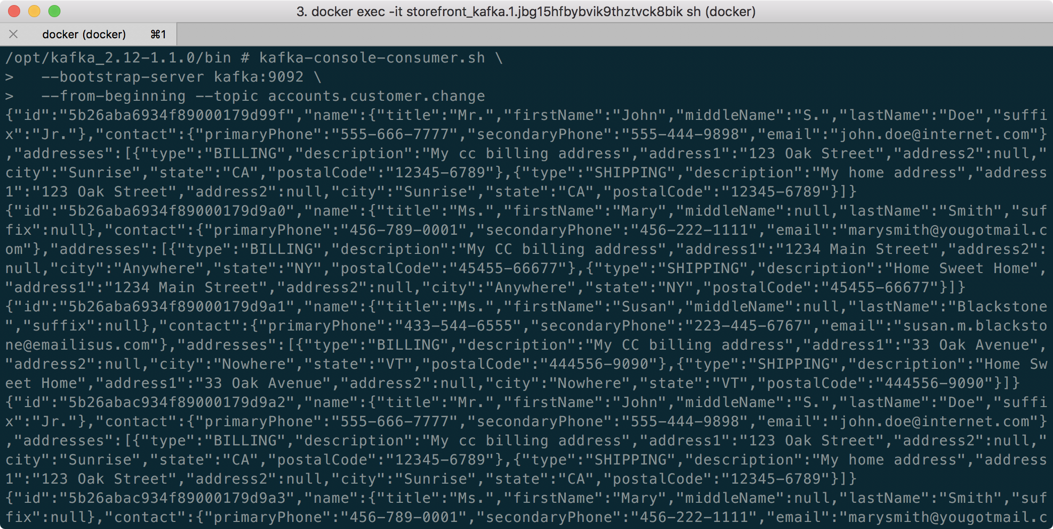
The Orders service’s Receiver class consumes the CustomerChangeEvent messages, produced by the Accounts service (gist).
[gust]cc3c4e55bc291e5435eccdd679d03015[/gist]
The Orders service’s Receiver class is configured differently, compared to the Fulfillment service. The Orders service receives messages from multiple topics, each containing messages with different payload structures. Each type of message must be deserialized into different object types. To accomplish this, the ReceiverConfig class uses Apache Kafka’s StringDeserializer. The Orders service’s ReceiverConfig references Spring Kafka’s AbstractKafkaListenerContainerFactory classes setMessageConverter method, which allows for dynamic object type matching (gist).
| @Configuration | |
| @EnableKafka | |
| public class ReceiverConfigNotConfluent implements ReceiverConfig { | |
| @Value("${spring.kafka.bootstrap-servers}") | |
| private String bootstrapServers; | |
| @Value("${spring.kafka.consumer.group-id}") | |
| private String groupId; | |
| @Value("${spring.kafka.consumer.auto-offset-reset}") | |
| private String autoOffsetReset; | |
| @Override | |
| @Bean | |
| public Map<String, Object> consumerConfigs() { | |
| Map<String, Object> props = new HashMap<>(); | |
| props.put(ProducerConfig.BOOTSTRAP_SERVERS_CONFIG, bootstrapServers); | |
| props.put(ConsumerConfig.KEY_DESERIALIZER_CLASS_CONFIG, StringDeserializer.class); | |
| props.put(ConsumerConfig.VALUE_DESERIALIZER_CLASS_CONFIG, StringDeserializer.class); | |
| props.put(ConsumerConfig.GROUP_ID_CONFIG, groupId); | |
| props.put(ConsumerConfig.AUTO_OFFSET_RESET_CONFIG, autoOffsetReset); | |
| return props; | |
| } | |
| @Override | |
| @Bean | |
| public ConsumerFactory<String, String> consumerFactory() { | |
| return new DefaultKafkaConsumerFactory<>(consumerConfigs(), | |
| new StringDeserializer(), | |
| new StringDeserializer() | |
| ); | |
| } | |
| @Bean | |
| ConcurrentKafkaListenerContainerFactory<String, String> kafkaListenerContainerFactory() { | |
| ConcurrentKafkaListenerContainerFactory<String, String> factory = | |
| new ConcurrentKafkaListenerContainerFactory<>(); | |
| factory.setConsumerFactory(consumerFactory()); | |
| factory.setMessageConverter(new StringJsonMessageConverter()); | |
| return factory; | |
| } | |
| @Override | |
| @Bean | |
| public Receiver receiver() { | |
| return new Receiver(); | |
| } | |
| } |
Each Kafka topic the Orders service consumes messages from is associated with a method in the Receiver class (shown above). That method accepts a specific object type as input, denoting the object type the message payload needs to be deserialized into. In this way, we can receive multiple message payloads, serialized from multiple object types, and successfully deserialize each type into the correct data object. In the case of a CustomerChangeEvent, the Orders service calls the receiveCustomerOrder method to consume the message and properly deserialize it.
For all services, a Spring application.yaml properties file, in each service’s resources directory, contains the Kafka configuration (gist).
| server: | |
| port: 8080 | |
| spring: | |
| main: | |
| allow-bean-definition-overriding: true | |
| application: | |
| name: orders | |
| data: | |
| mongodb: | |
| uri: mongodb://mongo:27017/orders | |
| kafka: | |
| bootstrap-servers: kafka:9092 | |
| topic: | |
| accounts-customer: accounts.customer.change | |
| orders-order: orders.order.fulfill | |
| fulfillment-order: fulfillment.order.change | |
| consumer: | |
| group-id: orders | |
| auto-offset-reset: earliest | |
| zipkin: | |
| sender: | |
| type: kafka | |
| management: | |
| endpoints: | |
| web: | |
| exposure: | |
| include: '*' | |
| logging: | |
| level: | |
| root: INFO | |
| --- | |
| spring: | |
| config: | |
| activate: | |
| on-profile: local | |
| data: | |
| mongodb: | |
| uri: mongodb://localhost:27017/orders | |
| kafka: | |
| bootstrap-servers: localhost:9092 | |
| server: | |
| port: 8090 | |
| management: | |
| endpoints: | |
| web: | |
| exposure: | |
| include: '*' | |
| logging: | |
| level: | |
| root: DEBUG | |
| --- | |
| spring: | |
| config: | |
| activate: | |
| on-profile: confluent | |
| server: | |
| port: 8080 | |
| logging: | |
| level: | |
| root: INFO | |
| --- | |
| server: | |
| port: 8080 | |
| spring: | |
| config: | |
| activate: | |
| on-profile: minikube | |
| data: | |
| mongodb: | |
| uri: mongodb://mongo.dev:27017/orders | |
| kafka: | |
| bootstrap-servers: kafka-cluster.dev:9092 | |
| management: | |
| endpoints: | |
| web: | |
| exposure: | |
| include: '*' | |
| logging: | |
| level: | |
| root: DEBUG |
Order Approved for Fulfillment
When the status of the Order in a CustomerOrders entity is changed to ‘Approved’ from ‘Created’, a FulfillmentRequestEvent message is produced and sent to the accounts.customer.change Kafka topic. This message is retrieved and consumed by the Fulfillment service. This is how the Fulfillment service has a record of what Orders are ready for fulfillment.

Since we did not create the Shopping Cart service for this post, the Orders service simulates an order approval event, containing an approved order, being received, through Kafka, from the Shopping Cart Service. To simulate order creation and approval, the Orders service can create a random order history for each customer. Further, the Orders service can scan all customer orders for orders that contain both a ‘Created’ and ‘Approved’ order status. This state is communicated as an event message to Kafka for all orders matching those criteria. A FulfillmentRequestEvent is produced, which contains the order to be fulfilled, and the customer’s contact and shipping information. The FulfillmentRequestEvent is passed to the Sender class (gist).
| @Slf4j | |
| public class Sender { | |
| @Autowired | |
| private KafkaTemplate<String, FulfillmentRequestEvent> kafkaTemplate; | |
| public void send(String topic, FulfillmentRequestEvent payload) { | |
| log.info("sending payload='{}' to topic='{}'", payload, topic); | |
| kafkaTemplate.send(topic, payload); | |
| } | |
| } |
The configuration of the Sender class is handled by the SenderConfig class. This Spring Kafka producer configuration class uses the Spring Kafka’s JsonSerializer class to serialize the FulfillmentRequestEvent object into a JSON message payload (gist).
| @Configuration | |
| @EnableKafka | |
| public class SenderConfig { | |
| @Value("${spring.kafka.bootstrap-servers}") | |
| private String bootstrapServers; | |
| @Bean | |
| public Map<String, Object> producerConfigs() { | |
| Map<String, Object> props = new HashMap<>(); | |
| props.put(ProducerConfig.BOOTSTRAP_SERVERS_CONFIG, bootstrapServers); | |
| props.put(ProducerConfig.KEY_SERIALIZER_CLASS_CONFIG, StringSerializer.class); | |
| props.put(ProducerConfig.VALUE_SERIALIZER_CLASS_CONFIG, JsonSerializer.class); | |
| return props; | |
| } | |
| @Bean | |
| public ProducerFactory<String, FulfillmentRequestEvent> producerFactory() { | |
| return new DefaultKafkaProducerFactory<>(producerConfigs()); | |
| } | |
| @Bean | |
| public KafkaTemplate<String, FulfillmentRequestEvent> kafkaTemplate() { | |
| return new KafkaTemplate<>(producerFactory()); | |
| } | |
| @Bean | |
| public Sender sender() { | |
| return new Sender(); | |
| } | |
| } |
The Sender class uses a KafkaTemplate to send the message to the Kafka topic, as shown below. Since message order is not critical messages could be sent to a topic with multiple partitions if the volume of messages required it.
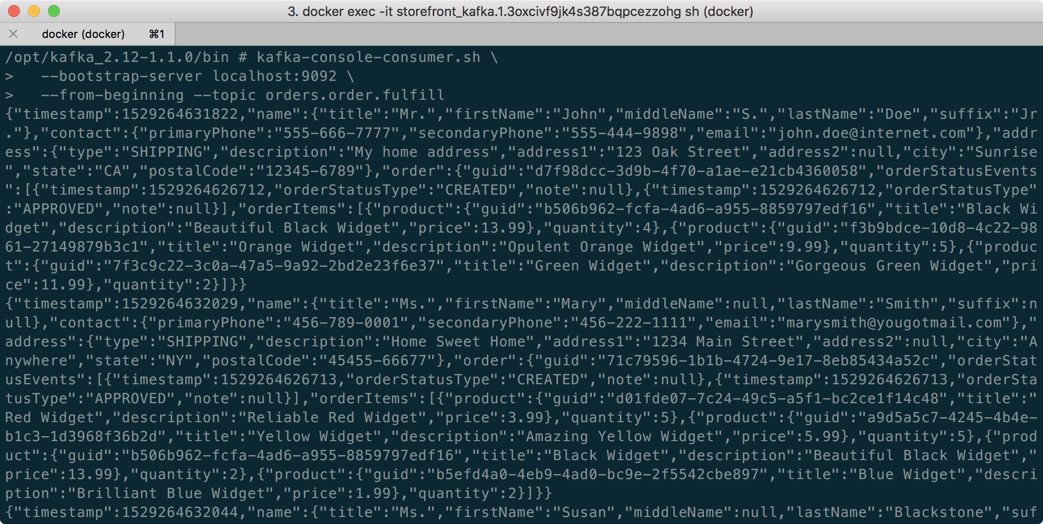
The Fulfillment service’s Receiver class consumes the FulfillmentRequestEvent from the Kafka topic and instantiates a Fulfillment object, containing the data passed in the FulfillmentRequestEvent message payload. This includes the order to be fulfilled and the customer’s contact and shipping information (gist).
| @Slf4j | |
| @Component | |
| public class Receiver { | |
| @Autowired | |
| private FulfillmentRepository fulfillmentRepository; | |
| private CountDownLatch latch = new CountDownLatch(1); | |
| public CountDownLatch getLatch() { | |
| return latch; | |
| } | |
| @KafkaListener(topics = "${spring.kafka.topic.orders-order}") | |
| public void receive(FulfillmentRequestEvent fulfillmentRequestEvent) { | |
| log.info("received payload='{}'", fulfillmentRequestEvent.toString()); | |
| latch.countDown(); | |
| Fulfillment fulfillment = new Fulfillment(); | |
| fulfillment.setId(fulfillmentRequestEvent.getId()); | |
| fulfillment.setTimestamp(fulfillmentRequestEvent.getTimestamp()); | |
| fulfillment.setName(fulfillmentRequestEvent.getName()); | |
| fulfillment.setContact(fulfillmentRequestEvent.getContact()); | |
| fulfillment.setAddress(fulfillmentRequestEvent.getAddress()); | |
| fulfillment.setOrder(fulfillmentRequestEvent.getOrder()); | |
| fulfillmentRepository.save(fulfillment); | |
| } | |
| } |
The Fulfillment service’s ReceiverConfig class defines the DefaultKafkaConsumerFactory and ConcurrentKafkaListenerContainerFactory, responsible for deserializing the message payload from JSON into a FulfillmentRequestEvent object (gist).
| @Configuration | |
| @EnableKafka | |
| public class ReceiverConfigNotConfluent implements ReceiverConfig { | |
| @Value("${spring.kafka.bootstrap-servers}") | |
| private String bootstrapServers; | |
| @Value("${spring.kafka.consumer.group-id}") | |
| private String groupId; | |
| @Value("${spring.kafka.consumer.auto-offset-reset}") | |
| private String autoOffsetReset; | |
| @Override | |
| @Bean | |
| public Map<String, Object> consumerConfigs() { | |
| Map<String, Object> props = new HashMap<>(); | |
| props.put(ConsumerConfig.BOOTSTRAP_SERVERS_CONFIG, bootstrapServers); | |
| props.put(ConsumerConfig.KEY_DESERIALIZER_CLASS_CONFIG, StringDeserializer.class); | |
| props.put(ConsumerConfig.VALUE_DESERIALIZER_CLASS_CONFIG, JsonDeserializer.class); | |
| props.put(ConsumerConfig.GROUP_ID_CONFIG, groupId); | |
| props.put(ConsumerConfig.AUTO_OFFSET_RESET_CONFIG, autoOffsetReset); | |
| return props; | |
| } | |
| @Override | |
| @Bean | |
| public ConsumerFactory<String, FulfillmentRequestEvent> consumerFactory() { | |
| return new DefaultKafkaConsumerFactory<>(consumerConfigs(), | |
| new StringDeserializer(), | |
| new JsonDeserializer<>(FulfillmentRequestEvent.class)); | |
| } | |
| @Override | |
| @Bean | |
| public ConcurrentKafkaListenerContainerFactory<String, FulfillmentRequestEvent> kafkaListenerContainerFactory() { | |
| ConcurrentKafkaListenerContainerFactory<String, FulfillmentRequestEvent> factory = | |
| new ConcurrentKafkaListenerContainerFactory<>(); | |
| factory.setConsumerFactory(consumerFactory()); | |
| return factory; | |
| } | |
| @Override | |
| @Bean | |
| public Receiver receiver() { | |
| return new Receiver(); | |
| } | |
| } |
Fulfillment Order Status State Change
When the status of the Order in a Fulfillment entity is changed to anything other than ‘Approved’, an OrderStatusChangeEvent message is produced by the Fulfillment service and sent to the fulfillment.order.change Kafka topic. This message is retrieved and consumed by the Orders service. This is how the Orders service tracks all CustomerOrder lifecycle events from the initial ‘Created’ status to the final happy path ‘Received’ status.

The Fulfillment service exposes several endpoints through the FulfillmentController class, which are simulate a change the status of an order. They allow an order status to be changed from ‘Approved’ to ‘Processing’, to ‘Shipped’, to ‘In Transit’, and to ‘Received’. This change is applied to all orders that meet the criteria.
Each of these state changes triggers a change to the Fulfillment document in MongoDB. Each change also generates an Kafka message, containing the OrderStatusChangeEvent in the message payload. This is handled by the Fulfillment service’s Sender class.
Note in this example, these two events are not handled in an atomic transaction. Either the updating the database or the sending of the message could fail independently, which would cause a loss of data consistency. In the real world, we must ensure both these disparate actions succeed or fail as a single transaction, to ensure data consistency (gist).
| @Slf4j | |
| public class Sender { | |
| @Autowired | |
| private KafkaTemplate<String, OrderStatusChangeEvent> kafkaTemplate; | |
| public void send(String topic, OrderStatusChangeEvent payload) { | |
| log.info("sending payload='{}' to topic='{}'", payload, topic); | |
| kafkaTemplate.send(topic, payload); | |
| } | |
| } |
The configuration of the Sender class is handled by the SenderConfig class. This Spring Kafka producer configuration class uses the Spring Kafka’s JsonSerializer class to serialize the OrderStatusChangeEvent object into a JSON message payload. This class is almost identical to the SenderConfig class in the Orders and Accounts services (gist).
| @Configuration | |
| @EnableKafka | |
| public class SenderConfig { | |
| @Value("${spring.kafka.bootstrap-servers}") | |
| private String bootstrapServers; | |
| @Bean | |
| public Map<String, Object> producerConfigs() { | |
| Map<String, Object> props = new HashMap<>(); | |
| props.put(ProducerConfig.BOOTSTRAP_SERVERS_CONFIG, bootstrapServers); | |
| props.put(ProducerConfig.KEY_SERIALIZER_CLASS_CONFIG, StringSerializer.class); | |
| props.put(ProducerConfig.VALUE_SERIALIZER_CLASS_CONFIG, JsonSerializer.class); | |
| return props; | |
| } | |
| @Bean | |
| public ProducerFactory<String, OrderStatusChangeEvent> producerFactory() { | |
| return new DefaultKafkaProducerFactory<>(producerConfigs()); | |
| } | |
| @Bean | |
| public KafkaTemplate<String, OrderStatusChangeEvent> kafkaTemplate() { | |
| return new KafkaTemplate<>(producerFactory()); | |
| } | |
| @Bean | |
| public Sender sender() { | |
| return new Sender(); | |
| } | |
| } |
The Sender class uses a KafkaTemplate to send the message to the Kafka topic, as shown below. Message order is not critical since a timestamp is recorded, which ensures the proper sequence of order status events can be maintained. Messages could be sent to a topic with multiple partitions if the volume of messages required it.

The Orders service’s Receiver class is responsible for consuming the OrderStatusChangeEvent message, produced by the Fulfillment service (gist).
| @Slf4j | |
| @Component | |
| public class Receiver { | |
| @Autowired | |
| private CustomerOrdersRepository customerOrdersRepository; | |
| @Autowired | |
| private MongoTemplate mongoTemplate; | |
| private CountDownLatch latch = new CountDownLatch(1); | |
| public CountDownLatch getLatch() { | |
| return latch; | |
| } | |
| @KafkaListener(topics = "${spring.kafka.topic.accounts-customer}") | |
| public void receiveCustomerOrder(CustomerOrders customerOrders) { | |
| log.info("received payload='{}'", customerOrders); | |
| latch.countDown(); | |
| customerOrdersRepository.save(customerOrders); | |
| } | |
| @KafkaListener(topics = "${spring.kafka.topic.fulfillment-order}") | |
| public void receiveOrderStatusChangeEvents(OrderStatusChangeEvent orderStatusChangeEvent) { | |
| log.info("received payload='{}'", orderStatusChangeEvent); | |
| latch.countDown(); | |
| Criteria criteria = Criteria.where("orders.guid") | |
| .is(orderStatusChangeEvent.getGuid()); | |
| Query query = Query.query(criteria); | |
| Update update = new Update(); | |
| update.addToSet("orders.$.orderStatusEvents", orderStatusChangeEvent.getOrderStatusEvent()); | |
| mongoTemplate.updateFirst(query, update, "customer.orders"); | |
| } | |
| } |
As explained above, the Orders service is configured differently compared to the Fulfillment service, to receive messages from Kafka. The Orders service needs to receive messages from more than one topic. The ReceiverConfig class deserializes all message using the StringDeserializer. The Orders service’s ReceiverConfig class references the Spring Kafka AbstractKafkaListenerContainerFactory classes setMessageConverter method, which allows for dynamic object type matching (gist).
| @Configuration | |
| @EnableKafka | |
| public class ReceiverConfigNotConfluent implements ReceiverConfig { | |
| @Value("${spring.kafka.bootstrap-servers}") | |
| private String bootstrapServers; | |
| @Value("${spring.kafka.consumer.group-id}") | |
| private String groupId; | |
| @Value("${spring.kafka.consumer.auto-offset-reset}") | |
| private String autoOffsetReset; | |
| @Override | |
| @Bean | |
| public Map<String, Object> consumerConfigs() { | |
| Map<String, Object> props = new HashMap<>(); | |
| props.put(ProducerConfig.BOOTSTRAP_SERVERS_CONFIG, bootstrapServers); | |
| props.put(ConsumerConfig.KEY_DESERIALIZER_CLASS_CONFIG, StringDeserializer.class); | |
| props.put(ConsumerConfig.VALUE_DESERIALIZER_CLASS_CONFIG, StringDeserializer.class); | |
| props.put(ConsumerConfig.GROUP_ID_CONFIG, groupId); | |
| props.put(ConsumerConfig.AUTO_OFFSET_RESET_CONFIG, autoOffsetReset); | |
| return props; | |
| } | |
| @Override | |
| @Bean | |
| public ConsumerFactory<String, String> consumerFactory() { | |
| return new DefaultKafkaConsumerFactory<>(consumerConfigs(), | |
| new StringDeserializer(), | |
| new StringDeserializer() | |
| ); | |
| } | |
| @Bean | |
| ConcurrentKafkaListenerContainerFactory<String, String> kafkaListenerContainerFactory() { | |
| ConcurrentKafkaListenerContainerFactory<String, String> factory = | |
| new ConcurrentKafkaListenerContainerFactory<>(); | |
| factory.setConsumerFactory(consumerFactory()); | |
| factory.setMessageConverter(new StringJsonMessageConverter()); | |
| return factory; | |
| } | |
| @Override | |
| @Bean | |
| public Receiver receiver() { | |
| return new Receiver(); | |
| } | |
| } |
Each Kafka topic the Orders service consumes messages from is associated with a method in the Receiver class (shown above). This method accepts a specific object type as an input parameter, denoting the object type the message payload needs to be deserialized into. In the case of an OrderStatusChangeEvent message, the receiveOrderStatusChangeEvents method is called to consume a message from the fulfillment.order.change Kafka topic.
Part Two
In Part Two of this post, I will briefly cover how to deploy and run a local development version of the storefront components, using Docker. The storefront’s microservices will be exposed through an API Gateway, Netflix’s Zuul. Service discovery and load balancing will be handled by Netflix’s Eureka. Both Zuul and Eureka are part of the Spring Cloud Netflix project. To provide operational visibility, we will add Yahoo’s Kafka Manager and Mongo Express to our system.
All opinions expressed in this post are my own and not necessarily the views of my current or past employers or their clients.
Gary Stafford
AWS Area Principal Solutions Architect | 10x AWS Certified Pro | DevOps | Data/ML | Serverless | Polyglot Developer | Former ThoughtWorks and Accenture
