Posts Tagged Data Lake
Building Data Lakes on AWS with Kafka Connect, Debezium, Apicurio Registry, and Apache Hudi
Posted by Gary A. Stafford in Analytics, AWS, Cloud on February 28, 2023
Learn how to build a near real-time transactional data lake on AWS using a combination of Open Source Software (OSS) and AWS Services
Introduction
In the following post, we will explore one possible architecture for building a near real-time transactional data lake on AWS. The data lake will be built using a combination of open source software (OSS) and fully-managed AWS services. Red Hat’s Debezium, Apache Kafka, and Kafka Connect will be used for change data capture (CDC). In addition, Apache Spark, Apache Hudi, and Hudi’s DeltaStreamer will be used to manage the data lake. To complete our architecture, we will use several fully-managed AWS services, including Amazon RDS, Amazon MKS, Amazon EKS, AWS Glue, and Amazon EMR.

Source Code
The source code, configuration files, and a list of commands shown in this post are open-sourced and available on GitHub.
Kafka
According to the Apache Kafka documentation, “Apache Kafka is an open-source distributed event streaming platform used by thousands of companies for high-performance data pipelines, streaming analytics, data integration, and mission-critical applications.” For this post, we will use Apache Kafka as the core of our change data capture (CDC) process. According to Wikipedia, “change data capture (CDC) is a set of software design patterns used to determine and track the data that has changed so that action can be taken using the changed data. CDC is an approach to data integration that is based on the identification, capture, and delivery of the changes made to enterprise data sources.” We will discuss CDC in greater detail later in the post.
There are several options for Apache Kafka on AWS. We will use AWS’s fully-managed Amazon Managed Streaming for Apache Kafka (Amazon MSK) service. Alternatively, you could choose industry-leading SaaS providers, such as Confluent, Aiven, Redpanda, or Instaclustr. Lastly, you could choose to self-manage Apache Kafka on Amazon Elastic Compute Cloud (Amazon EC2) or Amazon Elastic Kubernetes Service (Amazon EKS).
Kafka Connect
According to the Apache Kafka documentation, “Kafka Connect is a tool for scalably and reliably streaming data between Apache Kafka and other systems. It makes it simple to quickly define connectors that move large collections of data into and out of Kafka. Kafka Connect can ingest entire databases or collect metrics from all your application servers into Kafka topics, making the data available for stream processing with low latency.”
There are multiple options for Kafka Connect on AWS. You can use AWS’s fully-managed, serverless Amazon MSK Connect. Alternatively, you could choose a SaaS provider or self-manage Kafka Connect yourself on Amazon Elastic Compute Cloud (Amazon EC2) or Amazon Elastic Kubernetes Service (Amazon EKS). I am not a huge fan of Amazon MSK Connect during development. In my opinion, iterating on the configuration for a new source and sink connector, especially with transforms and external registry dependencies, can be painfully slow and time-consuming with MSK Connect. I find it much faster to develop and fine-tune my sink and source connectors using a self-managed version of Kafka Connect. For Production workloads, you can easily port the configuration from the native Kafka Connect connector to MSK Connect. I am using a self-managed version of Kafka Connect for this post, running in Amazon EKS.

Debezium
According to the Debezium documentation, “Debezium is an open source distributed platform for change data capture. Start it up, point it at your databases, and your apps can start responding to all of the inserts, updates, and deletes that other apps commit to your databases.” Regarding Kafka Connect, according to the Debezium documentation, “Debezium is built on top of Apache Kafka and provides a set of Kafka Connect compatible connectors. Each of the connectors works with a specific database management system (DBMS). Connectors record the history of data changes in the DBMS by detecting changes as they occur and streaming a record of each change event to a Kafka topic. Consuming applications can then read the resulting event records from the Kafka topic.”
Source Connectors
We will use Kafka Connect along with three Debezium connectors, MySQL, PostgreSQL, and SQL Server, to connect to three corresponding Amazon Relational Database Service (RDS) databases and perform CDC. Changes from the three databases will be represented as messages in separate Kafka topics. In Kafka Connect terminology, these are referred to as Source Connectors. According to Confluent.io, a leader in the Kafka community, “source connectors ingest entire databases and stream table updates to Kafka topics.”
Sink Connector
We will stream the data from the Kafka topics into Amazon S3 using a sink connector. Again, according to Confluent.io, “sink connectors deliver data from Kafka topics to secondary indexes, such as Elasticsearch, or batch systems such as Hadoop for offline analysis.” We will use Confluent’s Amazon S3 Sink Connector for Confluent Platform. We can use Confluent’s sink connector without depending on the entire Confluent platform.
There is also an option to use the Hudi Sink Connector for Kafka, which promises to greatly simplify the processes described in this post. However, the RFC for this Hudi feature appears to be stalled. Last updated in August 2021, the RFC is still in the initial “Under Discussion” phase. Therefore, I would not recommend the connectors use in Production until it is GA (General Availability) and gains broader community support.
Securing Database Credentials
Whether using Amazon MSK Connect or self-managed Kafka Connect, you should ensure your database, Kafka, and schema registry credentials, and other sensitive configuration values are secured. Both MSK Connect and self-managed Kafka Connect can integrate with configuration providers that implement the ConfigProvider class interface, such as AWS Secrets Manager, HashiCorp Vault, Microsoft Azure Key Vault, and Google Cloud Secrets Manager.
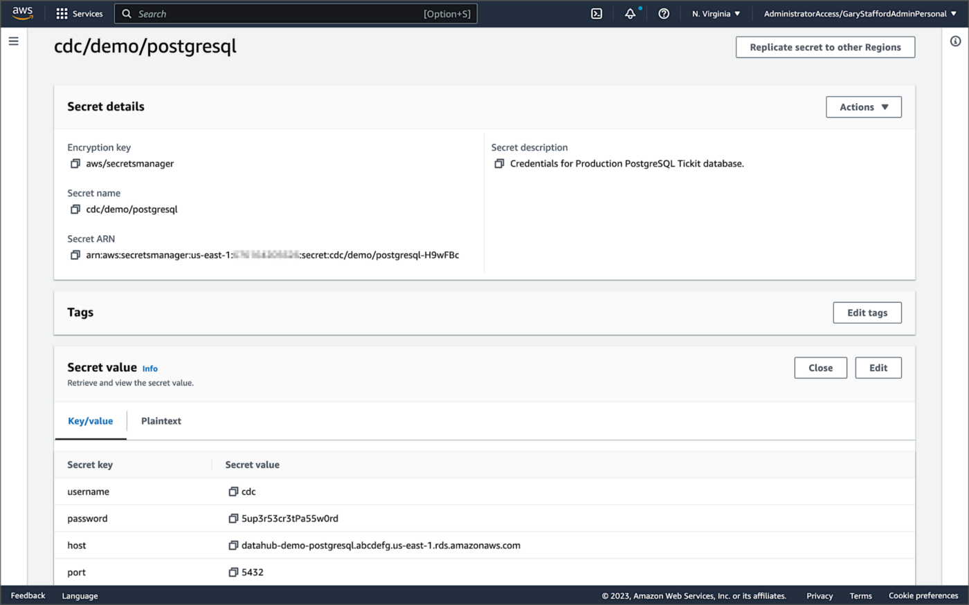
For self-managed Kafka Connect, I prefer Jeremy Custenborder’s kafka-config-provider-aws plugin. This plugin provides integration with AWS Secrets Manager. A complete list of Jeremy’s providers can be found on GitHub. Below is a snippet of the Secrets Manager configuration from the connect-distributed.properties files, which is read by Apache Kafka Connect at startup.
https://garystafford.medium.com/media/db6ff589c946fcd014546c56d0255fe5
Apache Avro
The message in the Kafka topic and corresponding objects in Amazon S3 will be stored in Apache Avro format by the CDC process. The Apache Avro documentation states, “Apache Avro is the leading serialization format for record data, and the first choice for streaming data pipelines.” Avro provides rich data structures and a compact, fast, binary data format.
Again, according to the Apache Avro documentation, “Avro relies on schemas. When Avro data is read, the schema used when writing it is always present. This permits each datum to be written with no per-value overheads, making serialization both fast and small. This also facilitates use with dynamic, scripting languages, since data, together with its schema, is fully self-describing.” When Avro data is stored in a file, its schema can be stored with it so any program may process files later.
Alternatively, the schema can be stored separately in a schema registry. According to Apicurio Registry, “in the messaging and event streaming world, data that are published to topics and queues often must be serialized or validated using a Schema (e.g. Apache Avro, JSON Schema, or Google protocol buffers). Schemas can be packaged in each application, but it is often a better architectural pattern to instead register them in an external system [schema registry] and then referenced from each application.”
Schema Registry
Several leading open-source and commercial schema registries exist, including Confluent Schema Registry, AWS Glue Schema Registry, and Red Hat’s open-source Apicurio Registry. In this post, we use a self-managed version of Apicurio Registry running on Amazon EKS. You can relatively easily substitute AWS Glue Schema Registry if you prefer a fully-managed AWS service.
Apicurio Registry
According to the documentation, Apicurio Registry supports adding, removing, and updating OpenAPI, AsyncAPI, GraphQL, Apache Avro, Google protocol buffers, JSON Schema, Kafka Connect schema, WSDL, and XML Schema (XSD) artifact types. Furthermore, content evolution can be controlled by enabling content rules, including validity and compatibility. Lastly, the registry can be configured to store data in various backend storage systems depending on the use case, including Kafka (e.g., Amazon MSK), PostgreSQL (e.g., Amazon RDS), and Infinispan (embedded).
Data Lake Table Formats
Three leading open-source, transactional data lake storage frameworks enable building data lake and data lakehouse architectures: Apache Iceberg, Linux Foundation Delta Lake, and Apache Hudi. They offer comparable features, such as ACID-compliant transactional guarantees, time travel, rollback, and schema evolution. Using any of these three data lake table formats will allow us to store and perform analytics on the latest version of the data in the data lake originating from the three Amazon RDS databases.
Apache Hudi
According to the Apache Hudi documentation, “Apache Hudi is a transactional data lake platform that brings database and data warehouse capabilities to the data lake.” The specifics of how the data is laid out as files in your data lake depends on the Hudi table type you choose, either Copy on Write (CoW) or Merge On Read (MoR).
Like Apache Iceberg and Delta Lake, Apache Hudi is partially supported by AWS’s Analytics services, including AWS Glue, Amazon EMR, Amazon Athena, Amazon Redshift Spectrum, and AWS Lake Formation. In general, CoW has broader support on AWS than MoR. It is important to understand the limitations of Apache Hudi with each AWS analytics service before choosing a table format.
If you are looking for a fully-managed Cloud data lake service built on Hudi, I recommend Onehouse. Born from the roots of Apache Hudi and founded by its original creator, Vinoth Chandar (PMC chair of the Apache Hudi project), the Onehouse product and its services leverage OSS Hudi to offer a data lake platform similar to what companies like Uber have built.
Hudi DeltaStreamer
Hudi also offers DeltaStreamer (aka HoodieDeltaStreamer) for streaming ingestion of CDC data. DeltaStreamer can be run once or continuously, using Apache Spark, similar to an Apache Spark Structured Streaming job, to capture changes to the raw CDC data and write that data to a different part of our data lake.
DeltaStreamer also works with Amazon S3 Event Notifications instead of running continuously. According to DeltaStreamer’s documentation, Amazon S3 object storage provides an event notification service to post notifications when certain events happen in your S3 bucket. AWS will put these events in Amazon Simple Queue Service (Amazon SQS). Apache Hudi provides an S3EventsSource that can read from Amazon SQS to trigger and process new or changed data as soon as it is available on Amazon S3.
Sample Data for the Data Lake
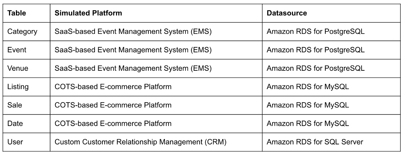
The data used in this post is from the TICKIT sample database. The TICKIT database represents the backend data store for a platform that brings buyers and sellers of tickets to entertainment events together. It was initially designed to demonstrate Amazon Redshift. The TICKIT database is a small database with approximately 425K rows of data across seven tables: Category, Event, Venue, User, Listing, Sale, and Date.
A data lake most often contains data from multiple sources, each with different storage formats, protocols, and connection methods. To simulate these data sources, I have separated the TICKIT database tables to represent three typical enterprise systems, including a commercial off-the-shelf (COTS) E-commerce platform, a custom Customer Relationship Management (CRM) platform, and a SaaS-based Event Management System (EMS). Each simulated system uses a different Amazon RDS database engine, including MySQL, PostgreSQL, and SQL Server.
Enabling CDC for Amazon RDS
To use Debezium for CDC with Amazon RDS databases, minor changes to the default database configuration for each database engine are required.
CDC for PostgreSQL
Debezium has detailed instructions regarding configuring CDC for Amazon RDS for PostgreSQL. Database parameters specify how the database is configured. According to the Debezium documentation, for PostgreSQL, set the instance parameter rds.logical_replication to 1 and verify that the wal_level parameter is set to logical. It is automatically changed when the rds.logical_replication parameter is set to 1. This parameter is adjusted using an Amazon RDS custom parameter group. According to the AWS documentation, “with Amazon RDS, you manage database configuration by associating your DB instances and Multi-AZ DB clusters with parameter groups. Amazon RDS defines parameter groups with default settings. You can also define your own parameter groups with customized settings.”

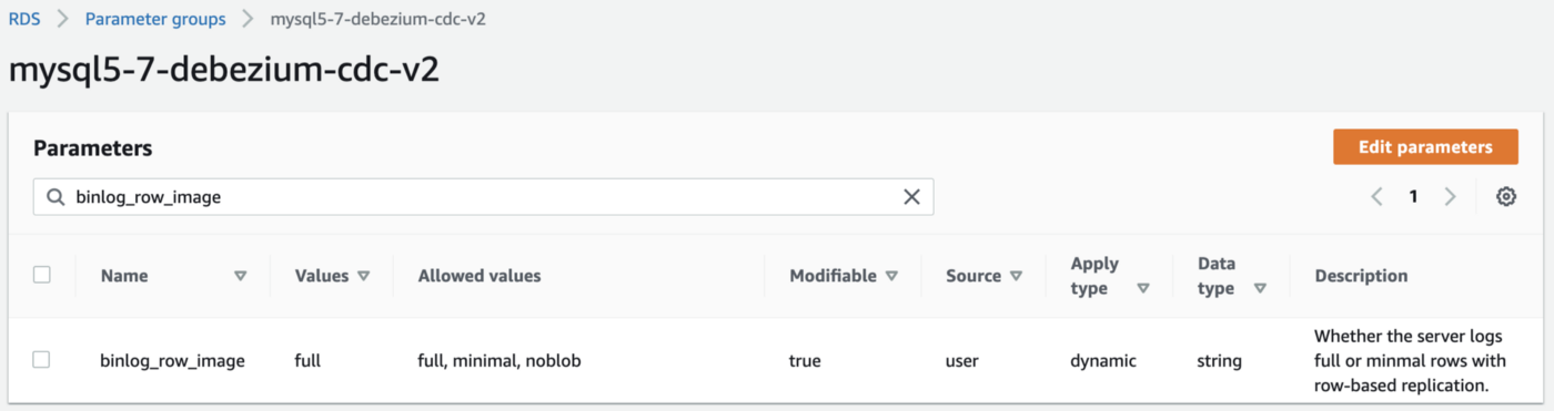
CDC for MySQL
Similarly, Debezium has detailed instructions regarding configuring CDC for MySQL. Like PostgreSQL, MySQL requires a custom DB parameter group.


CDC for SQL Server
Lastly, Debezium has detailed instructions for configuring CDC with Microsoft SQL Server. Enabling CDC requires enabling CDC on the SQL Server database and table(s) and creating a new filegroup and associated file. Debezium recommends locating change tables in a different filegroup than you use for source tables. CDC is only supported with Microsoft SQL Server Standard Edition and higher; Express and Web Editions are not supported.
Kafka Connect Source Connectors
There is a Kafka Connect source connector for each of the three Amazon RDS databases, all of which use Debezium. CDC is performed, moving changes from the three databases into separate Kafka topics in Apache Avro format using the source connectors. The connector configuration is nearly identical whether you are using Amazon MSK Connect or a self-managed version of Kafka Connect.
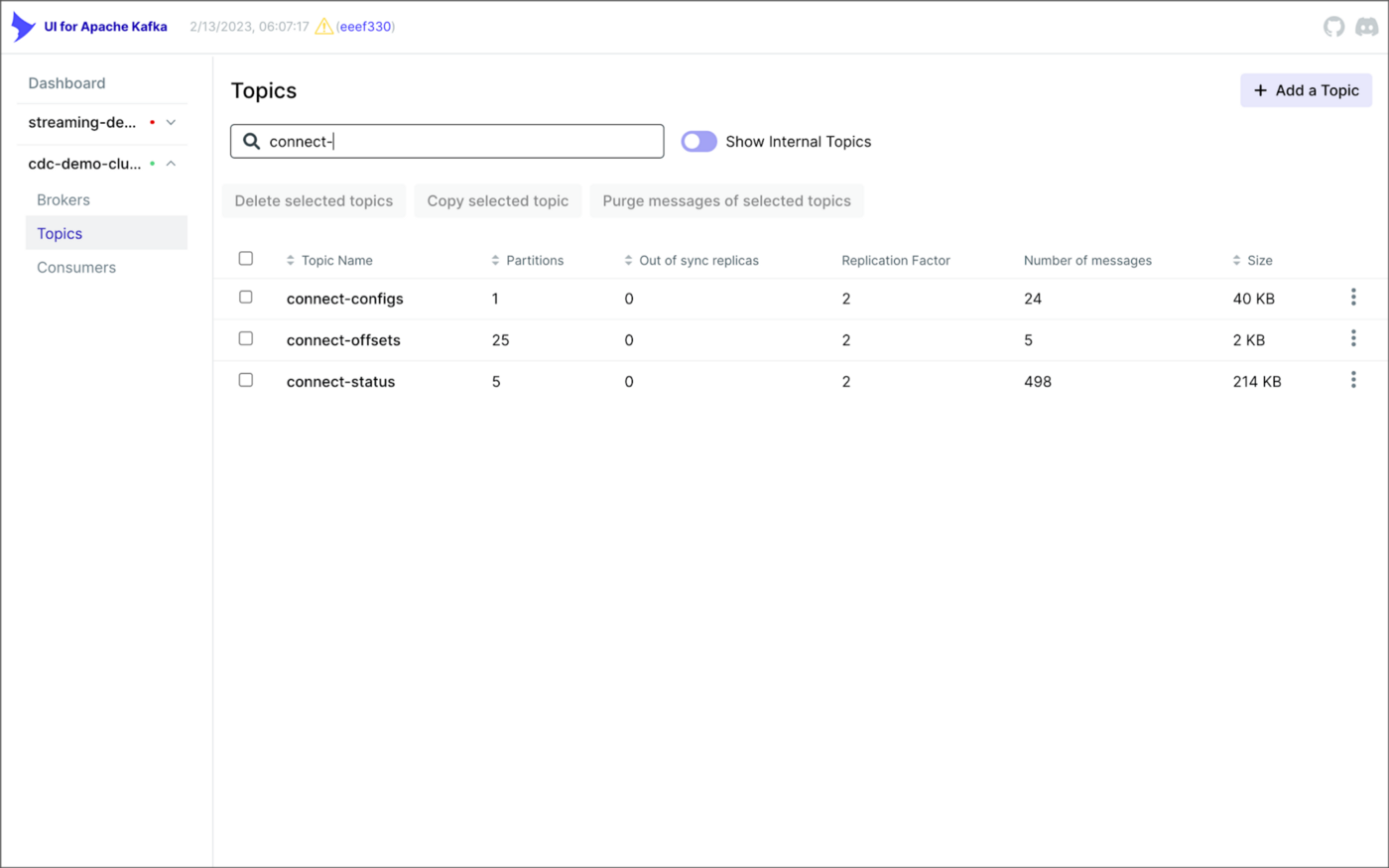
As shown above, I am using the UI for Apache Kafka by Provectus, self-managed on Amazon EKS, in this post.
PostgreSQL Source Connector
The source_connector_postgres_kafka_avro_tickit source connector captures all changes to the three tables in the Amazon RDS for PostgreSQL ticket database’s ems schema: category, event, and venue. These changes are written to three corresponding Kafka topics as Avro-format messages: tickit.ems.category, tickit.ems.event, and tickit.ems.venue. The messages are transformed by the connector using Debezium’s unwrap transform. Schemas for the messages are written to Apicurio Registry.
MySQL Source Connector
The source_connector_mysql_kafka_avro_tickit source connector captures all changes to the three tables in the Amazon RDS for PostgreSQL ecomm database: date, listing, and sale. These changes are written to three corresponding Kafka topics as Avro-format messages: tickit.ecomm.date, tickit.ecomm.listing, and tickit.ecomm.sale.
SQL Server Source Connector
Lastly, the source_connector_mssql_kafka_avro_tickit source connector captures all changes to the single user table in the Amazon RDS for SQL Server ticket database’s crm schema. These changes are written to a corresponding Kafka topic as Avro-format messages: tickit.crm.user.
If using a self-managed version of Kafka Connect, we can deploy, manage, and monitor the source and sink connectors using Kafka Connect’s RESTful API (Connect API).

Once the three source connectors are running, we should see seven new Kafka topics corresponding to the seven TICKIT database tables from the three Amazon RDS database sources. There will be approximately 425K messages consuming 147 MB of space in Avro’s binary format.
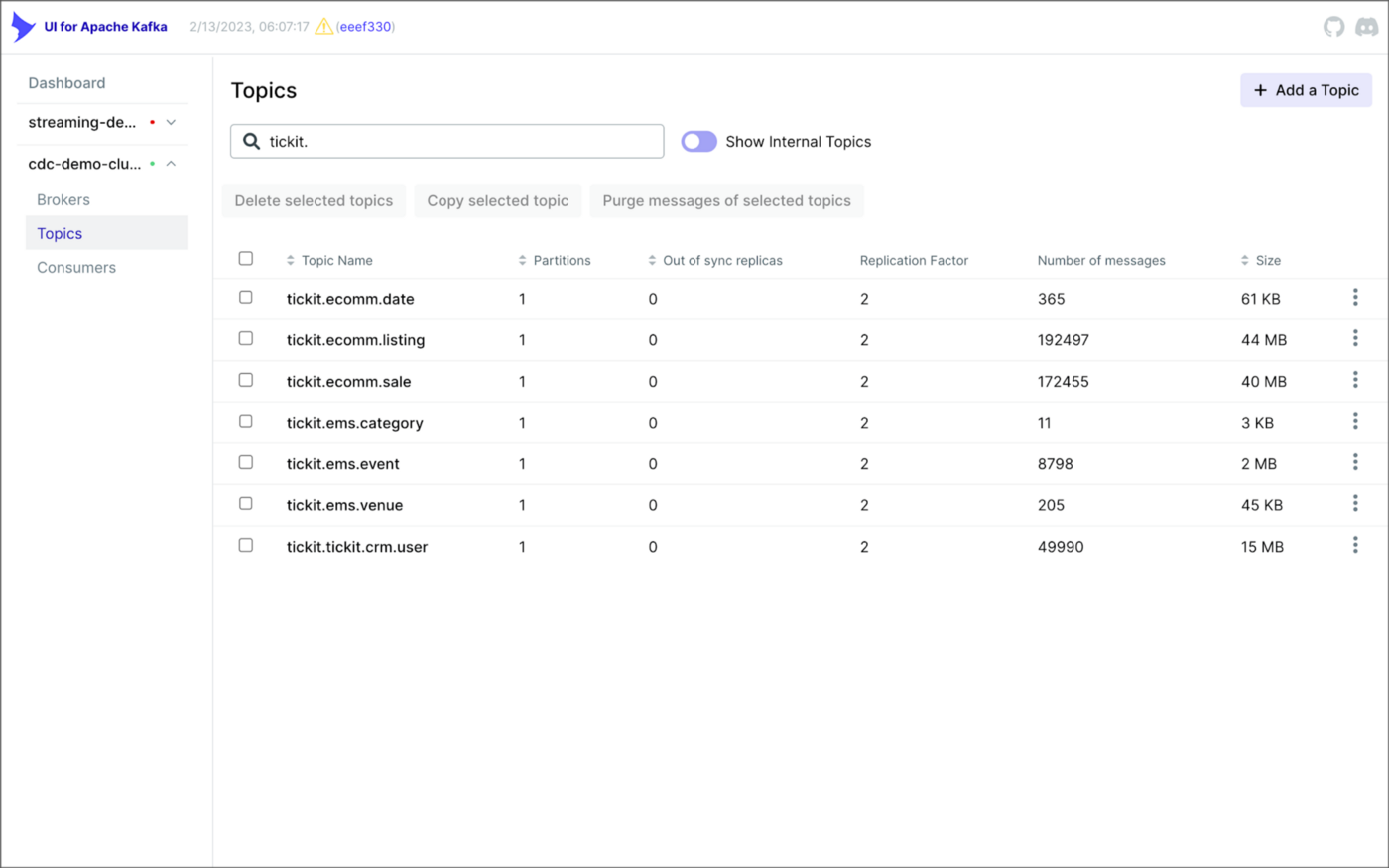
Avro’s binary format and the use of a separate schema ensure the messages consume minimal Kafka storage space. For example, the average message Value (payload) size in the tickit.ecomm.sale topic is a minuscule 98 Bytes. Resource management is critical when you are dealing with hundreds of millions or often billions of daily Kafka messages as a result of the CDC process.

From within the Apicurio Registry UI, we should now see Value schema artifacts for each of the seven Kafka topics.
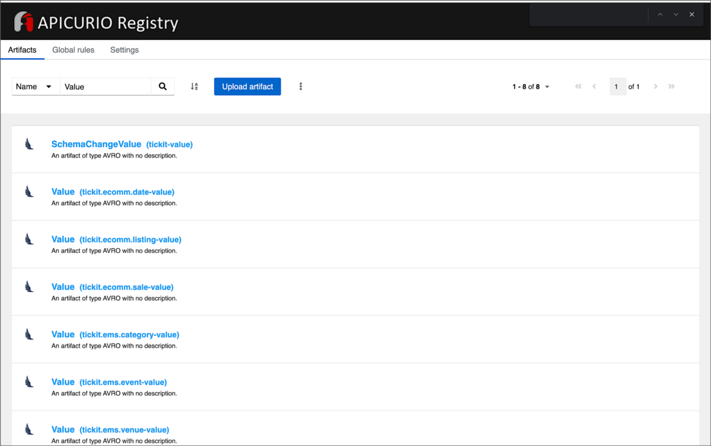
Also from within the Apicurio Registry UI, we can examine details of individual Value schema artifacts.

Kafka Connect Sink Connector
In addition to the three source connectors, there is a single Kafka Connect sink connector, sink_connector_kafka_s3_avro_tickit. The sink connector copies messages from the seven Kafka topics, all prefixed with tickit, to the Bronze area of our Amazon S3-based data lake.

The connector uses Confluent’s S3 Sink Connector (S3SinkConnector). Like Kafka, the connector writes all changes to Amazon S3 in Apache Avro format, with the schemas already stored in Apicurio Registry.
Once the sink connector and the three source connectors are running with Kafka Connect, we should see a series of seven subdirectories within the Bronze area of the data lake.

Confluent offers a choice of data partitioning strategies. The sink connector we have deployed uses the Daily Partitioner. According to the documentation, the io.confluent.connect.storage.partitioner.DailyPartitioner is equivalent to the TimeBasedPartitioner with path.format='year'=YYYY/'month'=MM/'day'=dd and partition.duration.ms=86400000 (one day for one S3 object in each daily directory). Below is an example of Avro files (S3 objects) containing changes to the sale table. The objects are partitioned by the year, month, and day they were written to the S3 bucket.

Message Transformation
Previously, while discussing the Kafka Connect source connectors, I mentioned that the connector transforms the messages using the unwrap transform. By default, the changes picked up by Debezium during the CDC process contain several additional Debezium-related fields of data. An example of an untransformed message generated by Debezium from the PostgreSQL sale table is shown below.
When the PostgreSQL connector first connects to a particular PostgreSQL database, it starts by performing a consistent snapshot of each database schema. All existing records are captured. Unlike an UPDATE ("op" : "u") or a DELETE ("op" : "d"), these initial snapshot messages, like the one shown below, represent a READ operation ("op" : "r"). As a result, there is no before data only after.
According to Debezium’s documentation, “Debezium provides a single message transformation [SMT] that crosses the bridge between the complex and simple formats, the UnwrapFromEnvelope SMT.” Below, we see the results of Debezium’s unwrap transform of the same message. The unwrap transform flattens the nested JSON structure of the original message, adds the __deleted field, and includes fields based on the list included in the source connector’s configuration. These fields are prefixed with a double underscore (e.g., __table).
In the next section, we examine Apache Hudi will manage the data lake. An example of the same message, managed with Hudi, is shown below. Note the five additional Hudi data fields, prefixed with _hoodie_.
Apache Hudi
With database changes flowing into the Bronze area of our data lake, we are ready to use Apache Hudi to provide data lake capabilities such as ACID transactional guarantees, time travel, rollback, and schema evolution. Using Hudi allows us to store and perform analytics on a specific time-bound version of the data in the data lake. Without Hudi, a query for a single row of data could return multiple results, such as an initial CREATE record, multiple UPDATE records, and a DELETE record.
DeltaStreamer
Using Hudi’s DeltaStreamer, we will continuously stream changes from the Bronze area of the data lake to a Silver area, which Hudi manages. We will run DeltaStreamer continuously, similar to an Apache Spark Structured Streaming job, using Apache Spark on Amazon EMR. Running DeltaStreamer requires using a spark-submit command that references a series of configuration files. There is a common base set of configuration items and a group of configuration items specific to each database table. Below, we see the base configuration, base.properties.
The base configuration is referenced by each of the table-specific configuration files. For example, below, we see the tickit.ecomm.sale.properties configuration file for DeltaStreamer.
To run DeltaStreamer, you can submit an EMR Step or use EMR’s master node to run a spark-submit command on the cluster. Below, we see an example of the DeltaStreamer spark-submit command using the Merge on Read (MoR) Hudi table type.
Next, we see the same example of the DeltaStreamer spark-submit command using the Copy on Write (CoW) Hudi table type.
For this post’s demonstration, we will run a single-table DeltaStreamer Spark job, with one process for each table using CoW. Alternately, Hudi offers HoodieMultiTableDeltaStreamer, a wrapper on top of HoodieDeltaStreamer, which enables the ingestion of multiple tables at a single time into Hudi datasets. Currently, HoodieMultiTableDeltaStreamer only supports sequential processing of tables to be ingested and COPY_ON_WRITE storage type.
Below, we see an example of three DeltaStreamer Spark jobs running continuously for the date, listing, and sale tables.

Once DeltaStreamer is up and running, we should see a series of subdirectories within the Silver area of the data lake, all managed by Apache Hudi.
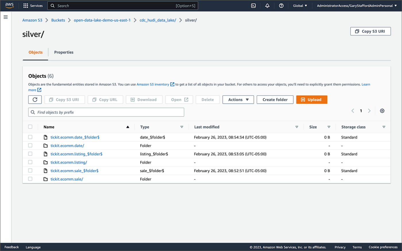
Within each subdirectory, partitioned by the table name, is a series of Apache Parquet files, along with other Apache Hudi-specific files. The specific folder structure and files depend on MoR or Cow.

AWS Glue Data Catalog
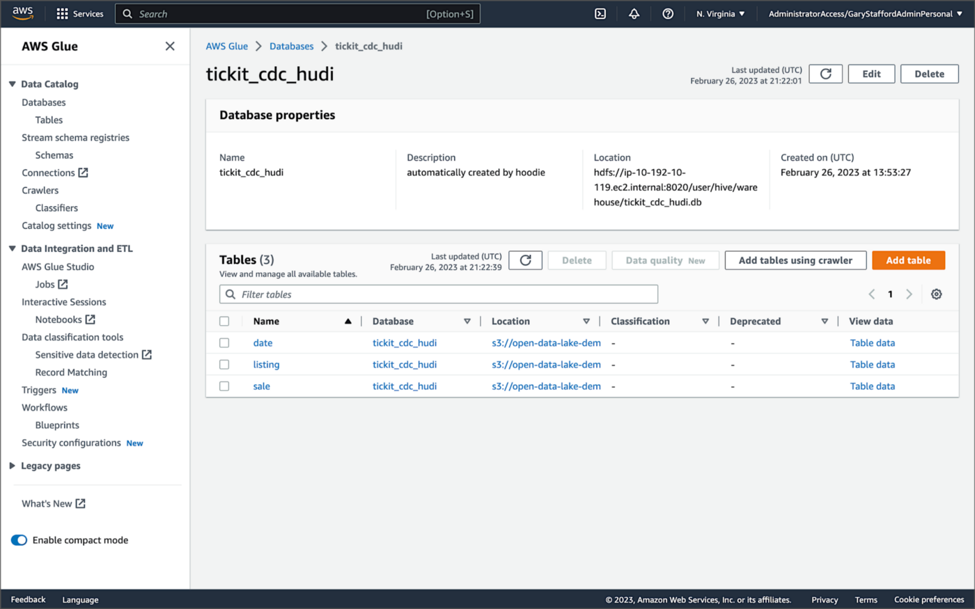
For this post, we are using an AWS Glue Data Catalog, an Apache Hive-compatible metastore, to persist technical metadata stored in the Silver area of the data lake, managed by Apache Hudi. The AWS Glue Data Catalog database, tickit_cdc_hudi, will be automatically created the first time DeltaStreamer runs.
Using DeltaStreamer with the table type of MERGE_ON_READ, there would be two tables in the AWS Glue Data Catalog database for each original table. According to Amazon’s EMR documentation, “Merge on Read (MoR) — Data is stored using a combination of columnar (Parquet) and row-based (Avro) formats. Updates are logged to row-based delta files and are compacted as needed to create new versions of the columnar files.” Hudi creates two tables in the Hive metastore for MoR, a table with the name that you specified, which is a read-optimized view (appended with _ro), and a table with the same name appended with _rt, which is a real-time view. You can query both tables.
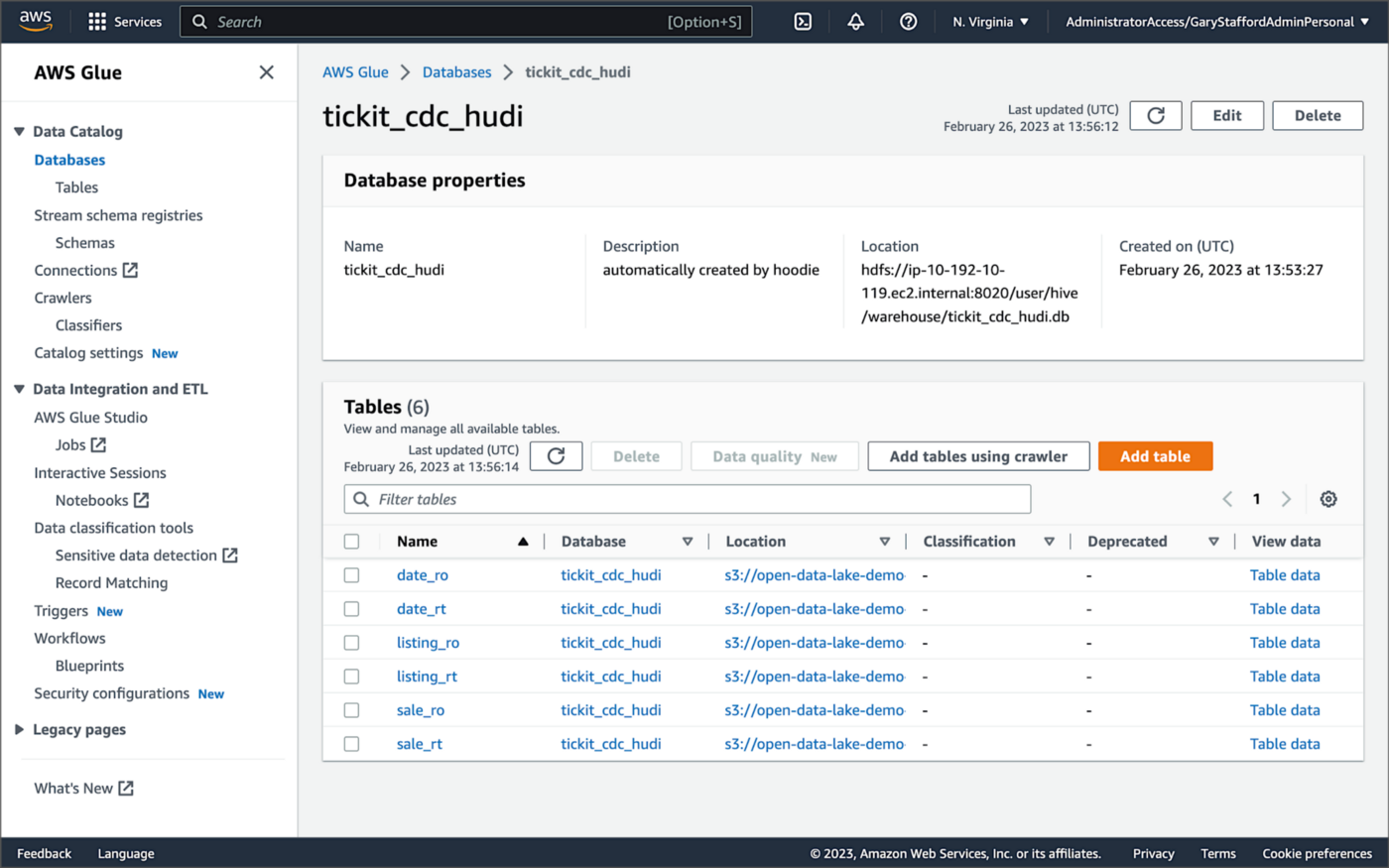
According to Amazon’s EMR documentation, “Copy on Write (CoW) — Data is stored in a columnar format (Parquet), and each update creates a new version of files during a write. CoW is the default storage type.” Using COPY_ON_WRITE with DeltaStreamer, there is only a single Hudi table in the AWS Glue Data Catalog database for each corresponding database table.
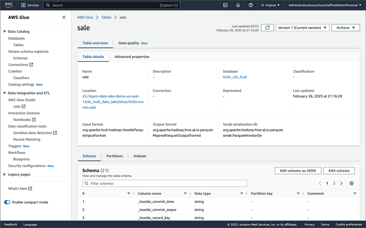
Examining an individual table in the AWS Glue Data Catalog database, we can see details like the table schema, location of underlying data in S3, input/output formats, Serde serialization library, and table partitions.
Database Changes and Data Lake
We are using Kafka Connect, Apache Hudi, and Hudi’s DeltaStreamer to maintain data parity between our databases and the data lake. Let’s look at an example of how a simple data change is propagated from a database to Kafka, then to the Bronze area of the data lake, and finally to the Hudi-managed Silver area of the data lake, written using the CoW table format.
First, we will make a simple update to a single record in the MySQL database’s sale table with the salesid = 200.
Almost immediately, we can see the change picked up by the Kafka Connect Debezium MySQL source connector.

Almost immediately, in the Bronze area of the data lake, we can see we have a new Avro-formatted file (S3 object) containing the updated record in the partitioned sale subdirectory.

If we examine the new object in the Bronze area of the data lake, we will see a row representing the updated record with the salesid = 200. Note how the operation is now an UPDATE versus a READ ("op" : "u").
Next, in the corresponding Silver area of the data lake, managed by Hudi, we should also see a new Parquet file that contains a record of the change. In this example, the file was written approximately 26 seconds after the original change to the database. This is the end-to-end time from database change to when the updated data is queryable in the data lake.
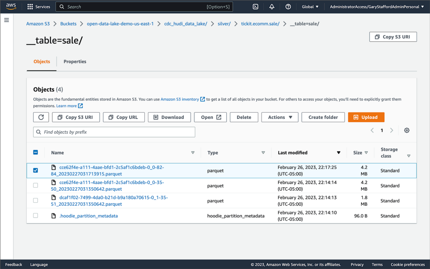
Similarly, if we examine the new object in the Silver area of the data lake, we will see a row representing the updated record with the salesid = 200. The record was committed approximately 15 seconds after the original database change.
Querying Hudi Tables with Amazon EMR
Using an EMR Notebook, we can query the updated database record stored in Amazon S3 using Hudi’s CoW table format. First, running a simple Spark SQL query for the record with salesid = 200, returns the latest record, reflecting the changes as indicated by the UPDATE operation value (u) and the _hoodie_commit_time = 2023-02-27 03:17:13.915 UTC.

Hudi Time Travel Query
We can also run a Hudi Time Travel Query, with an as.of.instance set to some arbitrary point in the future. Again, the latest record is returned, reflecting the changes as indicated by the UPDATE operation value (u) and the _hoodie_commit_time = 2023-02-27 03:17:13.915 UTC.

We can run the same Hudi Time Travel Query with an as.of.instance set to on or after the original records were written by DeltaStreamer (_hoodie_commit_time = 2023-02-27 03:13:50.642), but some arbitrary time before the updated record was written (_hoodie_commit_time = 2023-02-27 03:17:13.915). This time, the original record is returned as indicated by the READ operation value (r) and the _hoodie_commit_time = 2023-02-27 03:13:50.642. This is one of the strengths of Apache Hudi, the ability to query data in the present or at any point in the past.

Hudi Point in Time Query
We can also run a Hudi Point in Time Query, with a time range set from the beginning of time until some arbitrary point in the future. Again, the latest record is returned, reflecting the changes as indicated by the UPDATE operation value (u) and the _hoodie_commit_time = 2023-02-27 03:17:13.915.

We can run the same Hudi Point in Time Query but change the time range to two arbitrary time values, both before the updated record was written (_hoodie_commit_time = 2023-02-26 22:39:07.203). This time, the original record is returned as indicated by the READ operation value (r) and the _hoodie_commit_time of 2023-02-27 03:13:50.642. Again, this is one of the strengths of Apache Hudi, the ability to query data in the present or at any point in the past.

Querying Hudi Tables with Amazon Athena
We can also use Amazon Athena and run a SQL query against the AWS Glue Data Catalog database’s sale table to view the updated database record stored in Amazon S3 using Hudi’s CoW table format. The operation (op) column’s value now indicates an UPDATE (u).

How are Deletes Handled?
In this post’s architecture, deleted database records are signified with an operation ("op") field value of "d" for a DELETE and a __deleted field value of true.
https://itnext.io/media/f7c4ad62dcd45543fdf63834814a5aab
Back to our previous Jupyter notebook example, when rerunning the Spark SQL query, the latest record is returned, reflecting the changes as indicated by the DELETE operation value (d) and the _hoodie_commit_time = 2023-02-27 03:52:13.689.

Alternatively, we could use an additional Spark SQL filter statement to prevent deleted records from being returned (e.g., df.__op != "d").

Since we only did what is referred to as a soft delete in Hudi terminology, we can run a time travel query with an as.of.instance set to some arbitrary time before the deleted record was written (_hoodie_commit_time = 2023-02-27 03:52:13.689). This time, the original record is returned as indicated by the READ operation value (r) and the _hoodie_commit_time = 2023-02-27 03:13:50.642. We could also use a later as.of.instance to return the version of the record reflecting the the UPDATE operation value (u). This also applies to other query types such as point-in-time queries.

Conclusion
In this post, we learned how to build a near real-time transactional data lake on AWS using one possible architecture. The data lake was built using a combination of open source software (OSS) and fully-managed AWS services. Red Hat’s Debezium, Apache Kafka, and Kafka Connect were used for change data capture (CDC). In addition, Apache Spark, Apache Hudi, and Hudi’s DeltaStreamer were used to manage the data lake. To complete our architecture, we used several fully-managed AWS services, including Amazon RDS, Amazon MKS, Amazon EKS, AWS Glue, and Amazon EMR.
This blog represents my own viewpoints and not of my employer, Amazon Web Services (AWS). All product names, logos, and brands are the property of their respective owners.
Utilizing In-memory Data Caching to Enhance the Performance of Data Lake-based Applications
Posted by Gary A. Stafford in Analytics, AWS, Big Data, Cloud, Java Development, Software Development, SQL on July 12, 2022
Significantly improve the performance and reduce the cost of data lake-based analytics applications using Amazon ElastiCache for Redis
Introduction
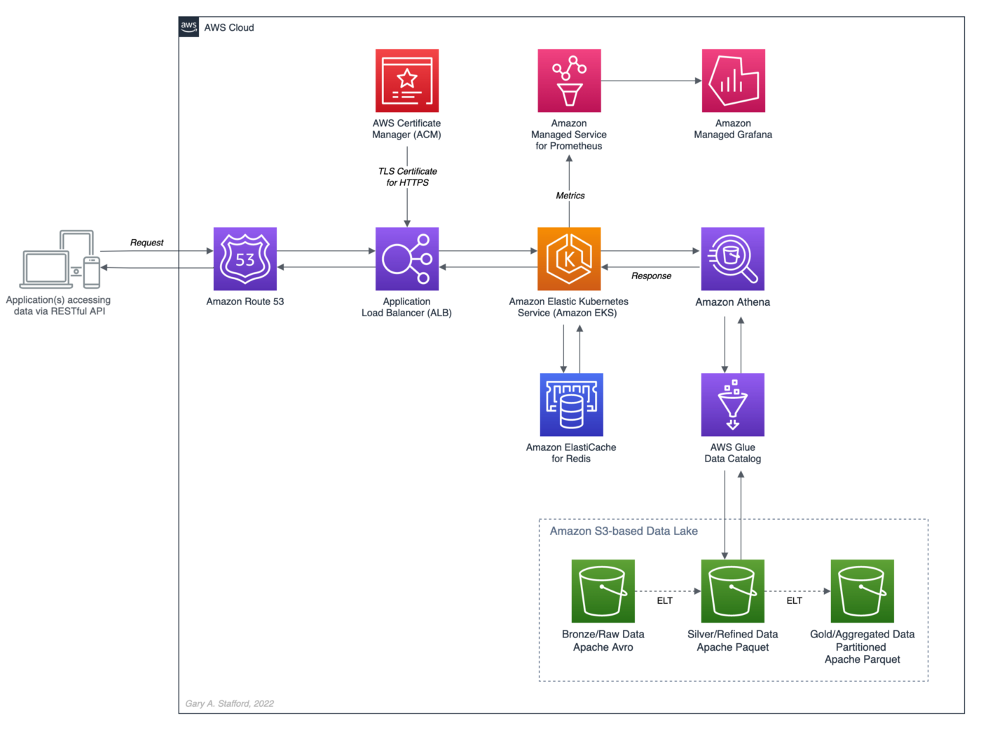
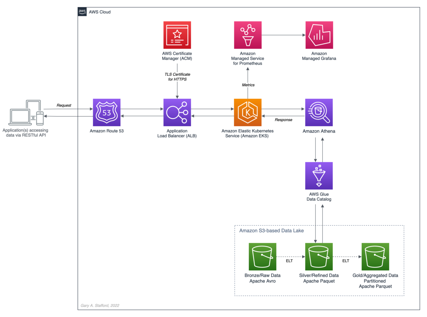
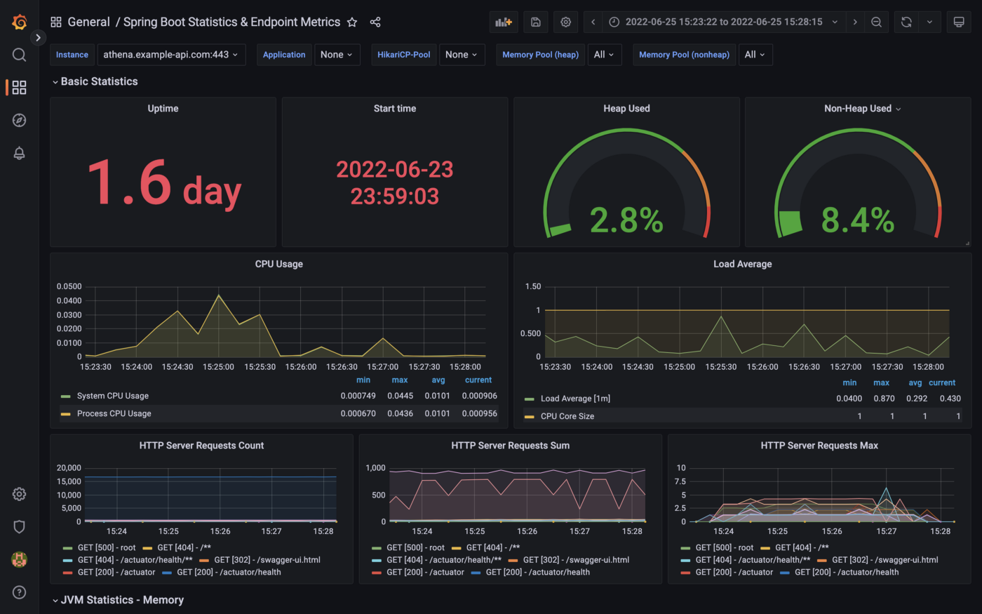
The recent post, Developing Spring Boot Applications for Querying Data Lakes on AWS using Amazon Athena, demonstrated how to develop a Cloud-native analytics application using Spring Boot. The application queried data in an Amazon S3-based data lake via an AWS Glue Data Catalog utilizing the Amazon Athena API.
Securely exposing data in a data lake using RESTful APIs can fulfill many data-consumer needs. However, access to that data can be significantly slower than access from a database or data warehouse. For example, in the previous post, we imported the OpenAPI v3 specification from the Spring Boot service into Postman. The API specification contained approximately 17 endpoints.
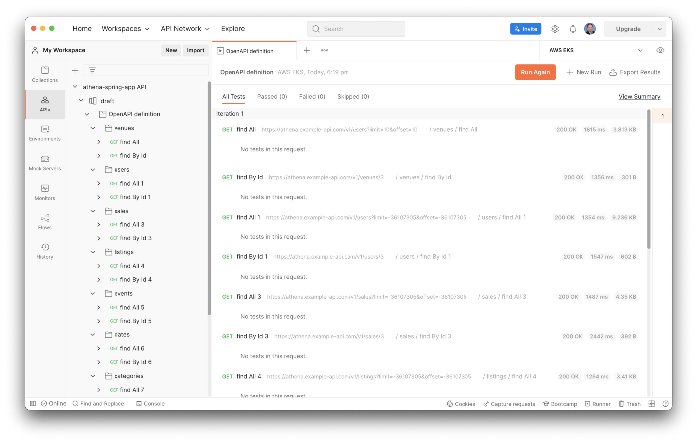
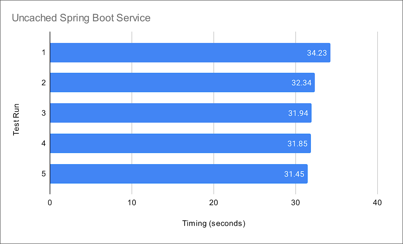
From my local development laptop, the Postman API test run times for all service endpoints took an average of 32.4 seconds. The Spring Boot service was running three Kubernetes pod replicas on Amazon EKS in the AWS US East (N. Virginia) Region.
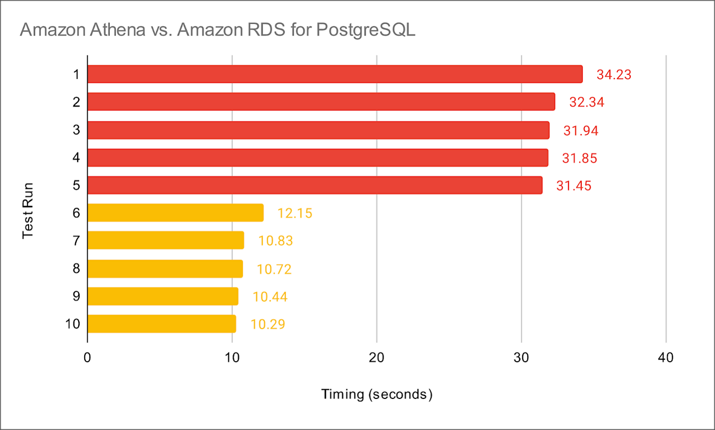
Compare the data lake query result times to equivalent queries made against a minimally-sized Amazon RDS for PostgreSQL database instance containing the same data. The average run times for all PostgreSQL queries averaged 10.8 seconds from a similar Spring Boot service. Although not a precise benchmark, we can clearly see that access to the data in the Amazon S3-based data lake is substantially slower, approximately 3x slower, than that of the PostgreSQL database. Tuning the database would easily create an even greater disparity.
Caching for Data Lakes
According to AWS, the speed and throughput of a database can be the most impactful factor for overall application performance. Consequently, in-memory data caching can be one of the most effective strategies to improve overall application performance and reduce database costs. This same caching strategy can be applied to analytics applications built atop data lakes, as this post will demonstrate.
In-memory Caching
According to Hazelcast, memory caching (aka in-memory caching), often simply referred to as caching, is a technique in which computer applications temporarily store data in a computer’s main memory (e.g., RAM) to enable fast retrievals of that data. The RAM used for the temporary storage is known as the cache. As an application tries to read data, typically from a data storage system like a database, it checks to see if the desired record already exists in the cache. If it does, the application will read the data from the cache, thus eliminating the slower access to the database. If the desired record is not in the cache, then the application reads the record from the source. When it retrieves that data, it writes it to the cache so that when the application needs that same data in the future, it can quickly retrieve it from the cache.
Further, according to Hazelcast, as an application tries to read data, typically from a data storage system like a database, it checks to see if the desired record already exists in the cache. If it does, the application will read the data from the cache, thus eliminating the slower access to the database. If the desired record is not in the cache, then the application reads the record from the source. When it retrieves that data, it writes it to the cache so that when the application needs that same data in the future, it can quickly retrieve it from the cache.
Redis In-memory Data Store
According to their website, Redis is the open-source, in-memory data store used by millions of developers as a database, cache, streaming engine, and message broker. Redis provides data structures such as strings, hashes, lists, sets, sorted sets with range queries, bitmaps, hyperloglogs, geospatial indexes, and streams. In addition, Redis has built-in replication, Lua scripting, LRU eviction, transactions, and different levels of on-disk persistence and provides high availability via Redis Sentinel and automatic partitioning with Redis Cluster.
Amazon ElastiCache for Redis
According to AWS, Amazon ElastiCache for Redis, the fully-managed version of Redis, according to AWS, is a blazing fast in-memory data store that provides sub-millisecond latency to power internet-scale real-time applications. Redis applications can work seamlessly with ElastiCache for Redis without any code changes. ElastiCache for Redis combines the speed, simplicity, and versatility of open-source Redis with manageability, security, and scalability from AWS. As a result, Redis is an excellent choice for implementing a highly available in-memory cache to decrease data access latency, increase throughput, and ease the load on relational and NoSQL databases.
ElastiCache Performance Results
In the following post, we will add in-memory caching to the Spring Boot service introduced in the previous post. In preliminary tests with Amazon ElastiCache for Redis, the Spring Boot service delivered a 34x improvement in average response times. For example, test runs with the best-case scenario of a Redis cache hit ratio of 100% averaged 0.95 seconds compared to 32.4 seconds without Redis.

Source Code
All the source code and Docker and Kubernetes resources are open-source and available on GitHub.
git clone --depth 1 -b redis \
    https://github.com/garystafford/athena-spring-app.git
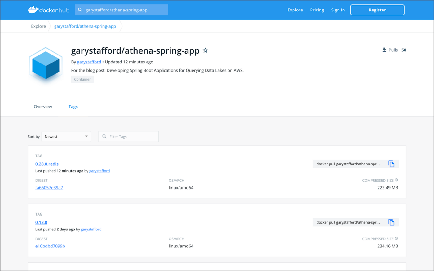
In addition, a Docker image for the Redis-base Spring Boot service is available on Docker Hub. For this post, use the latest tag with the .redis suffix.
Code Changes
The following code changes are required to the Spring Boot service to implement Spring Boot Cache with Redis.
Gradle Build
The gradle.build file now implements two additional dependencies, Spring Boot’s spring-boot-starter-cache and spring-boot-starter-data-redis (lines 45–46).
Application Properties
The application properties file, application.yml, has been modified for both the dev and prod Spring Profiles. The dev Spring Profile expects Redis to be running on localhost. Correspondingly, the project’s docker-compose.yml file now includes a Redis container for local development. The time-to-live (TTL) for all Redis caches is arbitrarily set to one minute for dev and five minutes for prod. To increase application performance and reduce the cost of querying the data lake using Athena, increase Redis’s TTL. Note that increasing the TTL will reduce data freshness.
Athena Application Class
The AthenaApplication class declaration is now decorated with Spring Framework’s EnableCaching annotation (line 22). Additionally, two new Beans have been added (lines 58–68). Spring Redis provides an implementation for the Spring cache abstraction through the org.springframework.data.redis.cache package. The RedisCacheManager cache manager creates caches by default upon the first write. The RedisCacheConfiguration cache configuration helps to customize RedisCache behavior such as caching null values, cache key prefixes, and binary serialization.
POJO Data Model Classes
Spring Boot Redis caching uses Java serialization and deserialization. Therefore, all the POJO data model classes must implement Serializable (line 14).
Service Classes
Each public method in the Service classes is now decorated with Spring Framework’s Cachable annotation (lines 42 and 66). For example, the findById(int id) method in the CategoryServiceImp class is annotated with @Cacheable(value = "categories", key = "#id"). The method’s key parameter uses Spring Expression Language (SpEL) expression for computing the key dynamically. Default is null, meaning all method parameters are considered as a key unless a custom keyGenerator has been configured. If no value is found in the Redis cache for the computed key, the target method will be invoked, and the returned value will be stored in the associated cache.
Controller Classes
There are no changes required to the Controller classes.
Amazon ElastiCache for Redis
Multiple options are available for creating an Amazon ElastiCache for Redis cluster, including cluster mode, multi-AZ option, auto-failover option, node type, number of replicas, number of shards, replicas per shard, Availability Zone placements, and encryption at rest and encryption in transit options. The results in this post are based on a minimally-configured Redis version 6.2.6 cluster, with one shard, two cache.r6g.large nodes, and cluster mode, multi-AZ option, and auto-failover all disabled. In addition, encryption at rest and encryption in transit were also disabled. This cluster configuration is sufficient for development and testing, but not Production.


Testing the Cache
To test Amazon ElastiCache for Redis, we will use Postman again with the imported OpenAPI v3 specification. With all data evicted from existing Redis caches, the first time the Postman tests run, they cause the service’s target methods to be invoked and the returned data stored in the associated caches.
To confirm this caching behavior, use the Redis CLI’s --scan option. To access the redis-cli, I deployed a single Redis pod to Amazon EKS. The first time the --scan command runs, we should get back an empty list of keys. After the first Postman test run, the same --scan command should return a list of cached keys.

Use the Redis CLI’s MONITOR option to further confirm data is being cached, as indicated by the set command.

After the initial caching of data, use the Redis CLI’s MONITOR option, again, to confirm the cache is being hit instead of calling the target methods, which would then invoke the Athena API. Rerunning the Postman tests, we should see get commands as opposed to set commands.

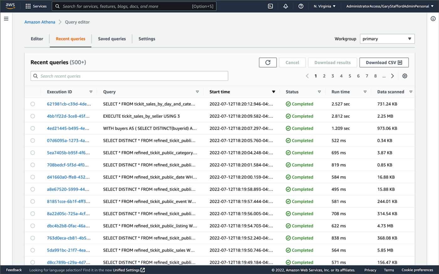
Lastly, to confirm the Spring Boot service is effectively using Redis to cache data, we can also check Amazon Athena’s Recent queries tab in the AWS Management Console. After repeated sequential test runs within the TTL window, we should only see one Athena query per endpoint.
Conclusion
In this brief follow-up to the recent post, Developing Spring Boot Applications for Querying Data Lakes on AWS using Amazon Athena, we saw how to substantially increase data lake application performance using Amazon ElastiCache for Redis. Although this caching technique is often associated with databases, it can also be effectively applied to data lake-based applications, as demonstrated in the post.
This blog represents my viewpoints and not of my employer, Amazon Web Services (AWS). All product names, logos, and brands are the property of their respective owners. All diagrams and illustrations are property of the author unless otherwise noted.
Developing Spring Boot Applications for Querying Data Lakes on AWS using Amazon Athena
Posted by Gary A. Stafford in Analytics, AWS, Big Data, Cloud, Java Development, Software Development on June 26, 2022
Learn how to develop Cloud-native, RESTful Java services that query data in an AWS-based data lake using Amazon Athena’s API
Introduction
AWS provides a collection of fully-managed services that makes building and managing secure data lakes faster and easier, including AWS Lake Formation, AWS Glue, and Amazon S3. Additional analytics services such as Amazon EMR, AWS Glue Studio, and Amazon Redshift allow Data Scientists and Analysts to run high-performance queries on large volumes of semi-structured and structured data quickly and economically.
What is not always as obvious is how teams develop internal and external customer-facing analytics applications built on top of data lakes. For example, imagine sellers on an eCommerce platform, the scenario used in this post, want to make better marketing decisions regarding their products by analyzing sales trends and buyer preferences. Further, suppose the data required for the analysis must be aggregated from multiple systems and data sources; the ideal use case for a data lake.
salesbyseller endpointIn this post, we will explore an example Java Spring Boot RESTful Web Service that allows end-users to query data stored in a data lake on AWS. The RESTful Web Service will access data stored as Apache Parquet in Amazon S3 through an AWS Glue Data Catalog using Amazon Athena. The service will use Spring Boot and the AWS SDK for Java to expose a secure, RESTful Application Programming Interface (API).
Amazon Athena is a serverless, interactive query service based on Presto, used to query data and analyze big data in Amazon S3 using standard SQL. Using Athena functionality exposed by the AWS SDK for Java and Athena API, the Spring Boot service will demonstrate how to access tables, views, prepared statements, and saved queries (aka named queries).

TL;DR
Do you want to explore the source code for this post’s Spring Boot service or deploy it to Kubernetes before reading the full article? All the source code, Docker, and Kubernetes resources are open-source and available on GitHub.
git clone --depth 1 -b main \
    https://github.com/garystafford/athena-spring-app.git
A Docker image for the Spring Boot service is also available on Docker Hub.

Data Lake Data Source
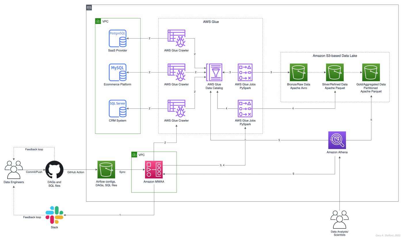
There are endless data sources to build a demonstration data lake on AWS. This post uses the TICKIT sample database provided by AWS and designed for Amazon Redshift, AWS’s cloud data warehousing service. The database consists of seven tables. Two previous posts and associated videos, Building a Data Lake on AWS with Apache Airflow and Building a Data Lake on AWS, detail the setup of the data lake used in this post using AWS Glue and optionally Apache Airflow with Amazon MWAA.
Those two posts use the data lake pattern of segmenting data as bronze (aka raw), silver (aka refined), and gold (aka aggregated), popularized by Databricks. The data lake simulates a typical scenario where data originates from multiple sources, including an e-commerce platform, a CRM system, and a SaaS provider must be aggregated and analyzed.
Spring Projects with IntelliJ IDE
Although not a requirement, I used JetBrains IntelliJ IDEA 2022 (Ultimate Edition) to develop and test the post’s Spring Boot service. Bootstrapping Spring projects with IntelliJ is easy. Developers can quickly create a Spring project using the Spring Initializr plugin bundled with the IntelliJ.

The Spring Initializr plugin’s new project creation wizard is based on start.spring.io. The plugin allows you to quickly select the Spring dependencies you want to incorporate into your project.

Visual Studio Code
There are also several Spring extensions for the popular Visual Studio Code IDE, including Microsoft’s Spring Initializr Java Support extension.

Gradle
This post uses Gradle instead of Maven to develop, test, build, package, and deploy the Spring service. Based on the packages selected in the new project setup shown above, the Spring Initializr plugin’s new project creation wizard creates a build.gradle file. Additional packages, such as Lombak, Micrometer, and Rest Assured, were added separately.
Amazon Corretto
The Spring boot service is developed for and compiled with the most recent version of Amazon Corretto 17. According to AWS, Amazon Corretto is a no-cost, multiplatform, production-ready distribution of the Open Java Development Kit (OpenJDK). Corretto comes with long-term support that includes performance enhancements and security fixes. Corretto is certified as compatible with the Java SE standard and is used internally at Amazon for many production services.
Source Code
Each API endpoint in the Spring Boot RESTful Web Service has a corresponding POJO data model class, service interface and service implementation class, and controller class. In addition, there are also common classes such as configuration, a client factory, and Athena-specific request/response methods. Lastly, there are additional class dependencies for views and prepared statements.

refined_tickit_public_category tableThe project’s source code is arranged in a logical hierarchy by package and class type.
Amazon Athena Access
There are three standard methods for accessing Amazon Athena with the AWS SDK for Java: 1) the AthenaClient service client, 2) the AthenaAsyncClient service client for accessing Athena asynchronously, and 3) using the JDBC driver with the AWS SDK. The AthenaClient and AthenaAsyncClient service clients are both parts of the software.amazon.awssdk.services.athena package. For simplicity, this post’s Spring Boot service uses the AthenaClient service client instead of Java’s asynchronously programming model. AWS supplies basic code samples as part of their documentation as a starting point for writing Athena applications using the SDK. The code samples also use the AthenaClient service client.
POJO-based Data Model Class
For each API endpoint in the Spring Boot RESTful Web Service, there is a corresponding Plain Old Java Object (POJO). According to Wikipedia, a POGO is an ordinary Java object, not bound by any particular restriction. The POJO class is similar to a JPA Entity, representing persistent data stored in a relational database. In this case, the POJO uses Lombok’s @Data annotation. According to the documentation, this annotation generates getters for all fields, a useful toString method, and hashCode and equals implementations that check all non-transient fields. It also generates setters for all non-final fields and a constructor.
Each POJO corresponds directly to a ‘silver’ table in the AWS Glue Data Catalog. For example, the Event POJO corresponds to the refined_tickit_public_event table in the tickit_demo Data Catalog database. The POJO defines the Spring Boot service’s data model for data read from the corresponding AWS Glue Data Catalog table.

The Glue Data Catalog table is the interface between the Athena query and the underlying data stored in Amazon S3 object storage. The Athena query targets the table, which returns the underlying data from S3.

Service Class
Retrieving data from the data lake via AWS Glue, using Athena, is handled by a service class. For each API endpoint in the Spring Boot RESTful Web Service, there is a corresponding Service Interface and implementation class. The service implementation class uses Spring Framework’s @Service annotation. According to the documentation, it indicates that an annotated class is a “Service,” initially defined by Domain-Driven Design (Evans, 2003) as “an operation offered as an interface that stands alone in the model, with no encapsulated state.” Most importantly for the Spring Boot service, this annotation serves as a specialization of @Component, allowing for implementation classes to be autodetected through classpath scanning.
Using Spring’s common constructor-based Dependency Injection (DI) method (aka constructor injection), the service auto-wires an instance of the AthenaClientFactory interface. Note that we are auto-wiring the service interface, not the service implementation, allowing us to wire in a different implementation if desired, such as for testing.
The service calls the AthenaClientFactoryclass’s createClient() method, which returns a connection to Amazon Athena using one of several available authentication methods. The authentication scheme will depend on where the service is deployed and how you want to securely connect to AWS. Some options include environment variables, local AWS profile, EC2 instance profile, or token from the web identity provider.
The service class transforms the payload returned by an instance of GetQueryResultsResponse into an ordered collection (also known as a sequence), List<E>, where E represents a POJO. For example, with the data lake’srefined_tickit_public_event table, the service returns a List<Event>. This pattern repeats itself for tables, views, prepared statements, and named queries. Column data types can be transformed and formatted on the fly, new columns added, and existing columns skipped.
For each endpoint defined in the Controller class, for example, get(), findAll(), and FindById(), there is a corresponding method in the Service class. Below, we see an example of the findAll() method in the SalesByCategoryServiceImp service class. This method corresponds to the identically named method in the SalesByCategoryController controller class. Each of these service methods follows a similar pattern of constructing a dynamic Athena SQL query based on input parameters, which is passed to Athena through the AthenaClient service client using an instance of GetQueryResultsRequest.
Controller Class
Lastly, there is a corresponding Controller class for each API endpoint in the Spring Boot RESTful Web Service. The controller class uses Spring Framework’s @RestController annotation. According to the documentation, this annotation is a convenience annotation that is itself annotated with @Controller and @ResponseBody. Types that carry this annotation are treated as controllers where @RequestMapping methods assume @ResponseBody semantics by default.
The controller class takes a dependency on the corresponding service class application component using constructor-based Dependency Injection (DI). Like the service example above, we are auto-wiring the service interface, not the service implementation.
The controller is responsible for serializing the ordered collection of POJOs into JSON and returning that JSON payload in the body of the HTTP response to the initial HTTP request.
Querying Views
In addition to querying AWS Glue Data Catalog tables (aka Athena tables), we also query views. According to the documentation, a view in Amazon Athena is a logical table, not a physical table. Therefore, the query that defines a view runs each time the view is referenced in a query.
For convenience, each time the Spring Boot service starts, the main AthenaApplication class calls the View.java class’s CreateView() method to check for the existence of the view, view_tickit_sales_by_day_and_category. If the view does not exist, it is created and becomes accessible to all application end-users. The view is queried through the service’s /salesbycategory endpoint.

This confirm-or-create pattern is repeated for the prepared statement in the main AthenaApplication class (detailed in the next section).
Below, we see the View class called by the service at startup.
Aside from the fact the /salesbycategory endpoint queries a view, everything else is identical to querying a table. This endpoint uses the same model-service-controller pattern.
Executing Prepared Statements
According to the documentation, you can use the Athena parameterized query feature to prepare statements for repeated execution of the same query with different query parameters. The prepared statement used by the service, tickit_sales_by_seller, accepts a single parameter, the ID of the seller (sellerid). The prepared statement is executed using the /salesbyseller endpoint. This scenario simulates an end-user of the analytics application who wants to retrieve enriched sales information about their sales.
The pattern of querying data is similar to tables and views, except instead of using the common SELECT...FROM...WHERE SQL query pattern, we use the EXECUTE...USING pattern.
For example, to execute the prepared statement for a seller with an ID of 3, we would use EXECUTE tickit_sales_by_seller USING 3;. We pass the seller’s ID of 3 as a path parameter similar to other endpoints exposed by the service: /v1/salesbyseller/3.

Again, aside from the fact the /salesbyseller endpoint executes a prepared statement and passes a parameter; everything else is identical to querying a table or a view, using the same model-service-controller pattern.
Working with Named Queries
In addition to tables, views, and prepared statements, Athena has the concept of saved queries, referred to as named queries in the Athena API and when using AWS CloudFormation. You can use the Athena console or API to save, edit, run, rename, and delete queries. The queries are persisted using a NamedQueryId, a unique identifier (UUID) of the query. You must reference the NamedQueryId when working with existing named queries.

There are multiple ways to use and reuse existing named queries programmatically. For this demonstration, I created the named query, buyer_likes_by_category, in advance and then stored the resulting NamedQueryId as an application property, injected at runtime or kubernetes deployment time through a local environment variable.
Alternately, you might iterate through a list of named queries to find one that matches the name at startup. However, this method would undoubtedly impact service performance, startup time, and cost. Lastly, you could use a method like NamedQuery() included in the unused NamedQuery class at startup, similar to the view and prepared statement. That named query’s unique NamedQueryId would be persisted as a system property, referencable by the service class. The downside is that you would create a duplicate of the named query each time you start the service. Therefore, this method is also not recommended.
Configuration
Two components responsible for persisting configuration for the Spring Boot service are the application.yml properties file and ConfigProperties class. The class uses Spring Framework’s @ConfigurationProperties annotation. According to the documentation, this annotation is used for externalized configuration. Add this to a class definition or a @Bean method in a @Configuration class if you want to bind and validate some external Properties (e.g., from a .properties or .yml file). Binding is performed by calling setters on the annotated class or, if @ConstructorBinding in use, by binding to the constructor parameters.
The @ConfigurationProperties annotation includes the prefix of athena. This value corresponds to the athena prefix in the the application.yml properties file. The fields in the ConfigProperties class are bound to the properties in the the application.yml. For example, the property, namedQueryId, is bound to the property, athena.named.query.id. Further, that property is bound to an external environment variable, NAMED_QUERY_ID. These values could be supplied from an external configuration system, a Kubernetes secret, or external secrets management system.
AWS IAM: Authentication and Authorization
For the Spring Boot service to interact with Amazon Athena, AWS Glue, and Amazon S3, you need to establish an AWS IAM Role, which the service assumes once authenticated. The Role must be associated with an attached IAM Policy containing the requisite Athena, Glue, and S3 permissions. For development, the service uses a policy similar to the one shown below. Please note this policy is broader than recommended for Production; it does not represent the security best practice of least privilege. In particular, the use of the overly-broad * for Resources should be strictly avoided when creating policies.
In addition to the authorization granted by the IAM Policy, AWS Lake Formation can be used with Amazon S3, AWS Glue, and Amazon Athena to grant fine-grained database-, table-, column-, and row-level access to datasets.
Swagger UI and the OpenAPI Specification
The easiest way to view and experiment with all the endpoints available through the controller classes is using the Swagger UI, included in the example Spring Boot service, by way of the springdoc-openapi Java library. The Swagger UI is accessed at /v1/swagger-ui/index.html.

The OpenAPI Specification (formerly Swagger Specification) is an API description format for REST APIs. The /v1/v3/api-docs endpoint allows you to generate an OpenAPI v3 specification file. The OpenAPI file describes the entire API.

The OpenAPI v3 specification can be saved as a file and imported into applications like Postman, the API platform for building and using APIs.

/users API endpoint using Postman
Integration Tests
Included in the Spring Boot service’s source code is a limited number of example integration tests, not to be confused with unit tests. Each test class uses Spring Framework’s @SpringBootTest annotation. According to the documentation, this annotation can be specified on a test class that runs Spring Boot-based tests. It provides several features over and above the regular Spring TestContext Framework.
The integration tests use Rest Assured’s given-when-then pattern of testing, made popular as part of Behavior-Driven Development (BDD). In addition, each test uses the JUnit’s @Test annotation. According to the documentation, this annotation signals that the annotated method is a test method. Therefore, methods using this annotation must not be private or static and must not return a value.
Run the integration tests using Gradle from the project’s root: ./gradlew clean build test. A detailed ‘Test Summary’ is produced in the project’s build directory as HTML for easy review.


Load Testing the Service
In Production, the Spring Boot service will need to handle multiple concurrent users executing queries against Amazon Athena.

We could use various load testing tools to evaluate the service’s ability to handle multiple concurrent users. One of the simplest is my favorite go-based utility, hey, which sends load to a URL using a provided number of requests in the provided concurrency level and prints stats. It also supports HTTP2 endpoints. So, for example, we could execute 500 HTTP requests with a concurrency level of 25 against the Spring Boot service’s /users endpoint using hey. The post’s integration tests were run against three Kubernetes replica pods of the service deployed to Amazon EKS.
hey -n 500 -c 25 -T "application/json;charset=UTF-8" \
  -h2 https://athena.example-api.com/v1/users

From Athena’s Recent Queries console, we see many simultaneous queries being queued and executed by a hey through the Spring Boot service’s endpoint.

Metrics
The Spring Boot service implements the micrometer-registry-prometheus extension. The Micrometer metrics library exposes runtime and application metrics. Micrometer defines a core library, providing a registration mechanism for metrics and core metric types. These metrics are exposed by the service’s /v1/actuator/prometheus endpoint.

Using the Micrometer extension, metrics exposed by the /v1/actuator/prometheus endpoint can be scraped and visualized by tools such as Prometheus. Conveniently, AWS offers the fully-managed Amazon Managed Service for Prometheus (AMP), which easily integrates with Amazon EKS.

Using Prometheus as a datasource, we can build dashboards in Grafana to observe the service’s metrics. Like AMP, AWS also offers the fully-managed Amazon Managed Grafana (AMG).

Conclusion
This post taught us how to create a Spring Boot RESTful Web Service, allowing end-user applications to securely query data stored in a data lake on AWS. The service used AWS SDK for Java to access data stored in Amazon S3 through an AWS Glue Data Catalog using Amazon Athena.
This blog represents my own viewpoints and not of my employer, Amazon Web Services (AWS). All product names, logos, and brands are the property of their respective owners. All diagrams and illustrations are property of the author unless otherwise noted.
The Art of Building Open Data Lakes with Apache Hudi, Kafka, Hive, and Debezium
Posted by Gary A. Stafford in Analytics, AWS, Big Data, Cloud, Python, Software Development, Technology Consulting on December 31, 2021
Build near real-time, open-source data lakes on AWS using a combination of Apache Kafka, Hudi, Spark, Hive, and Debezium
Introduction
In the following post, we will learn how to build a data lake on AWS using a combination of open-source software (OSS), including Red Hat’s Debezium, Apache Kafka, Kafka Connect, Apache Hive, Apache Spark, Apache Hudi, and Hudi DeltaStreamer. We will use fully-managed AWS services to host the datasource, the data lake, and the open-source tools. These services include Amazon RDS, MKS, EKS, EMR, and S3.

This post is an in-depth follow-up to the video demonstration, Building Open Data Lakes on AWS with Debezium and Apache Hudi.
Workflow
As shown in the architectural diagram above, these are the high-level steps in the demonstration’s workflow:
- Changes (inserts, updates, and deletes) are made to the datasource, a PostgreSQL database running on Amazon RDS;
- Kafka Connect Source Connector, utilizing Debezium and running on Amazon EKS (Kubernetes), continuously reads data from PostgreSQL WAL using Debezium;
- Source Connector creates and stores message schemas in Apicurio Registry, also running on Amazon EKS, in Avro format;
- Source Connector transforms and writes data in Apache Avro format to Apache Kafka, running on Amazon MSK;
- Kafka Connect Sink Connector, using Confluent S3 Sink Connector, reads messages from Kafka topics using schemas from Apicurio Registry;
- Sink Connector writes data to Amazon S3 in Apache Avro format;
- Apache Spark, using Hudi DeltaStreamer and running on Amazon EMR, reads message schemas from Apicurio Registry;
- DeltaStreamer reads raw Avro-format data from Amazon S3;
- DeltaStreamer writes data to Amazon S3 as both Copy on Write (CoW) and Merge on Read (MoR) table types;
- DeltaStreamer syncs Hudi tables and partitions to Apache Hive running on Amazon EMR;
- Queries are executed against Apache Hive Metastore or directly against Hudi tables using Apache Spark, with data returned from Hudi tables in Amazon S3;
The workflow described above actually contains two independent processes running simultaneously. Steps 2–6 represent the first process, the change data capture (CDC) process. Kafka Connect is used to continuously move changes from the database to Amazon S3. Steps 7–10 represent the second process, the data lake ingestion process. Hudi’s DeltaStreamer reads raw CDC data from Amazon S3 and writes the data back to another location in S3 (the data lake) in Apache Hudi table format. When combined, these processes can give us near real-time, incremental data ingestion of changes from the datasource to the Hudi-managed data lake.
Alternatives
This demonstration’s workflow is only one of many possible workflows to achieve similar outcomes. Alternatives include:
- Replace self-managed Kafka Connect with the fully-managed Amazon MSK Connect service.
- Exchange Amazon EMR for AWS Glue Jobs or AWS Glue Studio and the custom AWS Glue Connector for Apache Hudi to ingest data into Hudi tables.
- Replace Apache Hive with AWS Glue Data Catalog, a fully-managed Hive-compatible metastore.
- Replace Apicurio Registry with Confluent Schema Registry or AWS Glue Schema Registry.
- Exchange the Confluent S3 Sink Connector for the Kafka Connect Sink for Hudi, which could greatly simplify the workflow.
- Substitute
HoodieMultiTableDeltaStreamerfor theHoodieDeltaStreamerutility to quickly ingest multiple tables into Hudi. - Replace Hudi’s AvroDFSSource for the AvroKafkaSource to read directly from Kafka versus Amazon S3, or Hudi’s JdbcSource to read directly from the PostgreSQL database. Hudi has several datasource readers available. Be cognizant of authentication/authorization compatibility/limitations.
- Choose either or both Hudi’s Copy on Write (CoW) and Merge on Read (MoR) table types depending on your workload requirements.
Source Code
All source code for this post and the previous posts in this series are open-sourced and located on GitHub. The specific resources used in this post are found in the debezium_hudi_demo directory of the GitHub repository. There are also two copies of the Museum of Modern Art (MoMA) Collection dataset from Kaggle, specifically prepared for this post, located in the moma_data directory. One copy is a nearly full dataset, and the other is a smaller, cost-effective dev/test version.
Kafka Connect
In this demonstration, Kafka Connect runs on Kubernetes, hosted on the fully-managed Amazon Elastic Kubernetes Service (Amazon EKS). Kafka Connect runs the Source and Sink Connectors.
Source Connector
The Kafka Connect Source Connector, source_connector_moma_postgres_kafka.json, used in steps 2–4 of the workflow, utilizes Debezium to continuously read changes to an Amazon RDS for PostgreSQL database. The PostgreSQL database hosts the MoMA Collection in two tables: artists and artworks.
The Debezium Connector for PostgreSQL reads record-level insert, update, and delete entries from PostgreSQL’s write-ahead log (WAL). According to the PostgreSQL documentation, changes to data files must be written only after log records describing the changes have been flushed to permanent storage, thus the name, write-ahead log. The Source Connector then creates and stores Apache Avro message schemas in Apicurio Registry also running on Amazon EKS.


Finally, the Source Connector transforms and writes Avro format messages to Apache Kafka running on the fully-managed Amazon Managed Streaming for Apache Kafka (Amazon MSK). Assuming Kafka’s topic.creation.enable property is set to true, Kafka Connect will create any necessary Kafka topics, one per database table.
Below, we see an example of a Kafka message representing an insert of a record with the artist_id 1 in the MoMA Collection database’s artists table. The record was read from the PostgreSQL WAL, transformed, and written to a corresponding Kafka topic, using the Debezium Connector for PostgreSQL. The first version represents the raw data before being transformed by Debezium. Note that the type of operation (_op) indicates a read (r). Possible values include c for create (or insert), u for update, d for delete, and r for read (applies to snapshots).
The next version represents the same record after being transformed by Debezium using the event flattening single message transformation (unwrap SMT). The final message structure represents the schema stored in Apicurio Registry. The message structure is identical to the structure of the data written to Amazon S3 by the Sink Connector.
Sink Connector
The Kafka Connect Sink Connector, sink_connector_moma_kafka_s3.json, used in steps 5–6 of the workflow, implements the Confluent S3 Sink Connector. The Sink Connector reads the Avro-format messages from Kafka using the schemas stored in Apicurio Registry. It then writes the data to Amazon S3, also in Apache Avro format, based on the same schemas.
Running Kafka Connect
We first start Kafka Connect in the background to be the CDC process.
Then, deploy the Kafka Connect Source and Sink Connectors using Kafka Connect’s RESTful API. Using the API, we can also confirm the status of the Connectors.
To confirm the two Kafka topics, moma.public.artists and moma.public.artworks, were created and contain Avro messages, we can use Kafka’s command-line tools.
In the short video-only clip below, we see the process of deploying the Kafka Connect Source and Sink Connectors and confirming they are working as expected.
The Sink Connector writes data to Amazon S3 in batches of 10k messages or every 60 seconds (one-minute intervals). These settings are configurable and highly dependent on your requirements, including message volume, message velocity, real-time analytics requirements, and available compute resources.

Since we will not be querying this raw Avro-format CDC data in Amazon S3 directly, there is no need to catalog this data in Apache Hive or AWS Glue Data Catalog, a fully-managed Hive-compatible metastore.
Apache Hudi
According to the overview, Apache Hudi (pronounced “hoodie”) is the next-generation streaming data lake platform. Apache Hudi brings core warehouse and database functionality to data lakes. Hudi provides tables, transactions, efficient upserts and deletes, advanced indexes, streaming ingestion services, data clustering, compaction optimizations, and concurrency, all while keeping data in open source file formats.
Without Hudi or an equivalent open-source data lake table format such as Apache Iceberg or Databrick’s Delta Lake, most data lakes are just of bunch of unmanaged flat files. Amazon S3 cannot natively maintain the latest view of the data, to the surprise of many who are more familiar with OLTP-style databases or OLAP-style data warehouses.
DeltaStreamer
DeltaStreamer, aka the HoodieDeltaStreamer utility (part of the hudi-utilities-bundle), used in steps 7–10 of the workflow, provides the way to perform streaming ingestion of data from different sources such as Distributed File System (DFS) and Apache Kafka.
Optionally, HoodieMultiTableDeltaStreamer, a wrapper on top of HoodieDeltaStreamer, ingests multiple tables in a single Spark job, into Hudi datasets. Currently, it only supports sequential processing of tables to be ingested and Copy on Write table type.
We are using HoodieDeltaStreamer to write to both Merge on Read (MoR) and Copy on Write (CoW) table types for demonstration purposes only. The MoR table type is a superset of the CoW table type, which stores data using a combination of columnar-based (e.g., Apache Parquet) plus row-based (e.g., Apache Avro) file formats. Updates are logged to delta files and later compacted to produce new versions of columnar files synchronously or asynchronously. Again, the choice of table types depends on your requirements.

Amazon EMR
For this demonstration, I’ve used the recently released Amazon EMR version 6.5.0 configured with Apache Spark 3.1.2 and Apache Hive 3.1.2. EMR 6.5.0 runs Scala version 2.12.10, Python 3.7.10, and OpenJDK Corretto-8.312. I have included the AWS CloudFormation template and parameters file used to create the EMR cluster, on GitHub.

When choosing Apache Spark, Apache Hive, or Presto on EMR 6.5.0, Apache Hudi release 0.9.0 is automatically installed.

DeltaStreamer Configuration
Below, we see the DeltaStreamer properties file, deltastreamer_artists_apicurio_mor.properties. This properties file is referenced by the Spark job that runs DeltaStreamer, shown next. The file contains properties related to the datasource, the data sink, and Apache Hive. The source of the data for DeltaStreamer is the CDC data written to Amazon S3. In this case, the datasource is the objects located in the /topics/moma.public.artworks/partition=0/ S3 object prefix. The data sink is a Hudi MoR table type in Amazon S3. DeltaStreamer will write Parquet data, partitioned by the artist’s nationality, to the /moma_mor/artists/ S3 object prefix. Lastly, DeltaStreamer will sync all tables and table partitions to Apache Hive, including creating the Hive databases and tables if they do not already exist.
Below, we see the equivalent DeltaStreamer properties file for the MoMA artworks, deltastreamer_artworks_apicurio_mor.properties. There are also comparable DeltaStreamer property files for the Hudi CoW tables on GitHub.
All DeltaStreamer property files reference Apicurio Registry for the location of the Avro schemas. The schemas are used by both the Kafka Avro-format messages and the CDC-created Avro-format files in Amazon S3. Due to DeltaStreamer’s coupling with Confluent Schema Registry, as opposed to other registries, we must use Apicurio Registry’s Confluent Schema Registry API (Version 6) compatibility API endpoints (e.g., /apis/ccompat/v6/subjects/moma.public.artists-value/versions/latest) when using the org.apache.hudi.utilities.schema.SchemaRegistryProvider datasource option with DeltaStreamer. According to Apicurio, to provide compatibility with Confluent SerDes (Serializer/Deserializer) and other clients, Apicurio Registry implements the API defined by the Confluent Schema Registry.

Running DeltaStreamer
The properties files are loaded by Spark jobs that call the DeltaStreamer library, using spark-submit. Below, we see an example Spark job that calls the DeltaStreamer class. DeltaStreamer reads the raw Avro-format CDC data from S3 and writes the data using the Hudi MoR table type into the /moma_mor/artists/ S3 object prefix. In this Spark particular job, we are using the continuous option. DeltaStreamer runs in continuous mode using this option, running source-fetch, transform, and write in a loop. We are also using the UPSERT write operation (op). Operation options include UPSERT, INSERT, and BULK_INSERT. This set of options is ideal for inserting ongoing changes to CDC data into Hudi tables. You can run jobs in the foreground or background on EMR’s Master Node or as EMR Steps from the Amazon EMR console.
Below, we see another example DeltaStreamer Spark job that reads the raw Avro-format CDC data from S3 and writes the data using the MoR table type into the /moma_mor/artworks/ S3 object prefix. This example uses the BULK_INSERT write operation (op) and the filter-dupes option. The filter-dupes option ensures that should duplicate records from the source are dropped/filtered out before INSERT or BULK_INSERT. This set of options is ideal for the initial bulk inserting of existing data into Hudi tables. The job runs one time and completes, unlike the previous example that ran continuously.
Syncing with Hive
The following abridged, video-only clip demonstrates the differences between the Hudi CoW and MoR table types with respect to Apache Hive. In the video, we run the deltastreamer_jobs_bulk_bkgd.sh script, included on GitHub. This script runs four different Apache Spark jobs, using Hudi DeltaStreamer to bulk-ingest all the artists and artworks CDC data from Amazon S3 into both Hudi CoW and MoR table types. Once the four Spark jobs are complete, the script queries Apache Hive and displays the new Hive databases and database tables created by DeltaStreamer.
In both the video above and terminal screengrab below, note the difference in the tables created within the two Hive databases, the Hudi CoW table type (moma_cow) and the MoR table type (moma_mor). The MoR table type creates both a read-optimized table (_ro) as well as a real-time table (_rt) for each datasource (e.g., artists_ro and artists_rt).
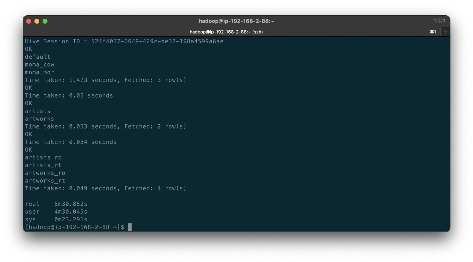
According to documentation, Hudi creates two tables in the Hive metastore for the MoR table type. The first, a table which is a read-optimized view appended with _ro and the second, a table with the same name appended with _rt which is a real-time view. According to Hudi, the read-optimized view exposes columnar Parquet while the real-time view exposes columnar Parquet and/or row-based logs; you can query both tables. The CoW table type creates a single table without a suffix for each datasource (e.g., artists). Below, we see the Hive table structure for the artists_rt table, created by DeltaStreamer, using SHOW CREATE TABLE moma_mor.artists_rt;.
Having run the demonstration’s deltastreamer_jobs_bulk_bkgd.sh script, the resulting object structure in the Hudi-managed section of the Amazon S3 bucket looks as follows.

Below is an example of Hudi files created in the /moma/artists_cow/ S3 object prefix. When using data lake table formats like Hudi, given its specialized directory structure and the high number of objects, interactions with the data should be abstracted through Hudi’s programming interfaces. Generally speaking, you do not interact directly with the objects in a data lake.
Hudi CLI
Optionally, we can inspect the Hudi tables using the Hudi CLI (hudi-cli). The CLI offers an extensive list of available commands. Using the CLI, we can inspect the Hudi tables and their schemas, and review operational statistics like write amplification (the number of bytes written for 1 byte of incoming data), commits, and compactions.
The following short video-only clip shows the use of the Hudi CLI, running on the Amazon EMR Master Node, to inspect the Hudi tables in S3.
Hudi Data Structure
Recall the sample Kafka message we saw earlier in the post representing an insert of an artist record with the artist_id 1. Below, we see what the same record looks like after being ingested by Hudi DeltaStreamer. Note the five additional fields added by Hudi with the _hoodie_ prefix.
Querying Hudi-managed Data
With the initial data ingestion complete and the CDC and DeltaStreamer processes monitoring for future changes, we can query the resulting data stored in Hudi tables. First, we will make some changes to the PostgreSQL MoMA Collection database to see how Hudi manages the data mutations. We could also make changes directly to the Hudi tables using Hive, Spark, or Presto. However, that would cause our datasource to be out of sync with the Hudi tables, potentially negating the entire CDC process. When developing a data lake, this is a critically important consideration — how changes are introduced to Hudi tables, especially when CDC is involved, and whether data continuity between datasources and the data lake is essential.
For the demonstration, I have made a series of arbitrary updates to a piece of artwork in the MoMA Collection database, ‘Picador (La Pique)’ by Pablo Picasso.
Below, note the last four objects shown in S3. Judging by the file names and dates, we can see that the CDC process, using Kafka Connect, has picked up the four updates I made to the record in the database. The Source Connector first wrote the changes to Kafka. The Sink Connector then read those Kafka messages and wrote the data to Amazon S3 in Avro format, as shown below.

Looking again at S3, we can also observe that DeltaStreamer picked up the new CDC objects in Amazon S3 and wrote them to both the Hudi CoW and MoR tables. Note the file types shown below. Given Hudi’s MoR table type structure, Hudi first logged the changes to row-based delta files and later compacted them to produce a new version of the columnar-format Parquet file.

Querying Results from Apache Hive
There are several ways to query Hudi-managed data in S3. In this demonstration, they include against Apache Hive using the hive client from the command line, against Hive using Spark, and against the Hudi tables also using Spark. We could also install Presto on EMR to query the Hudi data directly or via Hive.
Querying the real-time artwork_rt table in Hive after we make each database change, we can observe the data in Hudi reflects the updates. Note that the value of the _hoodie_file_name field for the first three updates is a Hudi delta log file, while the value for the last update is a Parquet file. The Parquet file signifies compaction occurred between the fourth update was made, and the time the Hive query was executed. Lastly, note the type of operation (_op) indicates an update change (u) for all records.

Once all fours database updates are complete and compaction has occurred, we should observe identical results from all Hive tables. Below, note the _hoodie_file_name field for all three tables is a Parquet file. Logically, the Parquet file for the MoR read-optimized and real-time Hive tables is the same.

Had we queried the data previous to compaction, the results would have differed. Below we have three queries. I further updated the artwork record, changing the date field from 1959 to 1960. The read-optimized MoR table, artworks_ro, still reflects the original date value, 1959, before the update and prior to compaction. The real-time table,artworks_rt , reflects the latest update to the date field, 1960. Note that the value of the _hoodie_file_name field for the read-optimized table is a Parquet file, while the value for the real-time table (artworks_rt), the third and final query, is a delta log file. The delta log allows the real-time table to display the most current state of the data in Hudi.

Below are a few useful Hive commands to query the changes in Hudi.
Deletes with Hudi
In addition to inserts and updates (upserts), Apache Hudi can manage deletes. Hudi supports implementing two types of deletes on data stored in Hudi tables: soft deletes and hard deletes. Given this demonstration’s specific configuration for CDC and DeltaStreamer, we will use soft deletes. Soft deletes retain the record key and nullify the other field’s values. Hard deletes, a stronger form of deletion, physically remove any record trace from the Hudi table.
Below, we see the CDC record for the artist with artist_id 441. The event flattening single message transformation (SMT), used by the Debezium-based Kafka Connect Source Connector, adds the __deleted field with a value of true and nullifies all fields except the record’s key, artist_id, which is required.
Below, we see the same delete record for the artist with artist_id 441 in the Hudi MoR table. All the null fields have been removed.
Below, we see how the deleted record appears in the three Hive CoW and MoR artwork tables. Note the query results from the read-optimized MoR table, artworks_ro, contains two records — the original record (r) and the deleted record (d). The data is partitioned by nationality, and since the record was deleted, the nationality field is changed to null. In S3, Hudi represents this partition as nationality=default. The record now exists in two different Parquet files, within two separate partitions, something to be aware of when querying the read-optimized MoR table.

Time Travel
According to the documentation, Hudi has supported time travel queries since version 0.9.0. With time travel, you can query the previous state of your data. Time travel is particularly useful for use cases, including rollbacks, debugging, and audit history.
To demonstrate time travel queries in Hudi, we start by making some additional changes to the source database. For this demonstration, I made a series of five updates and finally a delete to the artist record with artist_id 299 in the PostgreSQL database over a few-hour period.
Once the CDC and DeltaStreamer ingestion processes are complete, we can use Hudi’s time travel query capability to view the state of data in Hudi at different points in time (instants). To do so, we need to provide an as.an.instant date/time value to Spark (see line 21 below).
Based on the time period in which I made the five updates and the delete, I have chosen six instants during that period where I want to examine the state of the record. Below is an example of the PySpark code from a Jupyter Notebook used to perform the six time travel queries against the Hudi MoR artist’s table.
Below, we see the results of the time travel queries. At each instant, we can observe the mutating state of the data in the Hudi MoR Artist’s table, including the initial bulk insert of the existing snapshot of data (r) and the delete record (d). Since the delete made in the PostgreSQL database was recorded as a soft delete in Hudi, as opposed to a hard delete, we are still able to retrieve the record at any instant.
In addition to time travel queries, Hudi also offers incremental queries and point in time queries.
Conclusion
Although this post only scratches the surface of the capabilities of Debezium and Hudi, you can see the power of CDC using Kafka Connect and Debezium, combined with Hudi, to build and manage open data lakes on AWS.
This blog represents my own viewpoints and not of my employer, Amazon Web Services (AWS). All product names, logos, and brands are the property of their respective owners.
Video Demonstration: Building a Data Lake with Apache Airflow
Posted by Gary A. Stafford in Analytics, AWS, Big Data, Build Automation, Cloud, Python on November 12, 2021
Build a simple Data Lake on AWS using a combination of services, including Amazon Managed Workflows for Apache Airflow (Amazon MWAA), AWS Glue, AWS Glue Studio, Amazon Athena, and Amazon S3
Introduction
In the following video demonstration, we will build a simple data lake on AWS using a combination of services, including Amazon Managed Workflows for Apache Airflow (Amazon MWAA), AWS Glue Data Catalog, AWS Glue Crawlers, AWS Glue Jobs, AWS Glue Studio, Amazon Athena, Amazon Relational Database Service (Amazon RDS), and Amazon S3.
Using a series of Airflow DAGs (Directed Acyclic Graphs), we will catalog and move data from three separate data sources into our Amazon S3-based data lake. Once in the data lake, we will perform ETL (or more accurately ELT) on the raw data — cleansing, augmenting, and preparing it for data analytics. Finally, we will perform aggregations on the refined data and write those final datasets back to our data lake. The data lake will be organized around the data lake pattern of bronze (aka raw), silver (aka refined), and gold (aka aggregated) data, popularized by Databricks.

Demonstration
Source Code
The source code for this demonstration, including the Airflow DAGs, SQL files, and data files, is open-sourced and located on GitHub.
DAGs
The DAGs shown in the video demonstration have been renamed for easier project management within the Airflow UI. The DAGs included in the GitHub project are as follows:
- data_lake__01_clean_and_prep_demo.py
- data_lake__02_run_glue_crawlers_source.py
- data_lake__03_run_glue_jobs_raw.py
- data_lake__04_run_glue_jobs_refined.py
- data_lake__05_submit_athena_queries_agg.py
- data_lake__06_run_dags_01_to_05.py
This blog represents my own viewpoints and not of my employer, Amazon Web Services (AWS). All product names, logos, and brands are the property of their respective owners.
Video Demonstration: Building a Data Lake on AWS
Build a simple Data Lake on AWS using a combination of services, including AWS Glue, AWS Glue Studio, Amazon Athena, and Amazon S3
Introduction
In the following video demonstration, we will build a simple data lake on AWS using a combination of services, including AWS Glue Data Catalog, AWS Glue Crawlers, AWS Glue Jobs, AWS Glue Studio, Amazon Athena, Amazon Relational Database Service (Amazon RDS), and Amazon S3.
We will catalog and move data from three separate data sources into our Amazon S3-based data lake. Once in the data lake, we will perform ETL (or more accurately ELT) on the raw data — cleansing, augmenting, and preparing it for data analytics. Finally, we will perform aggregations on the refined data and write those final datasets back to our data lake. The data lake will be organized around the data lake pattern of bronze (aka raw), silver (aka refined), and gold (aka aggregated) data, popularized by Databricks.
Demonstration
Source Code
The source code for this demonstration, including the SQL statements, is open-sourced and located on GitHub.
This blog represents my own viewpoints and not of my employer, Amazon Web Services (AWS). All product names, logos, and brands are the property of their respective owners.
Employing Amazon Macie to Discover and Protect Sensitive Data in your Amazon S3-based Data Lake
Posted by Gary A. Stafford in AWS, Bash Scripting, Big Data, Cloud, Enterprise Software Development, Python on March 15, 2021
Introduction
Working with Analytics customers, it’s not uncommon to see data lakes with a dozen or more discrete data sources. Data typically originates from sources both internal and external to the customer. Internal data may come from multiple teams, departments, divisions, and enterprise systems. External data comes from vendors, partners, public sources, and subscriptions to licensed data sources. The volume, velocity, variety, veracity, and method of delivery vary across the data sources. All this data is being fed into data lakes for purposes such as analytics, business intelligence, and machine learning.
Given the growing volumes of incoming data and variations amongst data sources, it is increasingly complex, expensive, and time-consuming for organizations to ensure compliance with relevant laws, policies, and regulations. Regulations that impact how data is handled in a data lake include the Organizations Health Insurance Portability and Accountability Act (HIPAA), General Data Privacy Regulation (GDPR), Payment Card Industry Data Security Standard (PCI DSS), California Consumer Privacy Act (CCPA), and the Federal Information Security Management Act (FISMA).
Data Lake
AWS defines a data lake as a centralized repository that allows you to store all your structured and unstructured data at any scale. Once in the data lake, you run different types of analytics — from dashboards and visualizations to big data processing, real-time analytics, and machine learning to guide better decisions.
Data in a data lake is regularly organized or separated by its stage in the analytics process. Incoming data is often referred to as raw data. Data is then processed — cleansed, filtered, enriched, and tokenized if necessary. Lastly, the data is analyzed and aggregated, and the results are written back to the data lake. The analyzed and aggregated data is used to build business intelligence dashboards and reports, machine learning models, and is delivered to downstream or external systems. The different categories of data — raw, processed, and aggregated, are frequently referred to as bronze, silver, and gold, a reference to their overall data quality or value.
Protecting the Data Lake
Imagine you’ve received a large volume of data from an external data source. The incoming data is cleansed, filtered, and enriched. The data is re-formatted, partitioned, compressed for analytical efficiency, and written back to the data lake. Your analytics pipelines run complex and time-consuming queries against the data. Unfortunately, while building reports for a set of stakeholders, you realize that the original data accidentally included credit card information and other sensitive information about your customers. In addition to being out of compliance, you have the wasted time and expense of the initial data processing, as well as the extra time and expense to replace and re-process the data. The solution — Amazon Macie.
Amazon Macie
According to AWS, Amazon Macie is a fully managed data security and data privacy service that uses machine learning and pattern matching to discover and protect your sensitive data stored in Amazon Simple Storage Service (Amazon S3). Macie’s alerts, or findings, can be searched, filtered, and sent to Amazon EventBridge, formerly called Amazon CloudWatch Events, for easy integration with existing workflow or event management systems, or to be used in combination with AWS services, such as AWS Step Functions or Amazon Managed Workflows for Apache Airflow (MWAA) to take automated remediation actions.

Data Discovery and Protection
In this post, we will deploy an automated data inspection workflow to examine sample data in an S3-based data lake. Amazon Macie will examine data files uploaded to an encrypted S3 bucket. If sensitive data is discovered within the files, the files will be moved to an encrypted isolation bucket for further investigation. Email and SMS text alerts will be sent. This workflow will leverage Amazon EventBridge, Amazon Simple Notification Service (Amazon SNS), AWS Lambda, and AWS Systems Manager Parameter Store.

Source Code
Using this git clone command, download a copy of this post’s GitHub repository to your local environment.
git clone --branch main --single-branch --depth 1 --no-tags \
    https://github.com/garystafford/macie-demo.git
AWS resources for this post can be deployed using AWS CloudFormation. To follow along, you will need recent versions of Python 3, Boto3, and the AWS CLI version 2, installed.
Sample Data
We will use synthetic patient data, freely available from the MITRE Corporation. The data was generated by Synthea, MITRE’s open-source, synthetic patient generator that models the medical history of synthetic patients. Synthea data is exported in a variety of data standards, including HL7 FHIR, C-CDA, and CSV. We will use CSV-format data files for this post. Download and unzip the CSV files from the Synthea website.
REMOTE_FILE="synthea_sample_data_csv_apr2020.zip"
wget "https://storage.googleapis.com/synthea-public/${REMOTE_FILE}"
unzip -j "${REMOTE_FILE}" -d synthea_data/
The sixteen CSV data files contain a total of 471,852 rows of data, including column headers.
> wc -l *.csv

      598 allergies.csv
    3,484 careplans.csv
    8,377 conditions.csv
       79 devices.csv
   53,347 encounters.csv
      856 imaging_studies.csv
   15,479 immunizations.csv
   42,990 medications.csv
  299,698 observations.csv
    1,120 organizations.csv
    1,172 patients.csv
    3,802 payer_transitions.csv
       11 payers.csv
   34,982 procedures.csv
    5,856 providers.csv
        1 supplies.csv
  ------------------------------
  471,852 total
Amazon Macie Custom Data Identifier
To demonstrate some of the advanced features of Amazon Macie, we will use three Custom Data Identifiers. According to Macie’s documentation, a custom data identifier is a set of criteria that you define that reflects your organization’s particular proprietary data — for example, employee IDs, customer account numbers, or internal data classifications. We will create three custom data identifiers to detect the specific Synthea-format Patient ID, US driver number, and US passport number columns.

The custom data identifiers in this post use a combination of regular expressions (regex) and keywords. The identifiers are designed to work with structured data, such as CSV files. Macie reports text that matches the regex pattern if any of these keywords are in the name of the column or field that stores the text, or if the text is within the maximum match distance of one of these words in a field value. Macie supports a subset of the regex pattern syntax provided by the Perl Compatible Regular Expressions (PCRE) library.

Enable Macie
Before creating a CloudFormation stack with this demonstration’s resources, you will need to enable Amazon Macie from the AWS Management Console, or use the macie2 API and the AWS CLI with the enable-macie command.
aws macie2 enable-macie
Macie can also be enabled for your multi-account AWS Organization. The enable-organization-admin-account command designates an account as the delegated Amazon Macie administrator account for an AWS organization. For more information, see Managing multiple accounts in Amazon Macie.
AWS_ACCOUNT=111222333444
aws macie2 enable-organization-admin-account \
    --admin-account-id ${AWS_ACCOUNT}
CloudFormation Stack
To create the CloudFormation stack with the supplied template, cloudformation/macie_demo.yml, run the following AWS CLI command. You will need to include an email address and phone number as input parameters. These parameter values will be used to send email and text alerts when Macie produces a sensitive data finding.
Please make sure you understand all the potential cost and security implications of creating the CloudFormation stack before continuing.
SNS_PHONE="+12223334444"
SNS_EMAIL="your-email-address@email.com"

aws cloudformation create-stack \
  --stack-name macie-demo \
  --template-body file://cloudformation/macie_demo.yml \
  --parameters ParameterKey=SNSTopicEndpointSms,ParameterValue=${SNS_PHONE} \
  ParameterKey=SNSTopicEndpointEmail,ParameterValue=${SNS_EMAIL} \
  --capabilities CAPABILITY_NAMED_IAM
As shown in the AWS CloudFormation console, the new macie-demo stack will contain twenty-one AWS resources.

Upload Data
Next, with the stack deployed, upload the CSV format data files to the encrypted S3 bucket, representing your data lake. The target S3 bucket has the following naming convention, synthea-data-<aws_account_id>-<region>. You can retrieve the two new bucket names from AWS Systems Manager Parameter Store, which were written there by CloudFormation, using the ssm API.
aws ssm get-parameters-by-path \
  --path /macie_demo/ \
  --query 'Parameters[*].Value'
Use the following ssm and s3 API commands to upload the data files.
DATA_BUCKET=$(aws ssm get-parameter \
    --name /macie_demo/patient_data_bucket \
    --query 'Parameter.Value')
aws s3 cp synthea_data/ \
    "s3://$(eval echo ${DATA_BUCKET})/patient_data/" --recursive
You should end up with sixteen CSV files in the S3 bucket, totaling approximately 82.3 MB.

Sensitive Data Discovery Jobs
With the CloudFormation stack created and the patient data files uploaded, we will create two sensitive data discovery jobs. These jobs will scan the contents of the encrypted S3 bucket for sensitive data and report the findings. According to the documentation, you can configure a sensitive data discovery job to run only once for on-demand analysis and assessment, or on a recurring basis for periodic analysis, assessment, and monitoring. For this demonstration, we will create a one-time sensitive data discovery job using the AWS CLI. We will also create a recurring sensitive data discovery job using the AWS SDK for Python (Boto3). Both jobs can also be created from within Macie’s Jobs console.

For both sensitive data discovery jobs, we will include the three custom data identifiers. Each of the custom data identifiers has a unique ID. We will need all three IDs to create the two sensitive data discovery jobs. You can use the AWS CLI and the macie2 API to retrieve the values.
aws macie2 list-custom-data-identifiers --query 'items[*].id'
Next, modify the job_specs/macie_job_specs_1x.json file, adding the three custom data identifier IDs. Also, update your AWS account ID and S3 bucket name (lines 3–5, 12, and 14). Note that since all the patient data files are in CSV format, we will limit our inspection to only files with a csv file extension (lines 18–33).
The above JSON template was generated using the standard AWS CLI generate-cli-skeleton command.
aws macie2 create-classification-job --generate-cli-skeleton
To create a one-time sensitive data discovery job using the above JSON template, run the following AWS CLI command. The unique job name will be dynamically generated based on the current time.
aws macie2 create-classification-job \
    --name $(echo "SyntheaPatientData_${EPOCHSECONDS}") \
    --cli-input-json file://job_specs/macie_job_specs_1x.json
In the Amazon Macie Jobs console, we can see a one-time sensitive data discovery job running. With a sampling depth of 100, the job will take several minutes to run. The samplingPercentage job property can be adjusted to scan any percentage of the data. If this value is less than 100, Macie selects the objects to analyze at random, up to the specified percentage and analyzes all the data in those objects.

Once the job is completed, the findings will be available in Macie’s Findings console. Using the three custom data identifiers in addition to Macie’s managed data identifiers, there should be a total of fifteen findings from the Synthea patient data files in S3. There should be six High severity findings and nine Medium severity findings. Of those, three are of a Personal finding type, seven of a Custom Identifier finding type, and five of a Multiple finding type, having both Personal and Custom Identifier finding types.

Isolating High Severity Findings
The data inspection workflow we have deployed uses an AWS Lambda function, macie-object-mover, to isolate all data files with High severity findings to a second S3 bucket. The offending files are copied to the isolation bucket and deleted from the source bucket.
Amazon EventBridge
According to Macie’s documentation, to support integration with other applications, services, and systems, such as monitoring or event management systems, Amazon Macie automatically publishes findings to Amazon EventBridge as finding events. Amazon EventBridge is a serverless event bus that makes it easier to build event-driven applications at scale using events generated from your applications, integrated Software-as-a-Service (SaaS) applications, and AWS services.
Each EventBridge rule contains an event pattern. The event pattern is used to filter the incoming stream of events for particular patterns. The EventBridge rule that is triggered when a Macie finding is based on any of the custom data identifiers, macie-rule-custom, uses the event pattern shown below. This pattern examines the finding event for the name of one of the three custom data identifier names that triggered it.

Each EventBridge rule contains an event pattern. The event pattern is used to filter the incoming stream of events for particular patterns. The EventBridge rule that is triggered when a Macie finding is based on one of the three custom data identifiers, macie-rule-high, uses the event pattern shown below. This pattern examines the finding event for the name of one of the three custom data identifier names that triggered it.
{
  "source": [
    "aws.macie"
  ],
  "detail-type": [
    "Macie Finding"
  ],
  "detail": {
    "classificationDetails": {
      "result": {
        "customDataIdentifiers": {
          "detections": {
            "name": [
              "Patient ID",
              "US Passport",
              "US Driver License"
            ]
          }
        }
      }
    }
  }
}
Six data files, containing High severity findings, will be moved to the isolation bucket by the Lambda, triggered by EventBridge.

Scheduled Sensitive Data Discovery Jobs
Data sources commonly deliver data on a repeated basis, such as nightly data feeds. For these types of data sources, we can schedule sensitive data discovery jobs to run on a scheduled basis. For this demonstration, we will create a scheduled job using the AWS SDK for Python (Boto3). Unlike the AWS CLI-based one-time job, you don’t need to modify the project’s script, scripts/create_macie_job_daily.py. The Python script will retrieve your AWS account ID and three custom data identifier IDs. The Python script then runs the create_classification_job command.
To create the scheduled sensitive data discovery job, run the following command.
python3 ./scripts/create_macie_job_daily.py
The scheduleFrequency parameter is set to { 'dailySchedule': {} }. This value specifies a daily recurrence pattern for running the job. The initialRun parameter of the create_classification_job command is set to True. This will cause the new job to analyze all eligible objects immediately after the job is created, in addition to on a daily basis.

Conclusion
In this post, we learned how we can use Amazon Macie to discover and protect sensitive data in Amazon S3. We learned how to use automation to trigger alerts based on Macie’s findings and to isolate data files based on the types of findings. The post’s data inspection workflow can easily be incorporated into existing data lake ingestion pipelines to ensure the integrity of incoming data.
This blog represents my own viewpoints and not of my employer, Amazon Web Services (AWS). All product names, logos, and brands are the property of their respective owners.
Getting Started with Data Analysis on AWS using AWS Glue, Amazon Athena, and QuickSight: Part 2
Posted by Gary A. Stafford in AWS, Big Data, Cloud, Software Development, SQL on January 14, 2020
Introduction
In part one, we learned how to ingest, transform, and enrich raw, semi-structured data, in multiple formats, using Amazon S3, AWS Glue, Amazon Athena, and AWS Lambda. We built an S3-based data lake and learned how AWS leverages open-source technologies, including Presto, Apache Hive, and Apache Parquet. In part two of this post, we will use the transformed and enriched data sources, stored in the data lake, to create compelling visualizations using Amazon QuickSight.
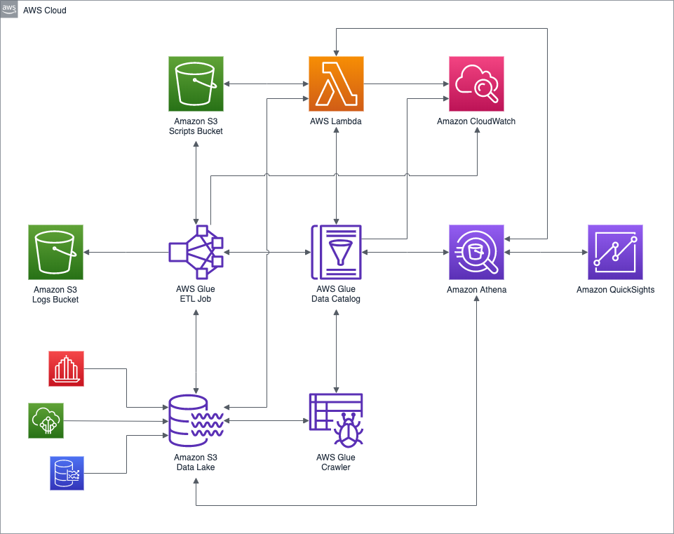 High-level AWS architecture diagram of the demonstration.
Background
If you recall the demonstration from part one of the post, we had adopted the persona of a large, US-based electric energy provider. The energy provider had developed and sold its next-generation Smart Electrical Monitoring Hub (Smart Hub) to residential customers. Customers can analyze their electrical usage with a fine level of granularity, per device and over time. The goal of the Smart Hub is to enable the customers, using data, to reduce their electrical costs. The provider benefits from a reduction in load on the existing electrical grid and a better distribution of daily electrical load as customers shift usage to off-peak times to save money.
Data Visualization and BI
The data analysis process in the demonstration was divided into four logical stages: 1) Raw Data Ingestion, 2) Data Transformation, 3) Data Enrichment, and 4) Data Visualization and Business Intelligence (BI).
 Full data analysis workflow diagram (click to enlarge…)
In the final, Data Visualization and Business Intelligence (BI) stage, the enriched data is presented and analyzed. There are many enterprise-grade services available for data visualization and business intelligence, which integrate with Amazon Athena. Amazon services include Amazon QuickSight, Amazon EMR, and Amazon SageMaker. Third-party solutions from AWS Partners, many available on the AWS Marketplace, include Tableau, Looker, Sisense, and Domo.
In this demonstration, we will focus on Amazon QuickSight. Amazon QuickSight is a fully managed business intelligence (BI) service. QuickSight lets you create and publish interactive dashboards that include ML Insights. Dashboards can be accessed from any device, and embedded into your applications, portals, and websites. QuickSight serverlessly scales automatically from tens of users to tens of thousands without any infrastructure management.
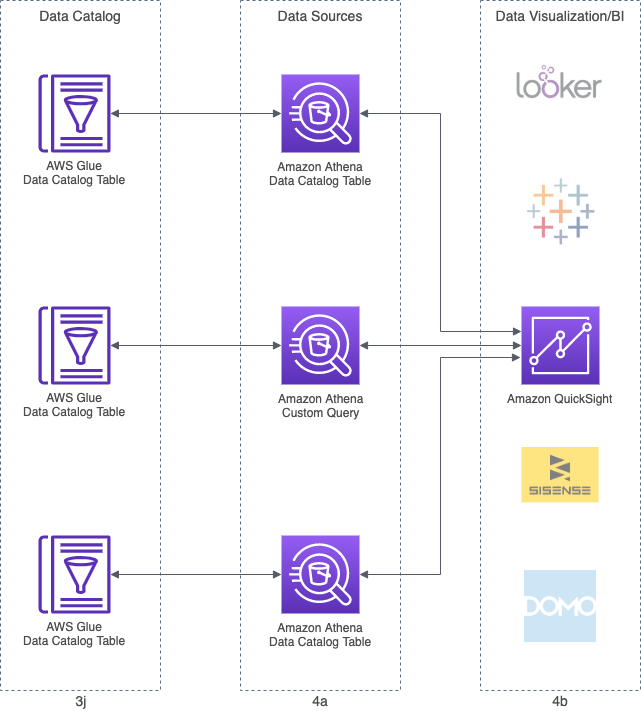
Using QuickSight
QuickSight APIs
Amazon recently added a full set of aws quicksight APIs for interacting with QuickSight. For example, to preview the three QuickSight data sets created for this part of the demo, with the AWS CLI, we would use the list-data-sets comand.
This file contains bidirectional Unicode text that may be interpreted or compiled differently than what appears below. To review, open the file in an editor that reveals hidden Unicode characters.
Learn more about bidirectional Unicode characters
| aws quicksight list-data-sets –aws-account-id 123456789012 |
This file contains bidirectional Unicode text that may be interpreted or compiled differently than what appears below. To review, open the file in an editor that reveals hidden Unicode characters.
Learn more about bidirectional Unicode characters
| { | |
| "Status": 200, | |
| "DataSetSummaries": [ | |
| { | |
| "Arn": "arn:aws:quicksight:us-east-1:123456789012:dataset/9eb88a69-20de-d8be-aefd-2c7ac4e23748", | |
| "DataSetId": "9eb88a69-20de-d8be-aefd-2c7ac4e23748", | |
| "Name": "etl_output_parquet", | |
| "CreatedTime": 1578028774.897, | |
| "LastUpdatedTime": 1578955245.02, | |
| "ImportMode": "SPICE" | |
| }, | |
| { | |
| "Arn": "arn:aws:quicksight:us-east-1:123456789012:dataset/78e81193-189c-6dd0-864fb-a33244c9654", | |
| "DataSetId": "78e81193-189c-6dd0-864fb-a33244c9654", | |
| "Name": "electricity_rates_parquet", | |
| "CreatedTime": 1578029224.996, | |
| "LastUpdatedTime": 1578945179.472, | |
| "ImportMode": "SPICE" | |
| }, | |
| { | |
| "Arn": "arn:aws:quicksight:us-east-1:123456789012:dataset/a474214d-c838-b384-bcca-ea1fcd2dd094", | |
| "DataSetId": "a474214d-c838-b384-bcca-ea1fcd2dd094", | |
| "Name": "smart_hub_locations_parquet", | |
| "CreatedTime": 1578029124.565, | |
| "LastUpdatedTime": 1578888788.135, | |
| "ImportMode": "SPICE" | |
| } | |
| ], | |
| "RequestId": "2524e80c-7c67-7fbd-c3f1-b700c521badc" | |
| } |
To examine details of a single data set, with the AWS CLI, we would use the describe-data-set command.
This file contains bidirectional Unicode text that may be interpreted or compiled differently than what appears below. To review, open the file in an editor that reveals hidden Unicode characters.
Learn more about bidirectional Unicode characters
| aws quicksight describe-data-set \ | |
| –aws-account-id 123456789012 \ | |
| –data-set-id 9eb88a69-20de-d8be-aefd-2c7ac4e23748 |
QuickSight Console
However, for this final part of the demonstration, we will be working from the Amazon QuickSight Console, as opposed to the AWS CLI, AWS CDK, or CloudFormation templates.
Signing Up for QuickSight
To use Amazon QuickSight, you must sign up for QuickSight.

There are two Editions of Amazon QuickSight, Standard and Enterprise. For this demonstration, the Standard Edition will suffice.

QuickSight Data Sets
Amazon QuickSight uses Data Sets as the basis for all data visualizations. According to AWS, QuickSight data sets can be created from a wide variety of data sources, including Amazon RDS, Amazon Aurora, Amazon Redshift, Amazon Athena, and Amazon S3. You can also upload Excel spreadsheets or flat files (CSV, TSV, CLF, ELF, and JSON), connect to on-premises databases like SQL Server, MySQL, and PostgreSQL and import data from SaaS applications like Salesforce. Below, we see a list of the latest data sources available in the QuickSight New Data Set Console.

Demonstration Data Sets
For the demonstration, I have created three QuickSight data sets, all based on Amazon Athena. You have two options when using Amazon Athena as a data source. The first option is to select a table from an AWS Glue Data Catalog database, such as the database we created in part one of the post, ‘smart_hub_data_catalog.’ The second option is to create a custom SQL query, based on one or more tables in an AWS Glue Data Catalog database.

Of the three data sets created for part two of this demonstration, two data sets use tables directly from the Data Catalog, including ‘etl_output_parquet’ and ‘electricity_rates_parquet.’ The third data set uses a custom SQL query, based on the single Data Catalog table, ‘smart_hub_locations_parquet.’ All three tables used to create the data sets represent the enriched, highly efficient Parquet-format data sources in the S3-based Data Lake.

Data Set Features
There are a large number of features available when creating and configuring data sets. We cannot possibly cover all of them in this post. Let’s look at three features: geospatial field types, calculated fields, and custom SQL.
Geospatial Data Types
QuickSight can intelligently detect common types of geographic fields in a data source and assign QuickSight geographic data type, including Country, County, City, Postcode, and State. QuickSight can also detect geospatial data, including Latitude and Longitude. We will take advantage of this QuickSight feature for our three data set’s data sources, including the State, Postcode, Latitude, and Longitude field types.

Calculated Fields
A commonly-used QuickSight data set feature is the ‘Calculated field.’ For the ‘etl_output_parquet’ data set, I have created a new field (column), cost_dollar.

The cost field is the electrical cost of the device, over a five minute time interval, in cents (¢). The calculated cost_dollar field is the quotient of the cost field divided by 100. This value represents the electrical cost of the device, over a five minute time interval, in dollars ($). This is a straightforward example. However, a calculated field can be very complex, built from multiple arithmetic, comparison, and conditional functions, string calculations, and data set fields.

Data set calculated fields can also be created and edited from the QuickSight Analysis Console (discussed later).

Custom SQL
The third QuickSight data set is based on an Amazon Athena custom SQL query.
This file contains bidirectional Unicode text that may be interpreted or compiled differently than what appears below. To review, open the file in an editor that reveals hidden Unicode characters.
Learn more about bidirectional Unicode characters
| SELECT lon, lat, postcode, hash, tz, state | |
| FROM smart_hub_data_catalog.smart_hub_locations_parquet; |
Although you can write queries in the QuickSight Data Prep Console, I prefer to write custom Athena queries using the Athena Query Editor. Using the Editor, you can write, run, debug, and optimize queries to ensure they function correctly, first.

The Athena query can then be pasted into the Custom SQL window. Clicking ‘Finish’ in the window is the equivalent of ‘Run query’ in the Athena Query Editor Console. The query runs and returns data.

Similar to the Athena Query Editor, queries executed in the QuickSight Data Prep Console will show up in the Athena History tab, with a /* QuickSight */ comment prefix.

SPICE
You will notice the three QuickSight data sets are labeled, ‘SPICE.’ According to AWS, the acronym, SPICE, stands for ‘Super-fast, Parallel, In-memory, Calculation Engine.’ QuickSight’s in-memory calculation engine, SPICE, achieves blazing fast performance at scale. SPICE automatically replicates data for high availability allowing thousands of users to simultaneously perform fast, interactive analysis while shielding your underlying data infrastructure, saving you time and resources. With the Standard Edition of QuickSight, as the first Author, you get 1 GB of SPICE in-memory data for free.
QuickSight Analysis
The QuickSight Analysis Console is where Analyses are created. A specific QuickSight Analysis will contain a collection of data sets and data visualizations (visuals). Each visual is associated with a single data set.
Types of QuickSight Analysis visuals include: horizontal and vertical, single and stacked bar charts, line graphs, combination charts, area line charts, scatter plots, heat maps, pie and donut charts, tree maps, pivot tables, gauges, key performance indicators (KPI), geospatial diagrams, and word clouds. Individual visual titles, legends, axis, and other visual aspects can be easily modified. Visuals can contain drill-downs.
A data set’s fields can be modified from within the Analysis Console. Field types and formats, such as date, numeric, currency fields, can be customized for display. The Analysis can include a Title and subtitle. There are some customizable themes available to change the overall look of the Analysis.

Analysis Filters
Data displayed in the visuals can be further shaped using a combination of Filters, Conditional formatting, and Parameters. Below, we see an example of a typical filter based on a range of dates and times. The data set contains two full days’ worth of data. Here, we are filtering the data to a 14-hour peak electrical usage period, between 8 AM and 10 PM on the same day, 12/21/2019.

Drill-Down, Drill-Up, Focus, and Exclude
According to AWS, all visual types except pivot tables offer the ability to create a hierarchy of fields for a visual element. The hierarchy lets you drill down or up to see data at different levels of the hierarchy. Focus allows you to concentrate on a single element within a hierarchy of fields. Exclude allows you to remove an element from a hierarchy of fields. Below, we see an example of all four of these features, available to apply to the ‘Central Air Conditioner’. Since the AC unit is the largest consumer of electricity on average per day, applying these filters to understand its impact on the overall electrical usage may be useful to an analysis. We can also drill down to minutes from hours or up to days from hours.

Example QuickSight Analysis
A QuickSight Analysis is shared by the Analysis Author as a QuickSight Dashboard. Below, we see an example of a QuickSight Dashboard, built and shared for this demonstration. The ‘Residential Electrical Usage Analysis’ is built from the three data sets created earlier. From those data sets, we have constructed several visuals, including a geospatial diagram, donut chart, heat map, KPI, combination chart, stacked vertical bar chart, and line graph. Each visual’s title, layout, and field display has all customized. The data displayed in the visuals have been filtered differently, including by date and time, by customer id (loc_id), and by state. Conditional formatting is used to enhance the visual appearance of visuals, such as the ‘Total Electrical Cost’ KPI.

Conclusion
In part one, we learned how to ingest, transform, and enrich raw, semi-structured data, in multiple formats, using Amazon S3, AWS Glue, Amazon Athena, and AWS Lambda. We built an S3-based data lake and learned how AWS leverages open-source technologies, including Presto, Apache Hive, and Apache Parquet. In part two of this post, we used the transformed and enriched datasets, stored in the data lake, to create compelling visualizations using Amazon QuickSight.
All opinions expressed in this post are my own and not necessarily the views of my current or past employers or their clients.
Getting Started with Data Analysis on AWS using AWS Glue, Amazon Athena, and QuickSight: Part 1
Posted by Gary A. Stafford in AWS, Bash Scripting, Big Data, Cloud, Python, Serverless, Software Development on January 5, 2020
Introduction
According to Wikipedia, data analysis is “a process of inspecting, cleansing, transforming, and modeling data with the goal of discovering useful information, informing conclusion, and supporting decision-making.” In this two-part post, we will explore how to get started with data analysis on AWS, using the serverless capabilities of Amazon Athena, AWS Glue, Amazon QuickSight, Amazon S3, and AWS Lambda. We will learn how to use these complementary services to transform, enrich, analyze, and visualize semi-structured data.
Data Analysis—discovering useful information, informing conclusion, and supporting decision-making. –Wikipedia
In part one, we will begin with raw, semi-structured data in multiple formats. We will discover how to ingest, transform, and enrich that data using Amazon S3, AWS Glue, Amazon Athena, and AWS Lambda. We will build an S3-based data lake, and learn how AWS leverages open-source technologies, such as Presto, Apache Hive, and Apache Parquet. In part two, we will learn how to further analyze and visualize the data using Amazon QuickSight. Here’s a quick preview of what we will build in part one of the post.
Demonstration
In this demonstration, we will adopt the persona of a large, US-based electric energy provider. The energy provider has developed its next-generation Smart Electrical Monitoring Hub (Smart Hub). They have sold the Smart Hub to a large number of residential customers throughout the United States. The hypothetical Smart Hub wirelessly collects detailed electrical usage data from individual, smart electrical receptacles and electrical circuit meters, spread throughout the residence. Electrical usage data is encrypted and securely transmitted from the customer’s Smart Hub to the electric provider, who is running their business on AWS.
Customers are able to analyze their electrical usage with fine granularity, per device, and over time. The goal of the Smart Hub is to enable the customers, using data, to reduce their electrical costs. The provider benefits from a reduction in load on the existing electrical grid and a better distribution of daily electrical load as customers shift usage to off-peak times to save money.
 Preview of post’s data in Amazon QuickSight.
The original concept for the Smart Hub was developed as part of a multi-day training and hackathon, I recently attended with an AWSome group of AWS Solutions Architects in San Francisco. As a team, we developed the concept of the Smart Hub integrated with a real-time, serverless, streaming data architecture, leveraging AWS IoT Core, Amazon Kinesis, AWS Lambda, and Amazon DynamoDB.
 From left: Bruno Giorgini, Mahalingam (‘Mahali’) Sivaprakasam, Gary Stafford, Amit Kumar Agrawal, and Manish Agarwal.
This post will focus on data analysis, as opposed to the real-time streaming aspect of data capture or how the data is persisted on AWS.
High-level AWS architecture diagram of the demonstration.
Featured Technologies
The following AWS services and open-source technologies are featured prominently in this post.

Amazon S3-based Data Lake
 An Amazon S3-based Data Lake uses Amazon S3 as its primary storage platform. Amazon S3 provides an optimal foundation for a data lake because of its virtually unlimited scalability, from gigabytes to petabytes of content. Amazon S3 provides ‘11 nines’ (99.999999999%) durability. It has scalable performance, ease-of-use features, and native encryption and access control capabilities.
AWS Glue
 AWS Glue is a fully managed extract, transform, and load (ETL) service to prepare and load data for analytics. AWS Glue discovers your data and stores the associated metadata (e.g., table definition and schema) in the AWS Glue Data Catalog. Once cataloged, your data is immediately searchable, queryable, and available for ETL.
AWS Glue Data Catalog
 The AWS Glue Data Catalog is an Apache Hive Metastore compatible, central repository to store structural and operational metadata for data assets. For a given data set, store table definition, physical location, add business-relevant attributes, as well as track how the data has changed over time.
AWS Glue Crawler
 An AWS Glue Crawler connects to a data store, progresses through a prioritized list of classifiers to extract the schema of your data and other statistics, and then populates the Glue Data Catalog with this metadata. Crawlers can run periodically to detect the availability of new data as well as changes to existing data, including table definition changes. Crawlers automatically add new tables, new partitions to an existing table, and new versions of table definitions. You can even customize Glue Crawlers to classify your own file types.
AWS Glue ETL Job
An AWS Glue ETL Job is the business logic that performs extract, transform, and load (ETL) work in AWS Glue. When you start a job, AWS Glue runs a script that extracts data from sources, transforms the data, and loads it into targets. AWS Glue generates a PySpark or Scala script, which runs on Apache Spark.
Amazon Athena
 Amazon Athena is an interactive query service that makes it easy to analyze data in Amazon S3 using standard SQL. Athena supports and works with a variety of standard data formats, including CSV, JSON, Apache ORC, Apache Avro, and Apache Parquet. Athena is integrated, out-of-the-box, with AWS Glue Data Catalog. Athena is serverless, so there is no infrastructure to manage, and you pay only for the queries that you run.
The underlying technology behind Amazon Athena is Presto, the open-source distributed SQL query engine for big data, created by Facebook. According to the AWS, the Athena query engine is based on Presto 0.172 (released April 9, 2017). In addition to Presto, Athena uses Apache Hive to define tables.
Amazon QuickSight
 Amazon QuickSight is a fully managed business intelligence (BI) service. QuickSight lets you create and publish interactive dashboards that can then be accessed from any device, and embedded into your applications, portals, and websites.
AWS Lambda
 AWS Lambda automatically runs code without requiring the provisioning or management servers. AWS Lambda automatically scales applications by running code in response to triggers. Lambda code runs in parallel. With AWS Lambda, you are charged for every 100ms your code executes and the number of times your code is triggered. You pay only for the compute time you consume.
Smart Hub Data
Everything in this post revolves around data. For the post’s demonstration, we will start with four categories of raw, synthetic data. Those data categories include Smart Hub electrical usage data, Smart Hub sensor mapping data, Smart Hub residential locations data, and electrical rate data. To demonstrate the capabilities of AWS Glue to handle multiple data formats, the four categories of raw data consist of three distinct file formats: XML, JSON, and CSV. I have attempted to incorporate as many ‘real-world’ complexities into the data without losing focus on the main subject of the post. The sample datasets are intentionally small to keep your AWS costs to a minimum for the demonstration.
To further reduce costs, we will use a variety of data partitioning schemes. According to AWS, by partitioning your data, you can restrict the amount of data scanned by each query, thus improving performance and reducing cost. We have very little data for the demonstration, in which case partitioning may negatively impact query performance. However, in a ‘real-world’ scenario, there would be millions of potential residential customers generating terabytes of data. In that case, data partitioning would be essential for both cost and performance.
Smart Hub Electrical Usage Data
The Smart Hub’s time-series electrical usage data is collected from the customer’s Smart Hub. In the demonstration’s sample electrical usage data, each row represents a completely arbitrary five-minute time interval. There are a total of ten electrical sensors whose electrical usage in kilowatt-hours (kW) is recorded and transmitted. Each Smart Hub records and transmits electrical usage for 10 device sensors, 288 times per day (24 hr / 5 min intervals), for a total of 2,880 data points per day, per Smart Hub. There are two days worth of usage data for the demonstration, for a total of 5,760 data points. The data is stored in JSON Lines format. The usage data will be partitioned in the Amazon S3-based data lake by date (e.g., ‘dt=2019-12-21’).
This file contains bidirectional Unicode text that may be interpreted or compiled differently than what appears below. To review, open the file in an editor that reveals hidden Unicode characters.
Learn more about bidirectional Unicode characters
| {"loc_id":"b6a8d42425fde548","ts":1576915200,"data":{"s_01":0,"s_02":0.00502,"s_03":0,"s_04":0,"s_05":0,"s_06":0,"s_07":0,"s_08":0,"s_09":0,"s_10":0.04167}} | |
| {"loc_id":"b6a8d42425fde548","ts":1576915500,"data":{"s_01":0,"s_02":0.00552,"s_03":0,"s_04":0,"s_05":0,"s_06":0,"s_07":0,"s_08":0,"s_09":0,"s_10":0.04147}} | |
| {"loc_id":"b6a8d42425fde548","ts":1576915800,"data":{"s_01":0.29267,"s_02":0.00642,"s_03":0,"s_04":0,"s_05":0,"s_06":0,"s_07":0,"s_08":0,"s_09":0,"s_10":0.04207}} | |
| {"loc_id":"b6a8d42425fde548","ts":1576916100,"data":{"s_01":0.29207,"s_02":0.00592,"s_03":0,"s_04":0,"s_05":0,"s_06":0,"s_07":0,"s_08":0,"s_09":0,"s_10":0.04137}} | |
| {"loc_id":"b6a8d42425fde548","ts":1576916400,"data":{"s_01":0.29217,"s_02":0.00622,"s_03":0,"s_04":0,"s_05":0,"s_06":0,"s_07":0,"s_08":0,"s_09":0,"s_10":0.04157}} | |
| {"loc_id":"b6a8d42425fde548","ts":1576916700,"data":{"s_01":0,"s_02":0.00562,"s_03":0,"s_04":0,"s_05":0,"s_06":0,"s_07":0,"s_08":0,"s_09":0,"s_10":0.04197}} | |
| {"loc_id":"b6a8d42425fde548","ts":1576917000,"data":{"s_01":0,"s_02":0.00512,"s_03":0,"s_04":0,"s_05":0,"s_06":0,"s_07":0,"s_08":0,"s_09":0,"s_10":0.04257}} | |
| {"loc_id":"b6a8d42425fde548","ts":1576917300,"data":{"s_01":0,"s_02":0.00522,"s_03":0,"s_04":0,"s_05":0,"s_06":0,"s_07":0,"s_08":0,"s_09":0,"s_10":0.04177}} | |
| {"loc_id":"b6a8d42425fde548","ts":1576917600,"data":{"s_01":0,"s_02":0.00502,"s_03":0,"s_04":0,"s_05":0,"s_06":0,"s_07":0,"s_08":0,"s_09":0,"s_10":0.04267}} | |
| {"loc_id":"b6a8d42425fde548","ts":1576917900,"data":{"s_01":0,"s_02":0.00612,"s_03":0,"s_04":0,"s_05":0,"s_06":0,"s_07":0,"s_08":0,"s_09":0,"s_10":0.04237}} |
Note the electrical usage data contains nested data. The electrical usage for each of the ten sensors is contained in a JSON array, within each time series entry. The array contains ten numeric values of type, double.
This file contains bidirectional Unicode text that may be interpreted or compiled differently than what appears below. To review, open the file in an editor that reveals hidden Unicode characters.
Learn more about bidirectional Unicode characters
| { | |
| "loc_id": "b6a8d42425fde548", | |
| "ts": 1576916400, | |
| "data": { | |
| "s_01": 0.29217, | |
| "s_02": 0.00622, | |
| "s_03": 0, | |
| "s_04": 0, | |
| "s_05": 0, | |
| "s_06": 0, | |
| "s_07": 0, | |
| "s_08": 0, | |
| "s_09": 0, | |
| "s_10": 0.04157 | |
| } | |
| } |
Real data is often complex and deeply nested. Later in the post, we will see that AWS Glue can map many common data types, including nested data objects, as illustrated below.

Smart Hub Sensor Mappings
The Smart Hub sensor mappings data maps a sensor column in the usage data (e.g., ‘s_01’ to the corresponding actual device (e.g., ‘Central Air Conditioner’). The data contains the device location, wattage, and the last time the record was modified. The data is also stored in JSON Lines format. The sensor mappings data will be partitioned in the Amazon S3-based data lake by the state of the residence (e.g., ‘state=or’ for Oregon).
This file contains bidirectional Unicode text that may be interpreted or compiled differently than what appears below. To review, open the file in an editor that reveals hidden Unicode characters.
Learn more about bidirectional Unicode characters
| {"loc_id":"b6a8d42425fde548","id":"s_01","description":"Central Air Conditioner","location":"N/A","watts":3500,"last_modified":1559347200} | |
| {"loc_id":"b6a8d42425fde548","id":"s_02","description":"Ceiling Fan","location":"Master Bedroom","watts":65,"last_modified":1559347200} | |
| {"loc_id":"b6a8d42425fde548","id":"s_03","description":"Clothes Dryer","location":"Basement","watts":5000,"last_modified":1559347200} | |
| {"loc_id":"b6a8d42425fde548","id":"s_04","description":"Clothes Washer","location":"Basement","watts":1800,"last_modified":1559347200} | |
| {"loc_id":"b6a8d42425fde548","id":"s_05","description":"Dishwasher","location":"Kitchen","watts":900,"last_modified":1559347200} | |
| {"loc_id":"b6a8d42425fde548","id":"s_06","description":"Flat Screen TV","location":"Living Room","watts":120,"last_modified":1559347200} | |
| {"loc_id":"b6a8d42425fde548","id":"s_07","description":"Microwave Oven","location":"Kitchen","watts":1000,"last_modified":1559347200} | |
| {"loc_id":"b6a8d42425fde548","id":"s_08","description":"Coffee Maker","location":"Kitchen","watts":900,"last_modified":1559347200} | |
| {"loc_id":"b6a8d42425fde548","id":"s_09","description":"Hair Dryer","location":"Master Bathroom","watts":2000,"last_modified":1559347200} | |
| {"loc_id":"b6a8d42425fde548","id":"s_10","description":"Refrigerator","location":"Kitchen","watts":500,"last_modified":1559347200} |
Smart Hub Locations
The Smart Hub locations data contains the geospatial coordinates, home address, and timezone for each residential Smart Hub. The data is stored in CSV format. The data for the four cities included in this demonstration originated from OpenAddresses, ‘the free and open global address collection.’ There are approximately 4k location records. The location data will be partitioned in the Amazon S3-based data lake by the state of the residence where the Smart Hub is installed (e.g., ‘state=or’ for Oregon).
This file contains bidirectional Unicode text that may be interpreted or compiled differently than what appears below. To review, open the file in an editor that reveals hidden Unicode characters.
Learn more about bidirectional Unicode characters
| lon | lat | number | street | unit | city | district | region | postcode | id | hash | tz | |
|---|---|---|---|---|---|---|---|---|---|---|---|---|
| -122.8077278 | 45.4715614 | 6635 | SW JUNIPER TER | 97008 | b6a8d42425fde548 | America/Los_Angeles | ||||||
| -122.8356634 | 45.4385864 | 11225 | SW PINTAIL LOOP | 97007 | 08ae3df798df8b90 | America/Los_Angeles | ||||||
| -122.8252379 | 45.4481709 | 9930 | SW WRANGLER PL | 97008 | 1c7e1f7df752663e | America/Los_Angeles | ||||||
| -122.8354211 | 45.4535977 | 9174 | SW PLATINUM PL | 97007 | b364854408ee431e | America/Los_Angeles | ||||||
| -122.8315771 | 45.4949449 | 15040 | SW MILLIKAN WAY | # 233 | 97003 | 0e97796ba31ba3b4 | America/Los_Angeles | |||||
| -122.7950339 | 45.4470259 | 10006 | SW CONESTOGA DR | # 113 | 97008 | 2b5307be5bfeb026 | America/Los_Angeles | |||||
| -122.8072836 | 45.4908594 | 12600 | SW CRESCENT ST | # 126 | 97005 | 4d74167f00f63f50 | America/Los_Angeles | |||||
| -122.8211801 | 45.4689303 | 7100 | SW 140TH PL | 97008 | c5568631f0b9de9c | America/Los_Angeles | ||||||
| -122.831154 | 45.4317057 | 15050 | SW MALLARD DR | # 101 | 97007 | dbd1321080ce9682 | America/Los_Angeles | |||||
| -122.8162856 | 45.4442878 | 10460 | SW 136TH PL | 97008 | 008faab8a9a3e519 | America/Los_Angeles |
Electrical Rates
Lastly, the electrical rate data contains the cost of electricity. In this demonstration, the assumption is that the rate varies by state, by month, and by the hour of the day. The data is stored in XML, a data export format still common to older, legacy systems. The electrical rate data will not be partitioned in the Amazon S3-based data lake.
This file contains bidirectional Unicode text that may be interpreted or compiled differently than what appears below. To review, open the file in an editor that reveals hidden Unicode characters.
Learn more about bidirectional Unicode characters
| <?xml version="1.0" encoding="UTF-8"?> | |
| <root> | |
| <row> | |
| <state>or</state> | |
| <year>2019</year> | |
| <month>12</month> | |
| <from>19:00:00</from> | |
| <to>19:59:59</to> | |
| <type>peak</type> | |
| <rate>12.623</rate> | |
| </row> | |
| <row> | |
| <state>or</state> | |
| <year>2019</year> | |
| <month>12</month> | |
| <from>20:00:00</from> | |
| <to>20:59:59</to> | |
| <type>partial-peak</type> | |
| <rate>7.232</rate> | |
| </row> | |
| <row> | |
| <state>or</state> | |
| <year>2019</year> | |
| <month>12</month> | |
| <from>21:00:00</from> | |
| <to>21:59:59</to> | |
| <type>partial-peak</type> | |
| <rate>7.232</rate> | |
| </row> | |
| <row> | |
| <state>or</state> | |
| <year>2019</year> | |
| <month>12</month> | |
| <from>22:00:00</from> | |
| <to>22:59:59</to> | |
| <type>off-peak</type> | |
| <rate>4.209</rate> | |
| </row> | |
| </root> |
Data Analysis Process
Due to the number of steps involved in the data analysis process in the demonstration, I have divided the process into four logical stages: 1) Raw Data Ingestion, 2) Data Transformation, 3) Data Enrichment, and 4) Data Visualization and Business Intelligence (BI).
Full data analysis workflow diagram (click to enlarge…)
Raw Data Ingestion
In the Raw Data Ingestion stage, semi-structured CSV-, XML-, and JSON-format data files are copied to a secure Amazon Simple Storage Service (S3) bucket. Within the bucket, data files are organized into folders based on their physical data structure (schema). Due to the potentially unlimited number of data files, files are further organized (partitioned) into subfolders. Organizational strategies for data files are based on date, time, geographic location, customer id, or other common data characteristics.
This collection of semi-structured data files, S3 buckets, and partitions form what is referred to as a Data Lake. According to AWS, a data lake is a centralized repository that allows you to store all your structured and unstructured data at any scale.
A series of AWS Glue Crawlers process the raw CSV-, XML-, and JSON-format files, extracting metadata, and creating table definitions in the AWS Glue Data Catalog. According to AWS, an AWS Glue Data Catalog contains metadata tables, where each table specifies a single data store.

Data Transformation
In the Data Transformation stage, the raw data in the previous stage is transformed. Data transformation may include both modifying the data and changing the data format. Data modifications include data cleansing, re-casting data types, changing date formats, field-level computations, and field concatenation.
The data is then converted from CSV-, XML-, and JSON-format to Apache Parquet format and written back to the Amazon S3-based data lake. Apache Parquet is a compressed, efficient columnar storage format. Amazon Athena, like many Cloud-based services, charges you by the amount of data scanned per query. Hence, using data partitioning, bucketing, compression, and columnar storage formats, like Parquet, will reduce query cost.
Lastly, the transformed Parquet-format data is cataloged to new tables, alongside the raw CSV, XML, and JSON data, in the Glue Data Catalog.

Data Enrichment
According to ScienceDirect, data enrichment or augmentation is the process of enhancing existing information by supplementing missing or incomplete data. Typically, data enrichment is achieved by using external data sources, but that is not always the case.
Data Enrichment—the process of enhancing existing information by supplementing missing or incomplete data. –ScienceDirect
In the Data Enrichment stage, the Parquet-format Smart Hub usage data is augmented with related data from the three other data sources: sensor mappings, locations, and electrical rates. The customer’s Smart Hub usage data is enriched with the customer’s device types, the customer’s timezone, and customer’s electricity cost per monitored period based on the customer’s geographic location and time of day.

Once the data is enriched, it is converted to Parquet and optimized for query performance, stored in the data lake, and cataloged. At this point, the original CSV-, XML-, and JSON-format raw data files, the transformed Parquet-format data files, and the Parquet-format enriched data files are all stored in the Amazon S3-based data lake and cataloged in the Glue Data Catalog.

Data Visualization
In the final Data Visualization and Business Intelligence (BI) stage, the enriched data is presented and analyzed. There are many enterprise-grade services available for visualization and Business Intelligence, which integrate with Athena. Amazon services include Amazon QuickSight, Amazon EMR, and Amazon SageMaker. Third-party solutions from AWS Partners, available on the AWS Marketplace, include Tableau, Looker, Sisense, and Domo. In this demonstration, we will focus on Amazon QuickSight.
Getting Started
Requirements
To follow along with the demonstration, you will need an AWS Account and a current version of the AWS CLI. To get the most from the demonstration, you should also have Python 3 and jq installed in your work environment.
Source Code
All source code for this post can be found on GitHub. Use the following command to clone a copy of the project.
This file contains bidirectional Unicode text that may be interpreted or compiled differently than what appears below. To review, open the file in an editor that reveals hidden Unicode characters.
Learn more about bidirectional Unicode characters
| git clone \ | |
| –branch master –single-branch –depth 1 –no-tags \ | |
| https://github.com/garystafford/athena-glue-quicksight-demo.git |
Source code samples in this post are displayed as GitHub Gists, which will not display correctly on some mobile and social media browsers.
TL;DR?
Just want the jump in without reading the instructions? All the AWS CLI commands, found within the post, are consolidated in the GitHub project’s README file.
CloudFormation Stack
To start, create the ‘smart-hub-athena-glue-stack’ CloudFormation stack using the smart-hub-athena-glue.yml template. The template will create (3) Amazon S3 buckets, (1) AWS Glue Data Catalog Database, (5) Data Catalog Database Tables, (6) AWS Glue Crawlers, (1) AWS Glue ETL Job, and (1) IAM Service Role for AWS Glue.
Make sure to change the DATA_BUCKET, SCRIPT_BUCKET, and LOG_BUCKET variables, first, to your own unique S3 bucket names. I always suggest using the standard AWS 3-part convention of 1) descriptive name, 2) AWS Account ID or Account Alias, and 3) AWS Region, to name your bucket (e.g. ‘smart-hub-data-123456789012-us-east-1’).
This file contains bidirectional Unicode text that may be interpreted or compiled differently than what appears below. To review, open the file in an editor that reveals hidden Unicode characters.
Learn more about bidirectional Unicode characters
| # *** CHANGE ME *** | |
| BUCKET_SUFFIX="123456789012-us-east-1" | |
| DATA_BUCKET="smart-hub-data-${BUCKET_SUFFIX}" | |
| SCRIPT_BUCKET="smart-hub-scripts-${BUCKET_SUFFIX}" | |
| LOG_BUCKET="smart-hub-logs-${BUCKET_SUFFIX}" | |
| aws cloudformation create-stack \ | |
| –stack-name smart-hub-athena-glue-stack \ | |
| –template-body file://cloudformation/smart-hub-athena-glue.yml \ | |
| –parameters ParameterKey=DataBucketName,ParameterValue=${DATA_BUCKET} \ | |
| ParameterKey=ScriptBucketName,ParameterValue=${SCRIPT_BUCKET} \ | |
| ParameterKey=LogBucketName,ParameterValue=${LOG_BUCKET} \ | |
| –capabilities CAPABILITY_NAMED_IAM |
Raw Data Files
Next, copy the raw CSV-, XML-, and JSON-format data files from the local project to the DATA_BUCKET S3 bucket (steps 1a-1b in workflow diagram). These files represent the beginnings of the S3-based data lake. Each category of data uses a different strategy for organizing and separating the files. Note the use of the Apache Hive-style partitions (e.g., /smart_hub_data_json/dt=2019-12-21). As discussed earlier, the assumption is that the actual, large volume of data in the data lake would necessitate using partitioning to improve query performance.
This file contains bidirectional Unicode text that may be interpreted or compiled differently than what appears below. To review, open the file in an editor that reveals hidden Unicode characters.
Learn more about bidirectional Unicode characters
| # location data | |
| aws s3 cp data/locations/denver_co_1576656000.csv \ | |
| s3://${DATA_BUCKET}/smart_hub_locations_csv/state=co/ | |
| aws s3 cp data/locations/palo_alto_ca_1576742400.csv \ | |
| s3://${DATA_BUCKET}/smart_hub_locations_csv/state=ca/ | |
| aws s3 cp data/locations/portland_metro_or_1576742400.csv \ | |
| s3://${DATA_BUCKET}/smart_hub_locations_csv/state=or/ | |
| aws s3 cp data/locations/stamford_ct_1576569600.csv \ | |
| s3://${DATA_BUCKET}/smart_hub_locations_csv/state=ct/ | |
| # sensor mapping data | |
| aws s3 cp data/mappings/ \ | |
| s3://${DATA_BUCKET}/sensor_mappings_json/state=or/ \ | |
| –recursive | |
| # electrical usage data | |
| aws s3 cp data/usage/2019-12-21/ \ | |
| s3://${DATA_BUCKET}/smart_hub_data_json/dt=2019-12-21/ \ | |
| –recursive | |
| aws s3 cp data/usage/2019-12-22/ \ | |
| s3://${DATA_BUCKET}/smart_hub_data_json/dt=2019-12-22/ \ | |
| –recursive | |
| # electricity rates data | |
| aws s3 cp data/rates/ \ | |
| s3://${DATA_BUCKET}/electricity_rates_xml/ \ | |
| –recursive |
Confirm the contents of the DATA_BUCKET S3 bucket with the following command.
This file contains bidirectional Unicode text that may be interpreted or compiled differently than what appears below. To review, open the file in an editor that reveals hidden Unicode characters.
Learn more about bidirectional Unicode characters
| aws s3 ls s3://${DATA_BUCKET}/ \ | |
| –recursive –human-readable –summarize |
There should be a total of (14) raw data files in the DATA_BUCKET S3 bucket.
This file contains bidirectional Unicode text that may be interpreted or compiled differently than what appears below. To review, open the file in an editor that reveals hidden Unicode characters.
Learn more about bidirectional Unicode characters
| 2020-01-04 14:39:51 20.0 KiB electricity_rates_xml/2019_12_1575270000.xml | |
| 2020-01-04 14:39:46 1.3 KiB sensor_mappings_json/state=or/08ae3df798df8b90_1550908800.json | |
| 2020-01-04 14:39:46 1.3 KiB sensor_mappings_json/state=or/1c7e1f7df752663e_1559347200.json | |
| 2020-01-04 14:39:46 1.3 KiB sensor_mappings_json/state=or/b6a8d42425fde548_1568314800.json | |
| 2020-01-04 14:39:47 44.9 KiB smart_hub_data_json/dt=2019-12-21/08ae3df798df8b90_1576915200.json | |
| 2020-01-04 14:39:47 44.9 KiB smart_hub_data_json/dt=2019-12-21/1c7e1f7df752663e_1576915200.json | |
| 2020-01-04 14:39:47 44.9 KiB smart_hub_data_json/dt=2019-12-21/b6a8d42425fde548_1576915200.json | |
| 2020-01-04 14:39:49 44.6 KiB smart_hub_data_json/dt=2019-12-22/08ae3df798df8b90_15770016000.json | |
| 2020-01-04 14:39:49 44.6 KiB smart_hub_data_json/dt=2019-12-22/1c7e1f7df752663e_1577001600.json | |
| 2020-01-04 14:39:49 44.6 KiB smart_hub_data_json/dt=2019-12-22/b6a8d42425fde548_15770016001.json | |
| 2020-01-04 14:39:39 89.7 KiB smart_hub_locations_csv/state=ca/palo_alto_ca_1576742400.csv | |
| 2020-01-04 14:39:37 84.2 KiB smart_hub_locations_csv/state=co/denver_co_1576656000.csv | |
| 2020-01-04 14:39:44 78.6 KiB smart_hub_locations_csv/state=ct/stamford_ct_1576569600.csv | |
| 2020-01-04 14:39:42 91.6 KiB smart_hub_locations_csv/state=or/portland_metro_or_1576742400.csv | |
| Total Objects: 14 | |
| Total Size: 636.7 KiB |
Lambda Functions
Next, package the (5) Python3.8-based AWS Lambda functions for deployment.
This file contains bidirectional Unicode text that may be interpreted or compiled differently than what appears below. To review, open the file in an editor that reveals hidden Unicode characters.
Learn more about bidirectional Unicode characters
| pushd lambdas/athena-json-to-parquet-data || exit | |
| zip -r package.zip index.py | |
| popd || exit | |
| pushd lambdas/athena-csv-to-parquet-locations || exit | |
| zip -r package.zip index.py | |
| popd || exit | |
| pushd lambdas/athena-json-to-parquet-mappings || exit | |
| zip -r package.zip index.py | |
| popd || exit | |
| pushd lambdas/athena-complex-etl-query || exit | |
| zip -r package.zip index.py | |
| popd || exit | |
| pushd lambdas/athena-parquet-to-parquet-elt-data || exit | |
| zip -r package.zip index.py | |
| popd || exit |
Copy the five Lambda packages to the SCRIPT_BUCKET S3 bucket. The ZIP archive Lambda packages are accessed by the second CloudFormation stack, smart-hub-serverless. This CloudFormation stack, which creates the Lambda functions, will fail to deploy if the packages are not found in the SCRIPT_BUCKET S3 bucket.
I have chosen to place the packages in a different S3 bucket then the raw data files. In a real production environment, these two types of files would be separated, minimally, into separate buckets for security. Remember, only data should go into the data lake.
This file contains bidirectional Unicode text that may be interpreted or compiled differently than what appears below. To review, open the file in an editor that reveals hidden Unicode characters.
Learn more about bidirectional Unicode characters
| aws s3 cp lambdas/athena-json-to-parquet-data/package.zip \ | |
| s3://${SCRIPT_BUCKET}/lambdas/athena_json_to_parquet_data/ | |
| aws s3 cp lambdas/athena-csv-to-parquet-locations/package.zip \ | |
| s3://${SCRIPT_BUCKET}/lambdas/athena_csv_to_parquet_locations/ | |
| aws s3 cp lambdas/athena-json-to-parquet-mappings/package.zip \ | |
| s3://${SCRIPT_BUCKET}/lambdas/athena_json_to_parquet_mappings/ | |
| aws s3 cp lambdas/athena-complex-etl-query/package.zip \ | |
| s3://${SCRIPT_BUCKET}/lambdas/athena_complex_etl_query/ | |
| aws s3 cp lambdas/athena-parquet-to-parquet-elt-data/package.zip \ | |
| s3://${SCRIPT_BUCKET}/lambdas/athena_parquet_to_parquet_elt_data/ |
Create the second ‘smart-hub-lambda-stack’ CloudFormation stack using the smart-hub-lambda.yml CloudFormation template. The template will create (5) AWS Lambda functions and (1) Lambda execution IAM Service Role.
This file contains bidirectional Unicode text that may be interpreted or compiled differently than what appears below. To review, open the file in an editor that reveals hidden Unicode characters.
Learn more about bidirectional Unicode characters
| aws cloudformation create-stack \ | |
| –stack-name smart-hub-lambda-stack \ | |
| –template-body file://cloudformation/smart-hub-lambda.yml \ | |
| –capabilities CAPABILITY_NAMED_IAM |
At this point, we have deployed all of the AWS resources required for the demonstration using CloudFormation. We have also copied all of the raw CSV-, XML-, and JSON-format data files in the Amazon S3-based data lake.
AWS Glue Crawlers
If you recall, we created five tables in the Glue Data Catalog database as part of the CloudFormation stack. One table for each of the four raw data types and one table to hold temporary ELT data later in the demonstration. To confirm the five tables were created in the Glue Data Catalog database, use the Glue Data Catalog Console, or run the following AWS CLI / jq command.
This file contains bidirectional Unicode text that may be interpreted or compiled differently than what appears below. To review, open the file in an editor that reveals hidden Unicode characters.
Learn more about bidirectional Unicode characters
| aws glue get-tables \ | |
| –database-name smart_hub_data_catalog \ | |
| | jq -r '.TableList[].Name' |
The five data catalog tables should be as follows.
This file contains bidirectional Unicode text that may be interpreted or compiled differently than what appears below. To review, open the file in an editor that reveals hidden Unicode characters.
Learn more about bidirectional Unicode characters
| electricity_rates_xml | |
| etl_tmp_output_parquet | |
| sensor_mappings_json | |
| smart_hub_data_json | |
| smart_hub_locations_csv |
We also created six Glue Crawlers as part of the CloudFormation template. Four of these Crawlers are responsible for cataloging the raw CSV-, XML-, and JSON-format data from S3 into the corresponding, existing Glue Data Catalog database tables. The Crawlers will detect any new partitions and add those to the tables as well. Each Crawler corresponds to one of the four raw data types. Crawlers can be scheduled to run periodically, cataloging new data and updating data partitions. Crawlers will also create a Data Catalog database tables. We use Crawlers to create new tables, later in the post.
Run the four Glue Crawlers using the AWS CLI (step 1c in workflow diagram).
This file contains bidirectional Unicode text that may be interpreted or compiled differently than what appears below. To review, open the file in an editor that reveals hidden Unicode characters.
Learn more about bidirectional Unicode characters
| aws glue start-crawler –name smart-hub-locations-csv | |
| aws glue start-crawler –name smart-hub-sensor-mappings-json | |
| aws glue start-crawler –name smart-hub-data-json | |
| aws glue start-crawler –name smart-hub-rates-xml |
You can check the Glue Crawler Console to ensure the four Crawlers finished successfully.

Alternately, use another AWS CLI / jq command.
This file contains bidirectional Unicode text that may be interpreted or compiled differently than what appears below. To review, open the file in an editor that reveals hidden Unicode characters.
Learn more about bidirectional Unicode characters
| aws glue get-crawler-metrics \ | |
| | jq -r '.CrawlerMetricsList[] | "\(.CrawlerName): \(.StillEstimating), \(.TimeLeftSeconds)"' \ | |
| | grep "^smart-hub-[A-Za-z-]*" |
When complete, all Crawlers should all be in a state of ‘Still Estimating = false’ and ‘TimeLeftSeconds = 0’. In my experience, the Crawlers can take up one minute to start, after the estimation stage, and one minute to stop when complete.
This file contains bidirectional Unicode text that may be interpreted or compiled differently than what appears below. To review, open the file in an editor that reveals hidden Unicode characters.
Learn more about bidirectional Unicode characters
| smart-hub-data-json: true, 0 | |
| smart-hub-etl-tmp-output-parquet: false, 0 | |
| smart-hub-locations-csv: false, 15 | |
| smart-hub-rates-parquet: false, 0 | |
| smart-hub-rates-xml: false, 15 | |
| smart-hub-sensor-mappings-json: false, 15 |
Successfully running the four Crawlers completes the Raw Data Ingestion stage of the demonstration.
Converting to Parquet with CTAS
With the Raw Data Ingestion stage completed, we will now transform the raw Smart Hub usage data, sensor mapping data, and locations data into Parquet-format using three AWS Lambda functions. Each Lambda subsequently calls Athena, which executes a CREATE TABLE AS SELECT SQL statement (aka CTAS) . Each Lambda executes a similar command, varying only by data source, data destination, and partitioning scheme. Below, is an example of the command used for the Smart Hub electrical usage data, taken from the Python-based Lambda, athena-json-to-parquet-data/index.py.
This file contains bidirectional Unicode text that may be interpreted or compiled differently than what appears below. To review, open the file in an editor that reveals hidden Unicode characters.
Learn more about bidirectional Unicode characters
| query = \ | |
| "CREATE TABLE IF NOT EXISTS " + data_catalog + "." + output_directory + " " \ | |
| "WITH ( " \ | |
| " format = 'PARQUET', " \ | |
| " parquet_compression = 'SNAPPY', " \ | |
| " partitioned_by = ARRAY['dt'], " \ | |
| " external_location = 's3://" + data_bucket + "/" + output_directory + "' " \ | |
| ") AS " \ | |
| "SELECT * " \ | |
| "FROM " + data_catalog + "." + input_directory + ";" |
This compact, yet powerful CTAS statement converts a copy of the raw JSON- and CSV-format data files into Parquet-format, and partitions and stores the resulting files back into the S3-based data lake. Additionally, the CTAS SQL statement catalogs the Parquet-format data files into the Glue Data Catalog database, into new tables. Unfortunately, this method will not work for the XML-format raw data files, which we will tackle next.
The five deployed Lambda functions should be visible from the Lambda Console’s Functions tab.

Invoke the three Lambda functions using the AWS CLI. (part of step 2a in workflow diagram).
This file contains bidirectional Unicode text that may be interpreted or compiled differently than what appears below. To review, open the file in an editor that reveals hidden Unicode characters.
Learn more about bidirectional Unicode characters
| aws lambda invoke \ | |
| –function-name athena-json-to-parquet-data \ | |
| response.json | |
| aws lambda invoke \ | |
| –function-name athena-csv-to-parquet-locations \ | |
| response.json | |
| aws lambda invoke \ | |
| –function-name athena-json-to-parquet-mappings \ | |
| response.json |
Here is an example of the same CTAS command, shown above for the Smart Hub electrical usage data, as it is was executed successfully by Athena.
This file contains bidirectional Unicode text that may be interpreted or compiled differently than what appears below. To review, open the file in an editor that reveals hidden Unicode characters.
Learn more about bidirectional Unicode characters
| CREATE TABLE IF NOT EXISTS smart_hub_data_catalog.smart_hub_data_parquet | |
| WITH (format = 'PARQUET', | |
| parquet_compression = 'SNAPPY', | |
| partitioned_by = ARRAY['dt'], | |
| external_location = 's3://smart-hub-data-demo-account-1-us-east-1/smart_hub_data_parquet') | |
| AS | |
| SELECT * | |
| FROM smart_hub_data_catalog.smart_hub_data_json |
We can view any Athena SQL query from the Athena Console’s History tab. Clicking on a query (in pink) will copy it to the Query Editor tab and execute it. Below, we see the three SQL statements executed by the Lamba functions.
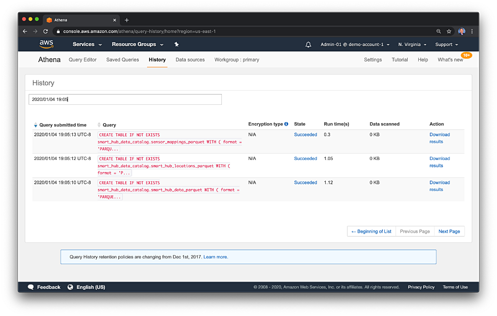
AWS Glue ETL Job for XML
If you recall, the electrical rate data is in XML format. The Lambda functions we just executed, converted the CSV and JSON data to Parquet using Athena. Currently, unlike CSV, JSON, ORC, Parquet, and Avro, Athena does not support the older XML data format. For the XML data files, we will use an AWS Glue ETL Job to convert the XML data to Parquet. The Glue ETL Job is written in Python and uses Apache Spark, along with several AWS Glue PySpark extensions. For this job, I used an existing script created in the Glue ETL Jobs Console as a base, then modified the script to meet my needs.
This file contains bidirectional Unicode text that may be interpreted or compiled differently than what appears below. To review, open the file in an editor that reveals hidden Unicode characters.
Learn more about bidirectional Unicode characters
| import sys | |
| from awsglue.transforms import * | |
| from awsglue.utils import getResolvedOptions | |
| from pyspark.context import SparkContext | |
| from awsglue.context import GlueContext | |
| from awsglue.job import Job | |
| args = getResolvedOptions(sys.argv, [ | |
| 'JOB_NAME', | |
| 's3_output_path', | |
| 'source_glue_database', | |
| 'source_glue_table' | |
| ]) | |
| s3_output_path = args['s3_output_path'] | |
| source_glue_database = args['source_glue_database'] | |
| source_glue_table = args['source_glue_table'] | |
| sc = SparkContext() | |
| glueContext = GlueContext(sc) | |
| spark = glueContext.spark_session | |
| job = Job(glueContext) | |
| job.init(args['JOB_NAME'], args) | |
| datasource0 = glueContext. \ | |
| create_dynamic_frame. \ | |
| from_catalog(database=source_glue_database, | |
| table_name=source_glue_table, | |
| transformation_ctx="datasource0") | |
| applymapping1 = ApplyMapping.apply( | |
| frame=datasource0, | |
| mappings=[("from", "string", "from", "string"), | |
| ("to", "string", "to", "string"), | |
| ("type", "string", "type", "string"), | |
| ("rate", "double", "rate", "double"), | |
| ("year", "int", "year", "int"), | |
| ("month", "int", "month", "int"), | |
| ("state", "string", "state", "string")], | |
| transformation_ctx="applymapping1") | |
| resolvechoice2 = ResolveChoice.apply( | |
| frame=applymapping1, | |
| choice="make_struct", | |
| transformation_ctx="resolvechoice2") | |
| dropnullfields3 = DropNullFields.apply( | |
| frame=resolvechoice2, | |
| transformation_ctx="dropnullfields3") | |
| datasink4 = glueContext.write_dynamic_frame.from_options( | |
| frame=dropnullfields3, | |
| connection_type="s3", | |
| connection_options={ | |
| "path": s3_output_path, | |
| "partitionKeys": ["state"] | |
| }, | |
| format="parquet", | |
| transformation_ctx="datasink4") | |
| job.commit() |
The three Python command-line arguments the script expects (lines 10–12, above) are defined in the CloudFormation template, smart-hub-athena-glue.yml. Below, we see them on lines 10–12 of the CloudFormation snippet. They are injected automatically when the job is run and can be overridden from the command line when starting the job.
This file contains bidirectional Unicode text that may be interpreted or compiled differently than what appears below. To review, open the file in an editor that reveals hidden Unicode characters.
Learn more about bidirectional Unicode characters
| GlueJobRatesToParquet: | |
| Type: AWS::Glue::Job | |
| Properties: | |
| GlueVersion: 1.0 | |
| Command: | |
| Name: glueetl | |
| PythonVersion: 3 | |
| ScriptLocation: !Sub "s3://${ScriptBucketName}/glue_scripts/rates_xml_to_parquet.py" | |
| DefaultArguments: { | |
| "–s3_output_path": !Sub "s3://${DataBucketName}/electricity_rates_parquet", | |
| "–source_glue_database": !Ref GlueDatabase, | |
| "–source_glue_table": "electricity_rates_xml", | |
| "–job-bookmark-option": "job-bookmark-enable", | |
| "–enable-spark-ui": "true", | |
| "–spark-event-logs-path": !Sub "s3://${LogBucketName}/glue-etl-jobs/" | |
| } | |
| Description: "Convert electrical rates XML data to Parquet" | |
| ExecutionProperty: | |
| MaxConcurrentRuns: 2 | |
| MaxRetries: 0 | |
| Name: rates-xml-to-parquet | |
| Role: !GetAtt "CrawlerRole.Arn" | |
| DependsOn: | |
| – CrawlerRole | |
| – GlueDatabase | |
| – DataBucket | |
| – ScriptBucket | |
| – LogBucket |
First, copy the Glue ETL Job Python script to the SCRIPT_BUCKET S3 bucket.
This file contains bidirectional Unicode text that may be interpreted or compiled differently than what appears below. To review, open the file in an editor that reveals hidden Unicode characters.
Learn more about bidirectional Unicode characters
| aws s3 cp glue-scripts/rates_xml_to_parquet.py \ | |
| s3://${SCRIPT_BUCKET}/glue_scripts/ |
Next, start the Glue ETL Job (part of step 2a in workflow diagram). Although the conversion is a relatively simple set of tasks, the creation of the Apache Spark environment, to execute the tasks, will take several minutes. Whereas the Glue Crawlers took about 2 minutes on average, the Glue ETL Job could take 10–15 minutes in my experience. The actual execution time only takes about 1–2 minutes of the 10–15 minutes to complete. In my opinion, waiting up to 15 minutes is too long to be viable for ad-hoc jobs against smaller datasets; Glue ETL Jobs are definitely targeted for big data.
This file contains bidirectional Unicode text that may be interpreted or compiled differently than what appears below. To review, open the file in an editor that reveals hidden Unicode characters.
Learn more about bidirectional Unicode characters
| aws glue start-job-run –job-name rates-xml-to-parquet |
To check on the status of the job, use the Glue ETL Jobs Console, or use the AWS CLI.
This file contains bidirectional Unicode text that may be interpreted or compiled differently than what appears below. To review, open the file in an editor that reveals hidden Unicode characters.
Learn more about bidirectional Unicode characters
| # get status of most recent job (the one that is running) | |
| aws glue get-job-run \ | |
| –job-name rates-xml-to-parquet \ | |
| –run-id "$(aws glue get-job-runs \ | |
| –job-name rates-xml-to-parquet \ | |
| | jq -r '.JobRuns[0].Id')" |
When complete, you should see results similar to the following. Note the ‘JobRunState’ is ‘SUCCEEDED.’ This particular job ran for a total of 14.92 minutes, while the actual execution time was 2.25 minutes.
This file contains bidirectional Unicode text that may be interpreted or compiled differently than what appears below. To review, open the file in an editor that reveals hidden Unicode characters.
Learn more about bidirectional Unicode characters
| { | |
| "JobRun": { | |
| "Id": "jr_f7186b26bf042ea7773ad08704d012d05299f080e7ac9b696ca8dd575f79506b", | |
| "Attempt": 0, | |
| "JobName": "rates-xml-to-parquet", | |
| "StartedOn": 1578022390.301, | |
| "LastModifiedOn": 1578023285.632, | |
| "CompletedOn": 1578023285.632, | |
| "JobRunState": "SUCCEEDED", | |
| "PredecessorRuns": [], | |
| "AllocatedCapacity": 10, | |
| "ExecutionTime": 135, | |
| "Timeout": 2880, | |
| "MaxCapacity": 10.0, | |
| "LogGroupName": "/aws-glue/jobs", | |
| "GlueVersion": "1.0" | |
| } | |
| } |
The job’s progress and the results are also visible in the AWS Glue Console’s ETL Jobs tab.

Detailed Apache Spark logs are also available in CloudWatch Management Console, which is accessible directly from the Logs link in the AWS Glue Console’s ETL Jobs tab.

The last step in the Data Transformation stage is to convert catalog the Parquet-format electrical rates data, created with the previous Glue ETL Job, using yet another Glue Crawler (part of step 2b in workflow diagram). Start the following Glue Crawler to catalog the Parquet-format electrical rates data.
This file contains bidirectional Unicode text that may be interpreted or compiled differently than what appears below. To review, open the file in an editor that reveals hidden Unicode characters.
Learn more about bidirectional Unicode characters
| aws glue start-crawler –name smart-hub-rates-parquet |
This concludes the Data Transformation stage. The raw and transformed data is in the data lake, and the following nine tables should exist in the Glue Data Catalog.
This file contains bidirectional Unicode text that may be interpreted or compiled differently than what appears below. To review, open the file in an editor that reveals hidden Unicode characters.
Learn more about bidirectional Unicode characters
| electricity_rates_parquet | |
| electricity_rates_xml | |
| etl_tmp_output_parquet | |
| sensor_mappings_json | |
| sensor_mappings_parquet | |
| smart_hub_data_json | |
| smart_hub_data_parquet | |
| smart_hub_locations_csv | |
| smart_hub_locations_parquet |
If we examine the tables, we should observe the data partitions we used to organize the data files in the Amazon S3-based data lake are contained in the table metadata. Below, we see the four partitions, based on state, of the Parquet-format locations data.

Data Enrichment
To begin the Data Enrichment stage, we will invoke the AWS Lambda, athena-complex-etl-query/index.py. This Lambda accepts input parameters (lines 28–30, below), passed in the Lambda handler’s event parameter. The arguments include the Smart Hub ID, the start date for the data requested, and the end date for the data requested. The scenario for the demonstration is that a customer with the location id value, using the electrical provider’s application, has requested data for a particular range of days (start date and end date), to visualize and analyze.
The Lambda executes a series of Athena INSERT INTO SQL statements, one statement for each of the possible Smart Hub connected electrical sensors, s_01 through s_10, for which there are values in the Smart Hub electrical usage data. Amazon just released the Amazon Athena INSERT INTO a table using the results of a SELECT query capability in September 2019, an essential addition to Athena. New Athena features are listed in the release notes.
Here, the SELECT query is actually a series of chained subqueries, using Presto SQL’s WITH clause capability. The queries join the Parquet-format Smart Hub electrical usage data sources in the S3-based data lake, with the other three Parquet-format, S3-based data sources: sensor mappings, locations, and electrical rates. The Parquet-format data is written as individual files to S3 and inserted into the existing ‘etl_tmp_output_parquet’ Glue Data Catalog database table. Compared to traditional relational database-based queries, the capabilities of Glue and Athena to enable complex SQL queries across multiple semi-structured data files, stored in S3, is truly amazing!
The capabilities of Glue and Athena to enable complex SQL queries across multiple semi-structured data files, stored in S3, is truly amazing!
Below, we see the SQL statement starting on line 43.
This file contains bidirectional Unicode text that may be interpreted or compiled differently than what appears below. To review, open the file in an editor that reveals hidden Unicode characters.
Learn more about bidirectional Unicode characters
| import boto3 | |
| import os | |
| import logging | |
| import json | |
| from typing import Dict | |
| # environment variables | |
| data_catalog = os.getenv('DATA_CATALOG') | |
| data_bucket = os.getenv('DATA_BUCKET') | |
| # variables | |
| output_directory = 'etl_tmp_output_parquet' | |
| # uses list comprehension to generate the equivalent of: | |
| # ['s_01', 's_02', …, 's_09', 's_10'] | |
| sensors = [f's_{i:02d}' for i in range(1, 11)] | |
| # logging | |
| logger = logging.getLogger() | |
| logger.setLevel(logging.INFO) | |
| # athena client | |
| athena_client = boto3.client('athena') | |
| def handler(event, context): | |
| args = { | |
| "loc_id": event['loc_id'], | |
| "date_from": event['date_from'], | |
| "date_to": event['date_to'] | |
| } | |
| athena_query(args) | |
| return { | |
| 'statusCode': 200, | |
| 'body': json.dumps("function 'athena-complex-etl-query' complete") | |
| } | |
| def athena_query(args: Dict[str, str]): | |
| for sensor in sensors: | |
| query = \ | |
| "INSERT INTO " + data_catalog + "." + output_directory + " " \ | |
| "WITH " \ | |
| " t1 AS " \ | |
| " (SELECT d.loc_id, d.ts, d.data." + sensor + " AS kwh, l.state, l.tz " \ | |
| " FROM smart_hub_data_catalog.smart_hub_data_parquet d " \ | |
| " LEFT OUTER JOIN smart_hub_data_catalog.smart_hub_locations_parquet l " \ | |
| " ON d.loc_id = l.hash " \ | |
| " WHERE d.loc_id = '" + args['loc_id'] + "' " \ | |
| " AND d.dt BETWEEN cast('" + args['date_from'] + \ | |
| "' AS date) AND cast('" + args['date_to'] + "' AS date)), " \ | |
| " t2 AS " \ | |
| " (SELECT at_timezone(from_unixtime(t1.ts, 'UTC'), t1.tz) AS ts, " \ | |
| " date_format(at_timezone(from_unixtime(t1.ts, 'UTC'), t1.tz), '%H') AS rate_period, " \ | |
| " m.description AS device, m.location, t1.loc_id, t1.state, t1.tz, t1.kwh " \ | |
| " FROM t1 LEFT OUTER JOIN smart_hub_data_catalog.sensor_mappings_parquet m " \ | |
| " ON t1.loc_id = m.loc_id " \ | |
| " WHERE t1.loc_id = '" + args['loc_id'] + "' " \ | |
| " AND m.state = t1.state " \ | |
| " AND m.description = (SELECT m2.description " \ | |
| " FROM smart_hub_data_catalog.sensor_mappings_parquet m2 " \ | |
| " WHERE m2.loc_id = '" + args['loc_id'] + "' AND m2.id = '" + sensor + "')), " \ | |
| " t3 AS " \ | |
| " (SELECT substr(r.to, 1, 2) AS rate_period, r.type, r.rate, r.year, r.month, r.state " \ | |
| " FROM smart_hub_data_catalog.electricity_rates_parquet r " \ | |
| " WHERE r.year BETWEEN cast(date_format(cast('" + args['date_from'] + \ | |
| "' AS date), '%Y') AS integer) AND cast(date_format(cast('" + args['date_to'] + \ | |
| "' AS date), '%Y') AS integer)) " \ | |
| "SELECT replace(cast(t2.ts AS VARCHAR), concat(' ', t2.tz), '') AS ts, " \ | |
| " t2.device, t2.location, t3.type, t2.kwh, t3.rate AS cents_per_kwh, " \ | |
| " round(t2.kwh * t3.rate, 4) AS cost, t2.state, t2.loc_id " \ | |
| "FROM t2 LEFT OUTER JOIN t3 " \ | |
| " ON t2.rate_period = t3.rate_period " \ | |
| "WHERE t3.state = t2.state " \ | |
| "ORDER BY t2.ts, t2.device;" | |
| logger.info(query) | |
| response = athena_client.start_query_execution( | |
| QueryString=query, | |
| QueryExecutionContext={ | |
| 'Database': data_catalog | |
| }, | |
| ResultConfiguration={ | |
| 'OutputLocation': 's3://' + data_bucket + '/tmp/' + output_directory | |
| }, | |
| WorkGroup='primary' | |
| ) | |
| logger.info(response) |
Below, is an example of one of the final queries, for the s_10 sensor, as executed by Athena. All the input parameter values, Python variables, and environment variables have been resolved into the query.
This file contains bidirectional Unicode text that may be interpreted or compiled differently than what appears below. To review, open the file in an editor that reveals hidden Unicode characters.
Learn more about bidirectional Unicode characters
| INSERT INTO smart_hub_data_catalog.etl_tmp_output_parquet | |
| WITH t1 AS (SELECT d.loc_id, d.ts, d.data.s_10 AS kwh, l.state, l.tz | |
| FROM smart_hub_data_catalog.smart_hub_data_parquet d | |
| LEFT OUTER JOIN smart_hub_data_catalog.smart_hub_locations_parquet l ON d.loc_id = l.hash | |
| WHERE d.loc_id = 'b6a8d42425fde548' | |
| AND d.dt BETWEEN cast('2019-12-21' AS date) AND cast('2019-12-22' AS date)), | |
| t2 AS (SELECT at_timezone(from_unixtime(t1.ts, 'UTC'), t1.tz) AS ts, | |
| date_format(at_timezone(from_unixtime(t1.ts, 'UTC'), t1.tz), '%H') AS rate_period, | |
| m.description AS device, | |
| m.location, | |
| t1.loc_id, | |
| t1.state, | |
| t1.tz, | |
| t1.kwh | |
| FROM t1 | |
| LEFT OUTER JOIN smart_hub_data_catalog.sensor_mappings_parquet m ON t1.loc_id = m.loc_id | |
| WHERE t1.loc_id = 'b6a8d42425fde548' | |
| AND m.state = t1.state | |
| AND m.description = (SELECT m2.description | |
| FROM smart_hub_data_catalog.sensor_mappings_parquet m2 | |
| WHERE m2.loc_id = 'b6a8d42425fde548' | |
| AND m2.id = 's_10')), | |
| t3 AS (SELECT substr(r.to, 1, 2) AS rate_period, r.type, r.rate, r.year, r.month, r.state | |
| FROM smart_hub_data_catalog.electricity_rates_parquet r | |
| WHERE r.year BETWEEN cast(date_format(cast('2019-12-21' AS date), '%Y') AS integer) | |
| AND cast(date_format(cast('2019-12-22' AS date), '%Y') AS integer)) | |
| SELECT replace(cast(t2.ts AS VARCHAR), concat(' ', t2.tz), '') AS ts, | |
| t2.device, | |
| t2.location, | |
| t3.type, | |
| t2.kwh, | |
| t3.rate AS cents_per_kwh, | |
| round(t2.kwh * t3.rate, 4) AS cost, | |
| t2.state, | |
| t2.loc_id | |
| FROM t2 | |
| LEFT OUTER JOIN t3 ON t2.rate_period = t3.rate_period | |
| WHERE t3.state = t2.state | |
| ORDER BY t2.ts, t2.device; |
Along with enriching the data, the query performs additional data transformation using the other data sources. For example, the Unix timestamp is converted to a localized timestamp containing the date and time, according to the customer’s location (line 7, above). Transforming dates and times is a frequent, often painful, data analysis task. Another example of data enrichment is the augmentation of the data with a new, computed column. The column’s values are calculated using the values of two other columns (line 33, above).
Invoke the Lambda with the following three parameters in the payload (step 3a in workflow diagram).
This file contains bidirectional Unicode text that may be interpreted or compiled differently than what appears below. To review, open the file in an editor that reveals hidden Unicode characters.
Learn more about bidirectional Unicode characters
| aws lambda invoke \ | |
| –function-name athena-complex-etl-query \ | |
| –payload "{ \"loc_id\": \"b6a8d42425fde548\", | |
| \"date_from\": \"2019-12-21\", \"date_to\": \"2019-12-22\"}" \ | |
| response.json |
The ten INSERT INTO SQL statement’s result statuses (one per device sensor) are visible from the Athena Console’s History tab.

Each Athena query execution saves that query’s results to the S3-based data lake as individual, uncompressed Parquet-format data files. The data is partitioned in the Amazon S3-based data lake by the Smart Meter location ID (e.g., ‘loc_id=b6a8d42425fde548’).
Below is a snippet of the enriched data for a customer’s clothes washer (sensor ‘s_04’). Note the timestamp is now an actual date and time in the local timezone of the customer (e.g., ‘2019-12-21 20:10:00.000’). The sensor ID (‘s_04’) is replaced with the actual device name (‘Clothes Washer’). The location of the device (‘Basement’) and the type of electrical usage period (e.g. ‘peak’ or ‘partial-peak’) has been added. Finally, the cost column has been computed.
This file contains bidirectional Unicode text that may be interpreted or compiled differently than what appears below. To review, open the file in an editor that reveals hidden Unicode characters.
Learn more about bidirectional Unicode characters
| ts | device | location | type | kwh | cents_per_kwh | cost | state | loc_id | |
|---|---|---|---|---|---|---|---|---|---|
| 2019-12-21 19:40:00.000 | Clothes Washer | Basement | peak | 0.0 | 12.623 | 0.0 | or | b6a8d42425fde548 | |
| 2019-12-21 19:45:00.000 | Clothes Washer | Basement | peak | 0.0 | 12.623 | 0.0 | or | b6a8d42425fde548 | |
| 2019-12-21 19:50:00.000 | Clothes Washer | Basement | peak | 0.1501 | 12.623 | 1.8947 | or | b6a8d42425fde548 | |
| 2019-12-21 19:55:00.000 | Clothes Washer | Basement | peak | 0.1497 | 12.623 | 1.8897 | or | b6a8d42425fde548 | |
| 2019-12-21 20:00:00.000 | Clothes Washer | Basement | partial-peak | 0.1501 | 7.232 | 1.0855 | or | b6a8d42425fde548 | |
| 2019-12-21 20:05:00.000 | Clothes Washer | Basement | partial-peak | 0.2248 | 7.232 | 1.6258 | or | b6a8d42425fde548 | |
| 2019-12-21 20:10:00.000 | Clothes Washer | Basement | partial-peak | 0.2247 | 7.232 | 1.625 | or | b6a8d42425fde548 | |
| 2019-12-21 20:15:00.000 | Clothes Washer | Basement | partial-peak | 0.2248 | 7.232 | 1.6258 | or | b6a8d42425fde548 | |
| 2019-12-21 20:20:00.000 | Clothes Washer | Basement | partial-peak | 0.2253 | 7.232 | 1.6294 | or | b6a8d42425fde548 | |
| 2019-12-21 20:25:00.000 | Clothes Washer | Basement | partial-peak | 0.151 | 7.232 | 1.092 | or | b6a8d42425fde548 |
To transform the enriched CSV-format data to Parquet-format, we need to catalog the CSV-format results using another Crawler, first (step 3d in workflow diagram).
This file contains bidirectional Unicode text that may be interpreted or compiled differently than what appears below. To review, open the file in an editor that reveals hidden Unicode characters.
Learn more about bidirectional Unicode characters
| aws glue start-crawler –name smart-hub-etl-tmp-output-parquet |
Optimizing Enriched Data
The previous step created enriched Parquet-format data. However, this data is not as optimized for query efficiency as it should be. Using the Athena INSERT INTO WITH SQL statement, allowed the data to be partitioned. However, the method does not allow the Parquet data to be easily combined into larger files and compressed. To perform both these optimizations, we will use one last Lambda, athena-parquet-to-parquet-elt-data/index.py. The Lambda will create a new location in the Amazon S3-based data lake, containing all the enriched data, in a single file and compressed using Snappy compression.
This file contains bidirectional Unicode text that may be interpreted or compiled differently than what appears below. To review, open the file in an editor that reveals hidden Unicode characters.
Learn more about bidirectional Unicode characters
| aws lambda invoke \ | |
| –function-name athena-parquet-to-parquet-elt-data \ | |
| response.json |
The resulting Parquet file is visible in the S3 Management Console.

The final step in the Data Enrichment stage is to catalog the optimized Parquet-format enriched ETL data. To catalog the data, run the following Glue Crawler (step 3i in workflow diagram
This file contains bidirectional Unicode text that may be interpreted or compiled differently than what appears below. To review, open the file in an editor that reveals hidden Unicode characters.
Learn more about bidirectional Unicode characters
| aws glue start-crawler –name smart-hub-etl-output-parquet |
Final Data Lake and Data Catalog
We should now have the following ten top-level folders of partitioned data in the S3-based data lake. The ‘tmp’ folder may be ignored.
This file contains bidirectional Unicode text that may be interpreted or compiled differently than what appears below. To review, open the file in an editor that reveals hidden Unicode characters.
Learn more about bidirectional Unicode characters
| aws s3 ls s3://${DATA_BUCKET}/ |
This file contains bidirectional Unicode text that may be interpreted or compiled differently than what appears below. To review, open the file in an editor that reveals hidden Unicode characters.
Learn more about bidirectional Unicode characters
| PRE electricity_rates_parquet/ | |
| PRE electricity_rates_xml/ | |
| PRE etl_output_parquet/ | |
| PRE etl_tmp_output_parquet/ | |
| PRE sensor_mappings_json/ | |
| PRE sensor_mappings_parquet/ | |
| PRE smart_hub_data_json/ | |
| PRE smart_hub_data_parquet/ | |
| PRE smart_hub_locations_csv/ | |
| PRE smart_hub_locations_parquet/ |
Similarly, we should now have the following ten corresponding tables in the Glue Data Catalog. Use the AWS Glue Console to confirm the tables exist.

Alternately, use the following AWS CLI / jq command to list the table names.
This file contains bidirectional Unicode text that may be interpreted or compiled differently than what appears below. To review, open the file in an editor that reveals hidden Unicode characters.
Learn more about bidirectional Unicode characters
| aws glue get-tables \ | |
| –database-name smart_hub_data_catalog \ | |
| | jq -r '.TableList[].Name' |
This file contains bidirectional Unicode text that may be interpreted or compiled differently than what appears below. To review, open the file in an editor that reveals hidden Unicode characters.
Learn more about bidirectional Unicode characters
| electricity_rates_parquet | |
| electricity_rates_xml | |
| etl_output_parquet | |
| etl_tmp_output_parquet | |
| sensor_mappings_json | |
| sensor_mappings_parquet | |
| smart_hub_data_json | |
| smart_hub_data_parquet | |
| smart_hub_locations_csv | |
| smart_hub_locations_parquet |
‘Unknown’ Bug
You may have noticed the four tables created with the AWS Lambda functions, using the CTAS SQL statement, erroneously have the ‘Classification’ of ‘Unknown’ as opposed to ‘parquet’. I am not sure why, I believe it is a possible bug with the CTAS feature. It seems to have no adverse impact on the table’s functionality. However, to fix the issue, run the following set of commands. This aws glue update-table hack will switch the table’s ‘Classification’ to ‘parquet’.
This file contains bidirectional Unicode text that may be interpreted or compiled differently than what appears below. To review, open the file in an editor that reveals hidden Unicode characters.
Learn more about bidirectional Unicode characters
| database=smart_hub_data_catalog | |
| tables=(smart_hub_locations_parquet sensor_mappings_parquet smart_hub_data_parquet etl_output_parquet) | |
| for table in ${tables}; do | |
| fixed_table=$(aws glue get-table \ | |
| –database-name "${database}" \ | |
| –name "${table}" \ | |
| | jq '.Table.Parameters.classification = "parquet" | del(.Table.DatabaseName) | del(.Table.CreateTime) | del(.Table.UpdateTime) | del(.Table.CreatedBy) | del(.Table.IsRegisteredWithLakeFormation)') | |
| fixed_table=$(echo ${fixed_table} | jq .Table) | |
| aws glue update-table \ | |
| –database-name "${database}" \ | |
| –table-input "${fixed_table}" | |
| echo "table '${table}' classification changed to 'parquet'" | |
| done |
The results of the fix may be seen from the AWS Glue Console. All ten tables are now classified correctly.

Explore the Data
Before starting to visualize and analyze the data with Amazon QuickSight, try executing a few Athena queries against the tables in the Glue Data Catalog database, using the Athena Query Editor. Working in the Editor is the best way to understand the data, learn Athena, and debug SQL statements and queries. The Athena Query Editor has convenient developer features like SQL auto-complete and query formatting capabilities.
Be mindful when writing queries and searching the Internet for SQL references, the Athena query engine is based on Presto 0.172. The current version of Presto, 0.229, is more than 50 releases ahead of the current Athena version. Both Athena and Presto functionality has changed and diverged. There are additional considerations and limitations for SQL queries in Athena to be aware of.

Here are a few simple, ad-hoc queries to run in the Athena Query Editor.
This file contains bidirectional Unicode text that may be interpreted or compiled differently than what appears below. To review, open the file in an editor that reveals hidden Unicode characters.
Learn more about bidirectional Unicode characters
| — preview the final etl data | |
| SELECT * | |
| FROM smart_hub_data_catalog.etl_output_parquet | |
| LIMIT 10; | |
| — total cost in $'s for each device, at location 'b6a8d42425fde548' | |
| — from high to low, on December 21, 2019 | |
| SELECT device, | |
| concat('$', cast(cast(sum(cost) / 100 AS decimal(10, 2)) AS varchar)) AS total_cost | |
| FROM smart_hub_data_catalog.etl_tmp_output_parquet | |
| WHERE loc_id = 'b6a8d42425fde548' | |
| AND date (cast(ts AS timestamp)) = date '2019-12-21' | |
| GROUP BY device | |
| ORDER BY total_cost DESC; | |
| — count of smart hub residential locations in Oregon and California, | |
| — grouped by zip code, sorted by count | |
| SELECT DISTINCT postcode, upper(state), count(postcode) AS smart_hub_count | |
| FROM smart_hub_data_catalog.smart_hub_locations_parquet | |
| WHERE state IN ('or', 'ca') | |
| AND length(cast(postcode AS varchar)) >= 5 | |
| GROUP BY state, postcode | |
| ORDER BY smart_hub_count DESC, postcode; | |
| — electrical usage for the clothes washer | |
| — over a 30-minute period, on December 21, 2019 | |
| SELECT ts, device, location, type, cost | |
| FROM smart_hub_data_catalog.etl_tmp_output_parquet | |
| WHERE loc_id = 'b6a8d42425fde548' | |
| AND device = 'Clothes Washer' | |
| AND cast(ts AS timestamp) | |
| BETWEEN timestamp '2019-12-21 08:45:00' | |
| AND timestamp '2019-12-21 09:15:00' | |
| ORDER BY ts; |
Cleaning Up
You may choose to save the AWS resources created in part one of this demonstration, to be used in part two. Since you are not actively running queries against the data, ongoing AWS costs will be minimal. If you eventually choose to clean up the AWS resources created in part one of this demonstration, execute the following AWS CLI commands. To avoid failures, make sure each command completes before running the subsequent command. You will need to confirm the CloudFormation stacks are deleted using the AWS CloudFormation Console or the AWS CLI. These commands will not remove Amazon QuickSight data sets, analyses, and dashboards created in part two. However, deleting the AWS Glue Data Catalog and the underlying data sources will impact the ability to visualize the data in QuickSight.
This file contains bidirectional Unicode text that may be interpreted or compiled differently than what appears below. To review, open the file in an editor that reveals hidden Unicode characters.
Learn more about bidirectional Unicode characters
| # delete s3 contents first | |
| aws s3 rm s3://${DATA_BUCKET} –recursive | |
| aws s3 rm s3://${SCRIPT_BUCKET} –recursive | |
| aws s3 rm s3://${LOG_BUCKET} –recursive | |
| # then, delete lambda cfn stack | |
| aws cloudformation delete-stack –stack-name smart-hub-lambda-stack | |
| # finally, delete athena-glue-s3 stack | |
| aws cloudformation delete-stack –stack-name smart-hub-athena-glue-stack |
Part Two
In part one, starting with raw, semi-structured data in multiple formats, we learned how to ingest, transform, and enrich that data using Amazon S3, AWS Glue, Amazon Athena, and AWS Lambda. We built an S3-based data lake and learned how AWS leverages open-source technologies, including Presto, Apache Hive, and Apache Parquet. In part two of this post, we will use the transformed and enriched datasets, stored in the data lake, to create compelling visualizations using Amazon QuickSight.
All opinions expressed in this post are my own and not necessarily the views of my current or past employers or their clients.
Gary Stafford
AWS Area Principal Solutions Architect | 10x AWS Certified Pro | DevOps | Data/ML | Serverless | Polyglot Developer | Former ThoughtWorks and Accenture
