Posts Tagged Debezium
Building Data Lakes on AWS with Kafka Connect, Debezium, Apicurio Registry, and Apache Hudi
Posted by Gary A. Stafford in Analytics, AWS, Cloud on February 28, 2023
Learn how to build a near real-time transactional data lake on AWS using a combination of Open Source Software (OSS) and AWS Services
Introduction
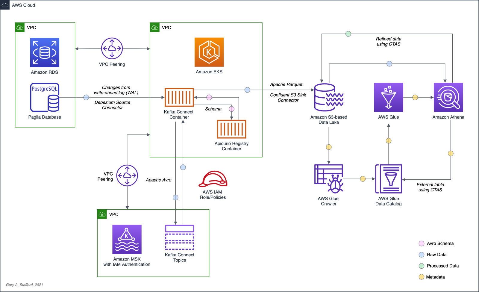
In the following post, we will explore one possible architecture for building a near real-time transactional data lake on AWS. The data lake will be built using a combination of open source software (OSS) and fully-managed AWS services. Red Hat’s Debezium, Apache Kafka, and Kafka Connect will be used for change data capture (CDC). In addition, Apache Spark, Apache Hudi, and Hudi’s DeltaStreamer will be used to manage the data lake. To complete our architecture, we will use several fully-managed AWS services, including Amazon RDS, Amazon MKS, Amazon EKS, AWS Glue, and Amazon EMR.

Source Code
The source code, configuration files, and a list of commands shown in this post are open-sourced and available on GitHub.
Kafka
According to the Apache Kafka documentation, “Apache Kafka is an open-source distributed event streaming platform used by thousands of companies for high-performance data pipelines, streaming analytics, data integration, and mission-critical applications.” For this post, we will use Apache Kafka as the core of our change data capture (CDC) process. According to Wikipedia, “change data capture (CDC) is a set of software design patterns used to determine and track the data that has changed so that action can be taken using the changed data. CDC is an approach to data integration that is based on the identification, capture, and delivery of the changes made to enterprise data sources.” We will discuss CDC in greater detail later in the post.
There are several options for Apache Kafka on AWS. We will use AWS’s fully-managed Amazon Managed Streaming for Apache Kafka (Amazon MSK) service. Alternatively, you could choose industry-leading SaaS providers, such as Confluent, Aiven, Redpanda, or Instaclustr. Lastly, you could choose to self-manage Apache Kafka on Amazon Elastic Compute Cloud (Amazon EC2) or Amazon Elastic Kubernetes Service (Amazon EKS).
Kafka Connect
According to the Apache Kafka documentation, “Kafka Connect is a tool for scalably and reliably streaming data between Apache Kafka and other systems. It makes it simple to quickly define connectors that move large collections of data into and out of Kafka. Kafka Connect can ingest entire databases or collect metrics from all your application servers into Kafka topics, making the data available for stream processing with low latency.”
There are multiple options for Kafka Connect on AWS. You can use AWS’s fully-managed, serverless Amazon MSK Connect. Alternatively, you could choose a SaaS provider or self-manage Kafka Connect yourself on Amazon Elastic Compute Cloud (Amazon EC2) or Amazon Elastic Kubernetes Service (Amazon EKS). I am not a huge fan of Amazon MSK Connect during development. In my opinion, iterating on the configuration for a new source and sink connector, especially with transforms and external registry dependencies, can be painfully slow and time-consuming with MSK Connect. I find it much faster to develop and fine-tune my sink and source connectors using a self-managed version of Kafka Connect. For Production workloads, you can easily port the configuration from the native Kafka Connect connector to MSK Connect. I am using a self-managed version of Kafka Connect for this post, running in Amazon EKS.

Debezium
According to the Debezium documentation, “Debezium is an open source distributed platform for change data capture. Start it up, point it at your databases, and your apps can start responding to all of the inserts, updates, and deletes that other apps commit to your databases.” Regarding Kafka Connect, according to the Debezium documentation, “Debezium is built on top of Apache Kafka and provides a set of Kafka Connect compatible connectors. Each of the connectors works with a specific database management system (DBMS). Connectors record the history of data changes in the DBMS by detecting changes as they occur and streaming a record of each change event to a Kafka topic. Consuming applications can then read the resulting event records from the Kafka topic.”
Source Connectors
We will use Kafka Connect along with three Debezium connectors, MySQL, PostgreSQL, and SQL Server, to connect to three corresponding Amazon Relational Database Service (RDS) databases and perform CDC. Changes from the three databases will be represented as messages in separate Kafka topics. In Kafka Connect terminology, these are referred to as Source Connectors. According to Confluent.io, a leader in the Kafka community, “source connectors ingest entire databases and stream table updates to Kafka topics.”
Sink Connector
We will stream the data from the Kafka topics into Amazon S3 using a sink connector. Again, according to Confluent.io, “sink connectors deliver data from Kafka topics to secondary indexes, such as Elasticsearch, or batch systems such as Hadoop for offline analysis.” We will use Confluent’s Amazon S3 Sink Connector for Confluent Platform. We can use Confluent’s sink connector without depending on the entire Confluent platform.
There is also an option to use the Hudi Sink Connector for Kafka, which promises to greatly simplify the processes described in this post. However, the RFC for this Hudi feature appears to be stalled. Last updated in August 2021, the RFC is still in the initial “Under Discussion” phase. Therefore, I would not recommend the connectors use in Production until it is GA (General Availability) and gains broader community support.
Securing Database Credentials
Whether using Amazon MSK Connect or self-managed Kafka Connect, you should ensure your database, Kafka, and schema registry credentials, and other sensitive configuration values are secured. Both MSK Connect and self-managed Kafka Connect can integrate with configuration providers that implement the ConfigProvider class interface, such as AWS Secrets Manager, HashiCorp Vault, Microsoft Azure Key Vault, and Google Cloud Secrets Manager.
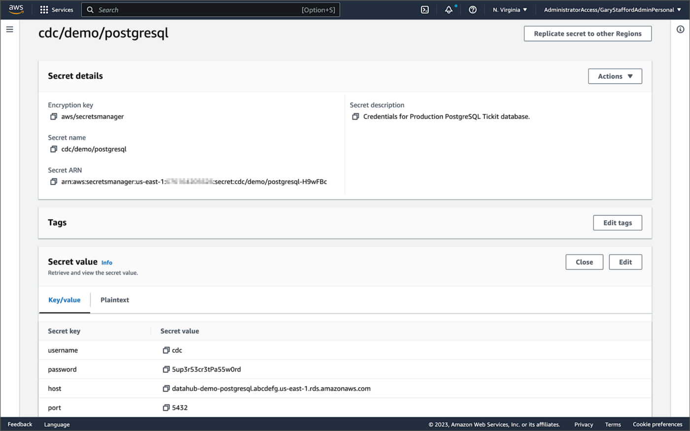
For self-managed Kafka Connect, I prefer Jeremy Custenborder’s kafka-config-provider-aws plugin. This plugin provides integration with AWS Secrets Manager. A complete list of Jeremy’s providers can be found on GitHub. Below is a snippet of the Secrets Manager configuration from the connect-distributed.properties files, which is read by Apache Kafka Connect at startup.
https://garystafford.medium.com/media/db6ff589c946fcd014546c56d0255fe5
Apache Avro
The message in the Kafka topic and corresponding objects in Amazon S3 will be stored in Apache Avro format by the CDC process. The Apache Avro documentation states, “Apache Avro is the leading serialization format for record data, and the first choice for streaming data pipelines.” Avro provides rich data structures and a compact, fast, binary data format.
Again, according to the Apache Avro documentation, “Avro relies on schemas. When Avro data is read, the schema used when writing it is always present. This permits each datum to be written with no per-value overheads, making serialization both fast and small. This also facilitates use with dynamic, scripting languages, since data, together with its schema, is fully self-describing.” When Avro data is stored in a file, its schema can be stored with it so any program may process files later.
Alternatively, the schema can be stored separately in a schema registry. According to Apicurio Registry, “in the messaging and event streaming world, data that are published to topics and queues often must be serialized or validated using a Schema (e.g. Apache Avro, JSON Schema, or Google protocol buffers). Schemas can be packaged in each application, but it is often a better architectural pattern to instead register them in an external system [schema registry] and then referenced from each application.”
Schema Registry
Several leading open-source and commercial schema registries exist, including Confluent Schema Registry, AWS Glue Schema Registry, and Red Hat’s open-source Apicurio Registry. In this post, we use a self-managed version of Apicurio Registry running on Amazon EKS. You can relatively easily substitute AWS Glue Schema Registry if you prefer a fully-managed AWS service.
Apicurio Registry
According to the documentation, Apicurio Registry supports adding, removing, and updating OpenAPI, AsyncAPI, GraphQL, Apache Avro, Google protocol buffers, JSON Schema, Kafka Connect schema, WSDL, and XML Schema (XSD) artifact types. Furthermore, content evolution can be controlled by enabling content rules, including validity and compatibility. Lastly, the registry can be configured to store data in various backend storage systems depending on the use case, including Kafka (e.g., Amazon MSK), PostgreSQL (e.g., Amazon RDS), and Infinispan (embedded).
Data Lake Table Formats
Three leading open-source, transactional data lake storage frameworks enable building data lake and data lakehouse architectures: Apache Iceberg, Linux Foundation Delta Lake, and Apache Hudi. They offer comparable features, such as ACID-compliant transactional guarantees, time travel, rollback, and schema evolution. Using any of these three data lake table formats will allow us to store and perform analytics on the latest version of the data in the data lake originating from the three Amazon RDS databases.
Apache Hudi
According to the Apache Hudi documentation, “Apache Hudi is a transactional data lake platform that brings database and data warehouse capabilities to the data lake.” The specifics of how the data is laid out as files in your data lake depends on the Hudi table type you choose, either Copy on Write (CoW) or Merge On Read (MoR).
Like Apache Iceberg and Delta Lake, Apache Hudi is partially supported by AWS’s Analytics services, including AWS Glue, Amazon EMR, Amazon Athena, Amazon Redshift Spectrum, and AWS Lake Formation. In general, CoW has broader support on AWS than MoR. It is important to understand the limitations of Apache Hudi with each AWS analytics service before choosing a table format.
If you are looking for a fully-managed Cloud data lake service built on Hudi, I recommend Onehouse. Born from the roots of Apache Hudi and founded by its original creator, Vinoth Chandar (PMC chair of the Apache Hudi project), the Onehouse product and its services leverage OSS Hudi to offer a data lake platform similar to what companies like Uber have built.
Hudi DeltaStreamer
Hudi also offers DeltaStreamer (aka HoodieDeltaStreamer) for streaming ingestion of CDC data. DeltaStreamer can be run once or continuously, using Apache Spark, similar to an Apache Spark Structured Streaming job, to capture changes to the raw CDC data and write that data to a different part of our data lake.
DeltaStreamer also works with Amazon S3 Event Notifications instead of running continuously. According to DeltaStreamer’s documentation, Amazon S3 object storage provides an event notification service to post notifications when certain events happen in your S3 bucket. AWS will put these events in Amazon Simple Queue Service (Amazon SQS). Apache Hudi provides an S3EventsSource that can read from Amazon SQS to trigger and process new or changed data as soon as it is available on Amazon S3.
Sample Data for the Data Lake
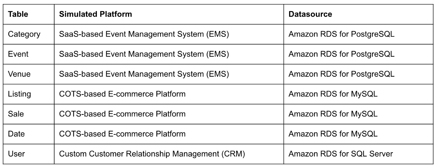
The data used in this post is from the TICKIT sample database. The TICKIT database represents the backend data store for a platform that brings buyers and sellers of tickets to entertainment events together. It was initially designed to demonstrate Amazon Redshift. The TICKIT database is a small database with approximately 425K rows of data across seven tables: Category, Event, Venue, User, Listing, Sale, and Date.
A data lake most often contains data from multiple sources, each with different storage formats, protocols, and connection methods. To simulate these data sources, I have separated the TICKIT database tables to represent three typical enterprise systems, including a commercial off-the-shelf (COTS) E-commerce platform, a custom Customer Relationship Management (CRM) platform, and a SaaS-based Event Management System (EMS). Each simulated system uses a different Amazon RDS database engine, including MySQL, PostgreSQL, and SQL Server.
Enabling CDC for Amazon RDS
To use Debezium for CDC with Amazon RDS databases, minor changes to the default database configuration for each database engine are required.
CDC for PostgreSQL
Debezium has detailed instructions regarding configuring CDC for Amazon RDS for PostgreSQL. Database parameters specify how the database is configured. According to the Debezium documentation, for PostgreSQL, set the instance parameter rds.logical_replication to 1 and verify that the wal_level parameter is set to logical. It is automatically changed when the rds.logical_replication parameter is set to 1. This parameter is adjusted using an Amazon RDS custom parameter group. According to the AWS documentation, “with Amazon RDS, you manage database configuration by associating your DB instances and Multi-AZ DB clusters with parameter groups. Amazon RDS defines parameter groups with default settings. You can also define your own parameter groups with customized settings.”

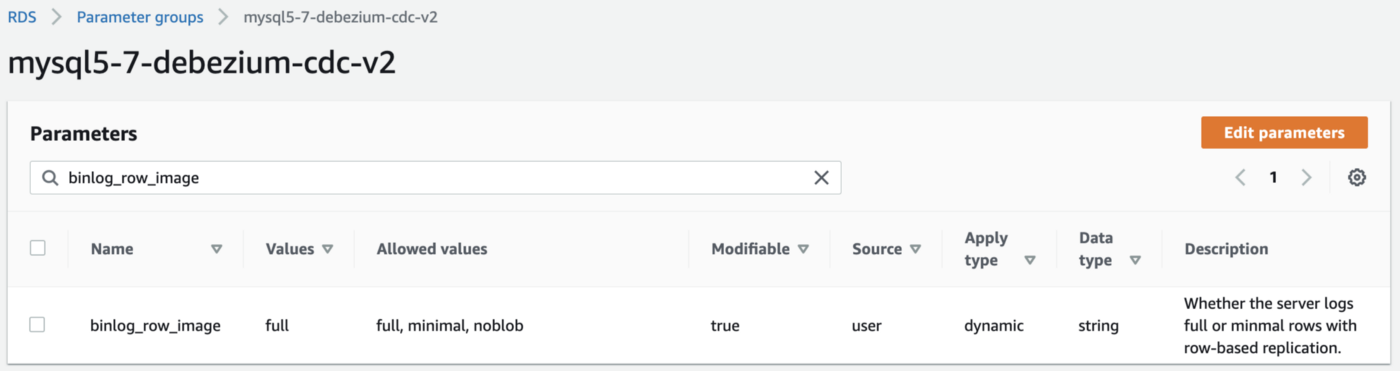
CDC for MySQL
Similarly, Debezium has detailed instructions regarding configuring CDC for MySQL. Like PostgreSQL, MySQL requires a custom DB parameter group.


CDC for SQL Server
Lastly, Debezium has detailed instructions for configuring CDC with Microsoft SQL Server. Enabling CDC requires enabling CDC on the SQL Server database and table(s) and creating a new filegroup and associated file. Debezium recommends locating change tables in a different filegroup than you use for source tables. CDC is only supported with Microsoft SQL Server Standard Edition and higher; Express and Web Editions are not supported.
Kafka Connect Source Connectors
There is a Kafka Connect source connector for each of the three Amazon RDS databases, all of which use Debezium. CDC is performed, moving changes from the three databases into separate Kafka topics in Apache Avro format using the source connectors. The connector configuration is nearly identical whether you are using Amazon MSK Connect or a self-managed version of Kafka Connect.
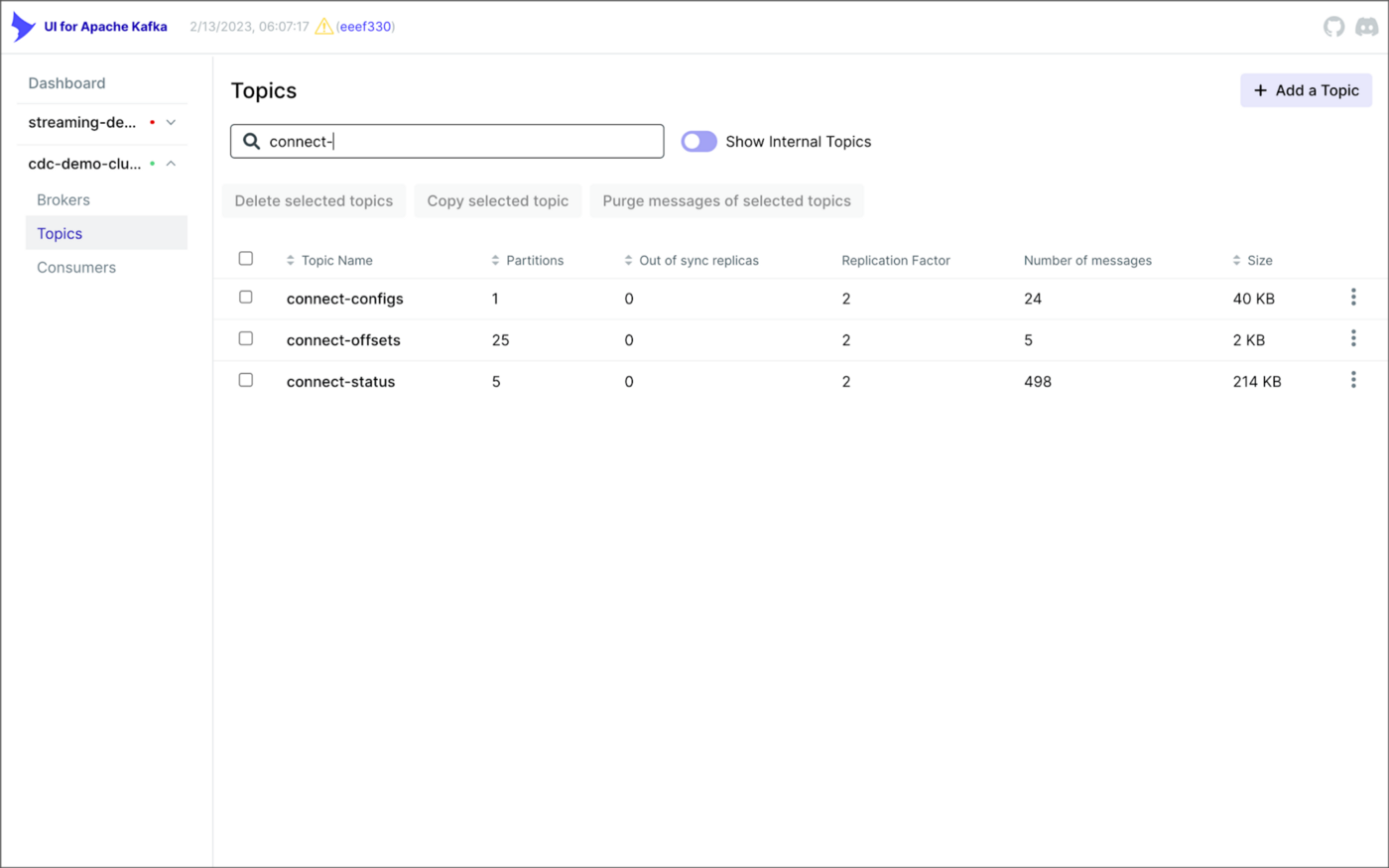
As shown above, I am using the UI for Apache Kafka by Provectus, self-managed on Amazon EKS, in this post.
PostgreSQL Source Connector
The source_connector_postgres_kafka_avro_tickit source connector captures all changes to the three tables in the Amazon RDS for PostgreSQL ticket database’s ems schema: category, event, and venue. These changes are written to three corresponding Kafka topics as Avro-format messages: tickit.ems.category, tickit.ems.event, and tickit.ems.venue. The messages are transformed by the connector using Debezium’s unwrap transform. Schemas for the messages are written to Apicurio Registry.
MySQL Source Connector
The source_connector_mysql_kafka_avro_tickit source connector captures all changes to the three tables in the Amazon RDS for PostgreSQL ecomm database: date, listing, and sale. These changes are written to three corresponding Kafka topics as Avro-format messages: tickit.ecomm.date, tickit.ecomm.listing, and tickit.ecomm.sale.
SQL Server Source Connector
Lastly, the source_connector_mssql_kafka_avro_tickit source connector captures all changes to the single user table in the Amazon RDS for SQL Server ticket database’s crm schema. These changes are written to a corresponding Kafka topic as Avro-format messages: tickit.crm.user.
If using a self-managed version of Kafka Connect, we can deploy, manage, and monitor the source and sink connectors using Kafka Connect’s RESTful API (Connect API).

Once the three source connectors are running, we should see seven new Kafka topics corresponding to the seven TICKIT database tables from the three Amazon RDS database sources. There will be approximately 425K messages consuming 147 MB of space in Avro’s binary format.
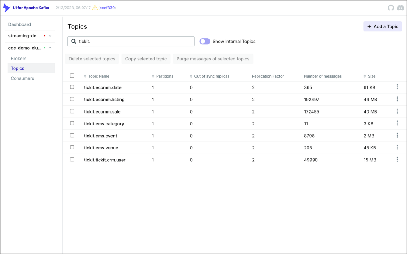
Avro’s binary format and the use of a separate schema ensure the messages consume minimal Kafka storage space. For example, the average message Value (payload) size in the tickit.ecomm.sale topic is a minuscule 98 Bytes. Resource management is critical when you are dealing with hundreds of millions or often billions of daily Kafka messages as a result of the CDC process.

From within the Apicurio Registry UI, we should now see Value schema artifacts for each of the seven Kafka topics.
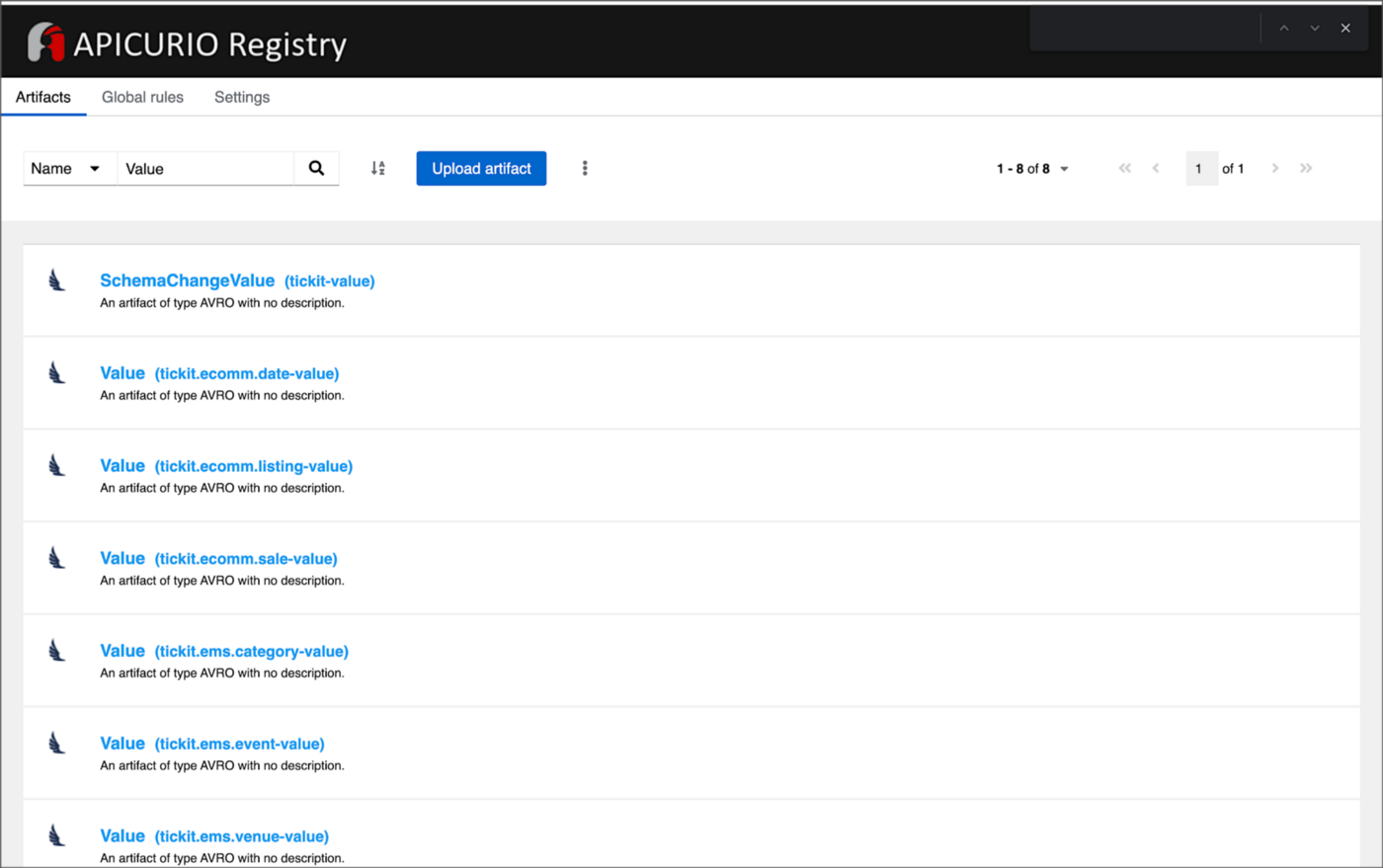
Also from within the Apicurio Registry UI, we can examine details of individual Value schema artifacts.

Kafka Connect Sink Connector
In addition to the three source connectors, there is a single Kafka Connect sink connector, sink_connector_kafka_s3_avro_tickit. The sink connector copies messages from the seven Kafka topics, all prefixed with tickit, to the Bronze area of our Amazon S3-based data lake.

The connector uses Confluent’s S3 Sink Connector (S3SinkConnector). Like Kafka, the connector writes all changes to Amazon S3 in Apache Avro format, with the schemas already stored in Apicurio Registry.
Once the sink connector and the three source connectors are running with Kafka Connect, we should see a series of seven subdirectories within the Bronze area of the data lake.

Confluent offers a choice of data partitioning strategies. The sink connector we have deployed uses the Daily Partitioner. According to the documentation, the io.confluent.connect.storage.partitioner.DailyPartitioner is equivalent to the TimeBasedPartitioner with path.format='year'=YYYY/'month'=MM/'day'=dd and partition.duration.ms=86400000 (one day for one S3 object in each daily directory). Below is an example of Avro files (S3 objects) containing changes to the sale table. The objects are partitioned by the year, month, and day they were written to the S3 bucket.

Message Transformation
Previously, while discussing the Kafka Connect source connectors, I mentioned that the connector transforms the messages using the unwrap transform. By default, the changes picked up by Debezium during the CDC process contain several additional Debezium-related fields of data. An example of an untransformed message generated by Debezium from the PostgreSQL sale table is shown below.
When the PostgreSQL connector first connects to a particular PostgreSQL database, it starts by performing a consistent snapshot of each database schema. All existing records are captured. Unlike an UPDATE ("op" : "u") or a DELETE ("op" : "d"), these initial snapshot messages, like the one shown below, represent a READ operation ("op" : "r"). As a result, there is no before data only after.
According to Debezium’s documentation, “Debezium provides a single message transformation [SMT] that crosses the bridge between the complex and simple formats, the UnwrapFromEnvelope SMT.” Below, we see the results of Debezium’s unwrap transform of the same message. The unwrap transform flattens the nested JSON structure of the original message, adds the __deleted field, and includes fields based on the list included in the source connector’s configuration. These fields are prefixed with a double underscore (e.g., __table).
In the next section, we examine Apache Hudi will manage the data lake. An example of the same message, managed with Hudi, is shown below. Note the five additional Hudi data fields, prefixed with _hoodie_.
Apache Hudi
With database changes flowing into the Bronze area of our data lake, we are ready to use Apache Hudi to provide data lake capabilities such as ACID transactional guarantees, time travel, rollback, and schema evolution. Using Hudi allows us to store and perform analytics on a specific time-bound version of the data in the data lake. Without Hudi, a query for a single row of data could return multiple results, such as an initial CREATE record, multiple UPDATE records, and a DELETE record.
DeltaStreamer
Using Hudi’s DeltaStreamer, we will continuously stream changes from the Bronze area of the data lake to a Silver area, which Hudi manages. We will run DeltaStreamer continuously, similar to an Apache Spark Structured Streaming job, using Apache Spark on Amazon EMR. Running DeltaStreamer requires using a spark-submit command that references a series of configuration files. There is a common base set of configuration items and a group of configuration items specific to each database table. Below, we see the base configuration, base.properties.
The base configuration is referenced by each of the table-specific configuration files. For example, below, we see the tickit.ecomm.sale.properties configuration file for DeltaStreamer.
To run DeltaStreamer, you can submit an EMR Step or use EMR’s master node to run a spark-submit command on the cluster. Below, we see an example of the DeltaStreamer spark-submit command using the Merge on Read (MoR) Hudi table type.
Next, we see the same example of the DeltaStreamer spark-submit command using the Copy on Write (CoW) Hudi table type.
For this post’s demonstration, we will run a single-table DeltaStreamer Spark job, with one process for each table using CoW. Alternately, Hudi offers HoodieMultiTableDeltaStreamer, a wrapper on top of HoodieDeltaStreamer, which enables the ingestion of multiple tables at a single time into Hudi datasets. Currently, HoodieMultiTableDeltaStreamer only supports sequential processing of tables to be ingested and COPY_ON_WRITE storage type.
Below, we see an example of three DeltaStreamer Spark jobs running continuously for the date, listing, and sale tables.

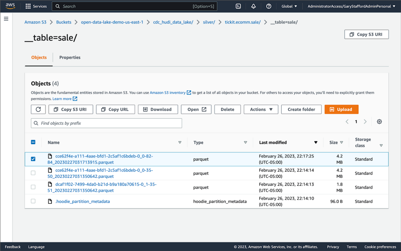
Once DeltaStreamer is up and running, we should see a series of subdirectories within the Silver area of the data lake, all managed by Apache Hudi.
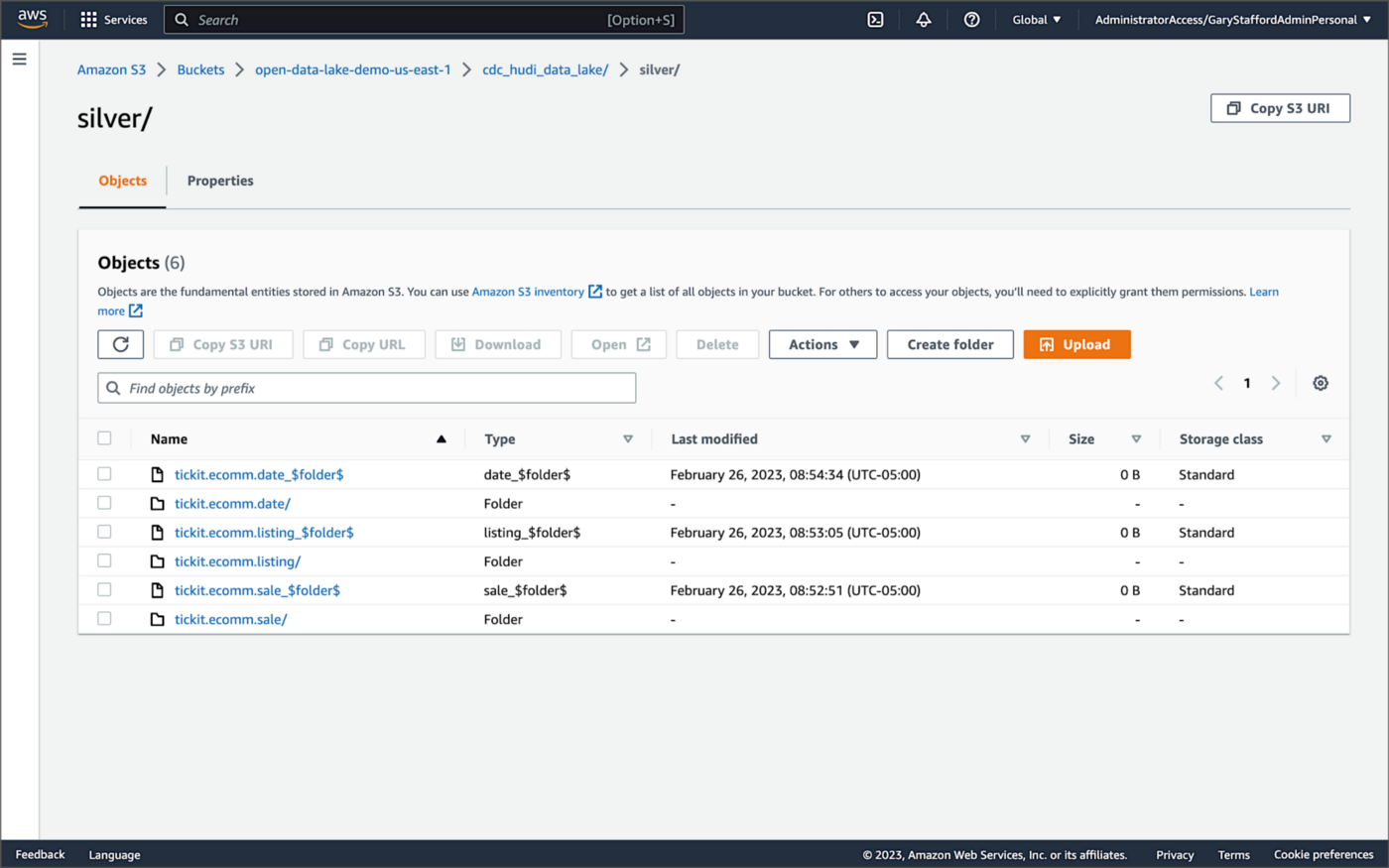
Within each subdirectory, partitioned by the table name, is a series of Apache Parquet files, along with other Apache Hudi-specific files. The specific folder structure and files depend on MoR or Cow.

AWS Glue Data Catalog
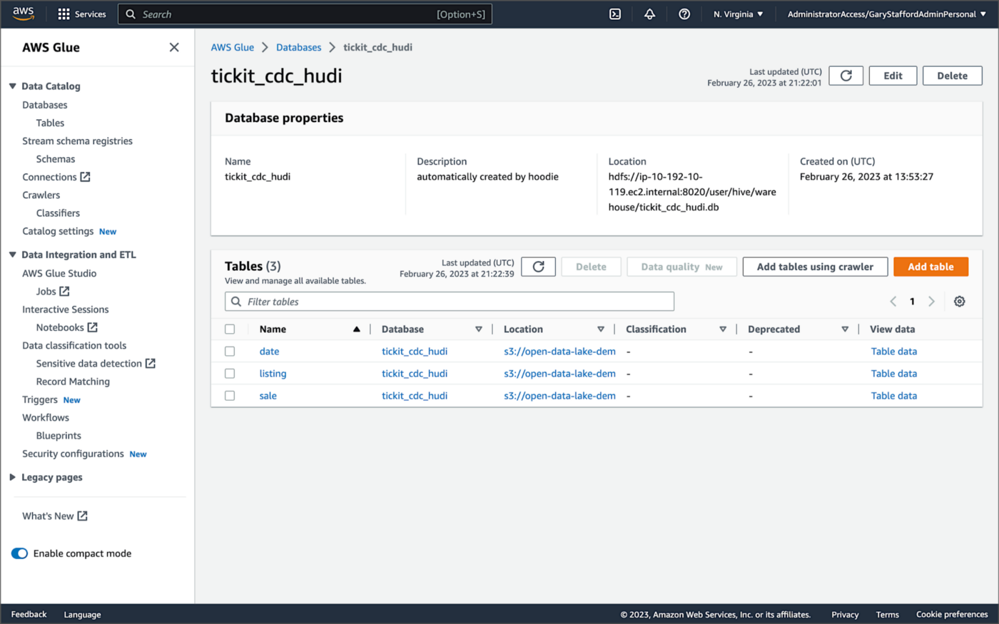
For this post, we are using an AWS Glue Data Catalog, an Apache Hive-compatible metastore, to persist technical metadata stored in the Silver area of the data lake, managed by Apache Hudi. The AWS Glue Data Catalog database, tickit_cdc_hudi, will be automatically created the first time DeltaStreamer runs.
Using DeltaStreamer with the table type of MERGE_ON_READ, there would be two tables in the AWS Glue Data Catalog database for each original table. According to Amazon’s EMR documentation, “Merge on Read (MoR) — Data is stored using a combination of columnar (Parquet) and row-based (Avro) formats. Updates are logged to row-based delta files and are compacted as needed to create new versions of the columnar files.” Hudi creates two tables in the Hive metastore for MoR, a table with the name that you specified, which is a read-optimized view (appended with _ro), and a table with the same name appended with _rt, which is a real-time view. You can query both tables.
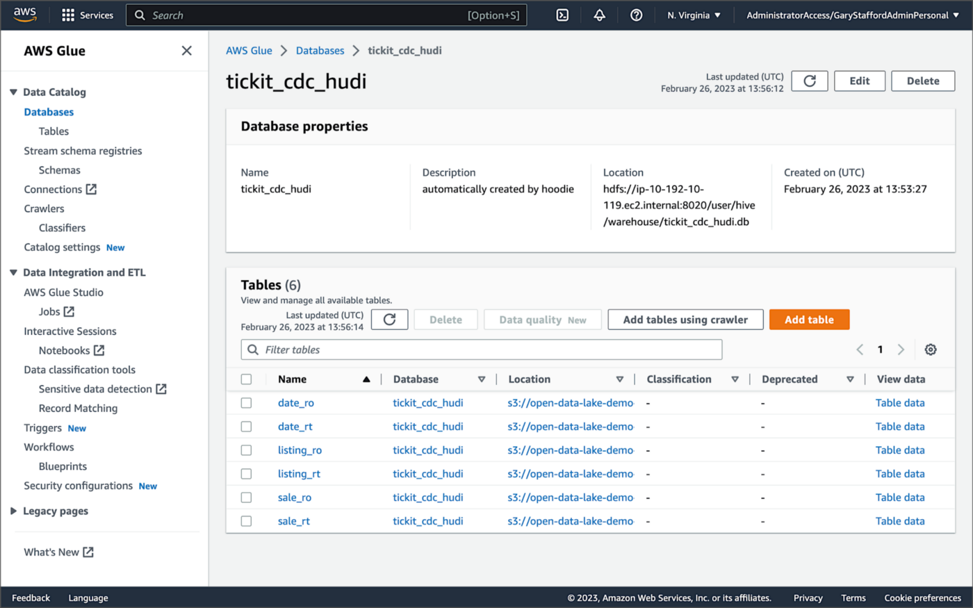
According to Amazon’s EMR documentation, “Copy on Write (CoW) — Data is stored in a columnar format (Parquet), and each update creates a new version of files during a write. CoW is the default storage type.” Using COPY_ON_WRITE with DeltaStreamer, there is only a single Hudi table in the AWS Glue Data Catalog database for each corresponding database table.
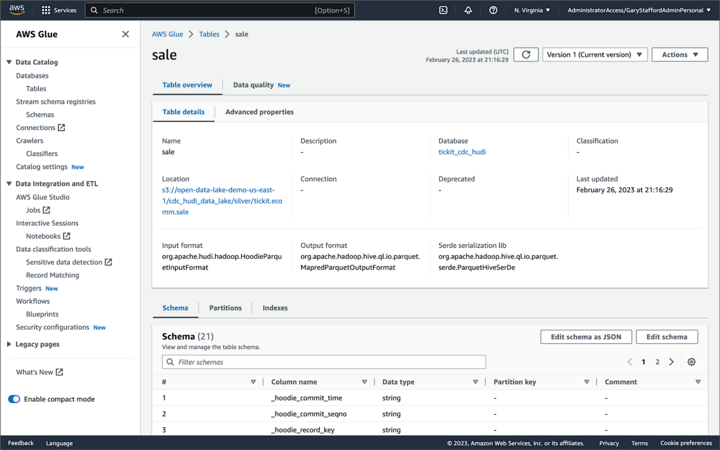
Examining an individual table in the AWS Glue Data Catalog database, we can see details like the table schema, location of underlying data in S3, input/output formats, Serde serialization library, and table partitions.
Database Changes and Data Lake
We are using Kafka Connect, Apache Hudi, and Hudi’s DeltaStreamer to maintain data parity between our databases and the data lake. Let’s look at an example of how a simple data change is propagated from a database to Kafka, then to the Bronze area of the data lake, and finally to the Hudi-managed Silver area of the data lake, written using the CoW table format.
First, we will make a simple update to a single record in the MySQL database’s sale table with the salesid = 200.
Almost immediately, we can see the change picked up by the Kafka Connect Debezium MySQL source connector.

Almost immediately, in the Bronze area of the data lake, we can see we have a new Avro-formatted file (S3 object) containing the updated record in the partitioned sale subdirectory.

If we examine the new object in the Bronze area of the data lake, we will see a row representing the updated record with the salesid = 200. Note how the operation is now an UPDATE versus a READ ("op" : "u").
Next, in the corresponding Silver area of the data lake, managed by Hudi, we should also see a new Parquet file that contains a record of the change. In this example, the file was written approximately 26 seconds after the original change to the database. This is the end-to-end time from database change to when the updated data is queryable in the data lake.
Similarly, if we examine the new object in the Silver area of the data lake, we will see a row representing the updated record with the salesid = 200. The record was committed approximately 15 seconds after the original database change.
Querying Hudi Tables with Amazon EMR
Using an EMR Notebook, we can query the updated database record stored in Amazon S3 using Hudi’s CoW table format. First, running a simple Spark SQL query for the record with salesid = 200, returns the latest record, reflecting the changes as indicated by the UPDATE operation value (u) and the _hoodie_commit_time = 2023-02-27 03:17:13.915 UTC.

Hudi Time Travel Query
We can also run a Hudi Time Travel Query, with an as.of.instance set to some arbitrary point in the future. Again, the latest record is returned, reflecting the changes as indicated by the UPDATE operation value (u) and the _hoodie_commit_time = 2023-02-27 03:17:13.915 UTC.

We can run the same Hudi Time Travel Query with an as.of.instance set to on or after the original records were written by DeltaStreamer (_hoodie_commit_time = 2023-02-27 03:13:50.642), but some arbitrary time before the updated record was written (_hoodie_commit_time = 2023-02-27 03:17:13.915). This time, the original record is returned as indicated by the READ operation value (r) and the _hoodie_commit_time = 2023-02-27 03:13:50.642. This is one of the strengths of Apache Hudi, the ability to query data in the present or at any point in the past.

Hudi Point in Time Query
We can also run a Hudi Point in Time Query, with a time range set from the beginning of time until some arbitrary point in the future. Again, the latest record is returned, reflecting the changes as indicated by the UPDATE operation value (u) and the _hoodie_commit_time = 2023-02-27 03:17:13.915.

We can run the same Hudi Point in Time Query but change the time range to two arbitrary time values, both before the updated record was written (_hoodie_commit_time = 2023-02-26 22:39:07.203). This time, the original record is returned as indicated by the READ operation value (r) and the _hoodie_commit_time of 2023-02-27 03:13:50.642. Again, this is one of the strengths of Apache Hudi, the ability to query data in the present or at any point in the past.

Querying Hudi Tables with Amazon Athena
We can also use Amazon Athena and run a SQL query against the AWS Glue Data Catalog database’s sale table to view the updated database record stored in Amazon S3 using Hudi’s CoW table format. The operation (op) column’s value now indicates an UPDATE (u).

How are Deletes Handled?
In this post’s architecture, deleted database records are signified with an operation ("op") field value of "d" for a DELETE and a __deleted field value of true.
https://itnext.io/media/f7c4ad62dcd45543fdf63834814a5aab
Back to our previous Jupyter notebook example, when rerunning the Spark SQL query, the latest record is returned, reflecting the changes as indicated by the DELETE operation value (d) and the _hoodie_commit_time = 2023-02-27 03:52:13.689.

Alternatively, we could use an additional Spark SQL filter statement to prevent deleted records from being returned (e.g., df.__op != "d").

Since we only did what is referred to as a soft delete in Hudi terminology, we can run a time travel query with an as.of.instance set to some arbitrary time before the deleted record was written (_hoodie_commit_time = 2023-02-27 03:52:13.689). This time, the original record is returned as indicated by the READ operation value (r) and the _hoodie_commit_time = 2023-02-27 03:13:50.642. We could also use a later as.of.instance to return the version of the record reflecting the the UPDATE operation value (u). This also applies to other query types such as point-in-time queries.

Conclusion
In this post, we learned how to build a near real-time transactional data lake on AWS using one possible architecture. The data lake was built using a combination of open source software (OSS) and fully-managed AWS services. Red Hat’s Debezium, Apache Kafka, and Kafka Connect were used for change data capture (CDC). In addition, Apache Spark, Apache Hudi, and Hudi’s DeltaStreamer were used to manage the data lake. To complete our architecture, we used several fully-managed AWS services, including Amazon RDS, Amazon MKS, Amazon EKS, AWS Glue, and Amazon EMR.
This blog represents my own viewpoints and not of my employer, Amazon Web Services (AWS). All product names, logos, and brands are the property of their respective owners.
Video Demonstration: Building Open Data Lakes on AWS with Debezium and Apache Hudi
Posted by Gary A. Stafford in Software Development on October 31, 2021
Build an open-source data lake on AWS using a combination of Debezium, Apache Kafka, Apache Hudi, Apache Spark, and Apache Hive
Introduction
In the following recorded demonstration, we will build a simple open data lake on AWS using a combination of open-source software (OSS), including Red Hat’s Debezium, Apache Kafka, and Kafka Connect for change data capture (CDC), and Apache Hive, Apache Spark, Apache Hudi, and Hudi’s DeltaStreamer for managing our data lake. We will use fully-managed AWS services to host the open data lake components, including Amazon RDS, Amazon MKS, Amazon EKS, and EMR.

Demonstration
Source Code
All source code for this post and the previous posts in this series are open-sourced and located on GitHub. The following files are used in the demonstration:
- MoMA data: Uncompress files and import pipe-delimited data to PostgreSQL;
base.properties: Base Hudi DeltaStreamer properties;deltastreamer_artists_file_based_schema.properties: Demo-specific Hudi DeltaStreamer properties for MoMA Artists;deltastreamer_artworks_file_based_schema.properties: Demo-specific Hudi DeltaStreamer properties for MoMA Artworks;source_connector_moma_postgres_kafka.json: Kafka Connect Source Connector (PostgreSQL to Kafka);sink_connector_moma_kafka_s3.json: Kafka Connect Sink Connector (Kafka to Amazon S3);moma_debezium_hudi_demo.ipynb: Jupyter PySpark Notebook;demonstration_notes.md: Commands used in the demonstration;
This blog represents my own viewpoints and not of my employer, Amazon Web Services (AWS). All product names, logos, and brands are the property of their respective owners.
Hydrating a Data Lake using Log-based Change Data Capture (CDC) with Debezium, Apicurio, and Kafka Connect on AWS
Posted by Gary A. Stafford in Analytics, AWS, Big Data, Cloud, Kubernetes on August 21, 2021
Import data from Amazon RDS into Amazon S3 using Amazon MSK, Apache Kafka Connect, Debezium, Apicurio Registry, and Amazon EKS
Introduction
In the last post, Hydrating a Data Lake using Query-based CDC with Apache Kafka Connect and Kubernetes on AWS, we utilized Kafka Connect to export data from an Amazon RDS for PostgreSQL relational database and import the data into a data lake built on Amazon Simple Storage Service (Amazon S3). The data imported into S3 was converted to Apache Parquet columnar storage file format, compressed, and partitioned for optimal analytics performance, all using Kafka Connect. To improve data freshness, as data was added or updated in the PostgreSQL database, Kafka Connect automatically detected those changes and streamed them into the data lake using query-based Change Data Capture (CDC).
This follow-up post will examine log-based CDC as a marked improvement over query-based CDC to continuously stream changes from the PostgreSQL database to the data lake. We will perform log-based CDC using Debezium’s Kafka Connect Source Connector for PostgreSQL rather than Confluent’s Kafka Connect JDBC Source connector, which was used in the previous post for query-based CDC. We will store messages as Apache Avro in Kafka running on Amazon Managed Streaming for Apache Kafka (Amazon MSK). Avro message schemas will be stored in Apicurio Registry. The schema registry will run alongside Kafka Connect on Amazon Elastic Kubernetes Service (Amazon EKS).
Change Data Capture
According to Gunnar Morling, Principal Software Engineer at Red Hat, who works on the Debezium and Hibernate projects, and well-known industry speaker, there are two types of Change Data Capture — Query-based and Log-based CDC. Gunnar detailed the differences between the two types of CDC in his talk at the Joker International Java Conference in February 2021, Change data capture pipelines with Debezium and Kafka Streams.

You can find another excellent explanation of CDC in the recent post by Lewis Gavin of Rockset, Change Data Capture: What It Is and How to Use It.
Query-based vs. Log-based CDC
To demonstrate the high-level differences between query-based and log-based CDC, let’s examine the results of a simple SQL UPDATE statement captured with both CDC methods.
UPDATE public.address
SET address2 = 'Apartment #1234'
WHERE address_id = 105;
Here is how that change is represented as a JSON message payload using the query-based CDC method described in the previous post.
{
  "address_id": 105,
  "address": "733 Mandaluyong Place",
  "address2": "Apartment #1234",
  "district": "Asir",
  "city_id": 2,
  "postal_code": "77459",
  "phone": "196568435814",
  "last_update": "2021-08-13T00:43:38.508Z"
}
Here is how the same change is represented as a JSON message payload using log-based CDC with Debezium. Note the metadata-rich structure of the log-based CDC message as compared to the query-based message.
{
  "after": {
    "address": "733 Mandaluyong Place",
    "address2": "Apartment #1234",
    "phone": "196568435814",
    "district": "Asir",
    "last_update": "2021-08-13T00:43:38.508453Z",
    "address_id": 105,
    "postal_code": "77459",
    "city_id": 2
  },
  "source": {
    "schema": "public",
    "sequence": "[\"1090317720392\",\"1090317720392\"]",
    "xmin": null,
    "connector": "postgresql",
    "lsn": 1090317720624,
    "name": "pagila",
    "txId": 16973,
    "version": "1.6.1.Final",
    "ts_ms": 1628815418508,
    "snapshot": "false",
    "db": "pagila",
    "table": "address"
  },
  "op": "u",
  "ts_ms": 1628815418815
}
Avro and Schema Registry
Apache Avro is a compact, fast, binary data format, according to the documentation. Avro relies on schemas. When Avro data is read, the schema used when writing it is always present. This permits each datum to be written with no per-value overheads, making serialization both fast and small. This also facilitates use with dynamic scripting languages since data, together with its schema, is fully self-describing.
We can decouple the data from its schema by using schema registries like the Confluent Schema Registry or Apicurio Registry. According to Apicurio, in a messaging and event streaming architecture, data published to topics and queues must often be serialized or validated using a schema (e.g., Apache Avro, JSON Schema, or Google Protocol Buffers). Of course, schemas can be packaged in each application. Still, it is often a better architectural pattern to register schemas in an external system [schema registry] and then reference them from each application.
It is often a better architectural pattern to register schemas in an external system and then reference them from each application.
Using Debezium’s PostgreSQL source connector, we will store changes from the PostgreSQL database’s write-ahead log (WAL) as Avro in Kafka, running on Amazon MSK. The message’s schema will be stored separately in Apicurio Registry as opposed to with the message, thus reducing the size of the messages in Kafka and allowing for schema validation and schema evolution.

pagila.public.film schemaDebezium
Debezium, according to their website, continuously monitors your databases and lets any of your applications stream every row-level change in the same order they were committed to the database. Event streams can be used to purge caches, update search indexes, generate derived views and data, and keep other data sources in sync. Debezium is a set of distributed services that capture row-level changes in your databases. Debezium records all row-level changes committed to each database table in a transaction log. Then, each application reads the transaction logs they are interested in, and they see all of the events in the same order in which they occurred. Debezium is built on top of Apache Kafka and integrates with Kafka Connect.
The latest version of Debezium includes support for monitoring MySQL database servers, MongoDB replica sets or sharded clusters, PostgreSQL servers, and SQL Server databases. We will be using Debezium’s PostgreSQL connector to capture row-level changes in the Pagila PostgreSQL database. According to Debezium’s documentation, the first time it connects to a PostgreSQL server or cluster, the connector takes a consistent snapshot of all schemas. After that snapshot is complete, the connector continuously captures row-level changes that insert, update, and delete database content committed to the database. The connector generates data change event records and streams them to Kafka topics. For each table, the default behavior is that the connector streams all generated events to a separate Kafka topic for that table. Applications and services consume data change event records from that topic.
Prerequisites
Similar to the previous post, this post will focus on data movement, not how to deploy the required AWS resources. To follow along with the post, you will need the following resources already deployed and configured on AWS:
- Amazon RDS for PostgreSQL instance (data source);
- Amazon S3 bucket (data sink);
- Amazon MSK cluster;
- Amazon EKS cluster;
- Connectivity between the Amazon RDS instance and Amazon MSK cluster;
- Connectivity between the Amazon EKS cluster and Amazon MSK cluster;
- Ensure the Amazon MSK Configuration has
auto.create.topics.enable=true. This setting isfalseby default; - IAM Role associated with Kubernetes service account (known as IRSA) that will allow access from EKS to MSK and S3 (see details below);
As shown in the architectural diagram above, I am using three separate VPCs within the same AWS account and AWS Region, us-east-1, for Amazon RDS, Amazon EKS, and Amazon MSK. The three VPCs are connected using VPC Peering. Ensure you expose the correct ingress ports, and the corresponding CIDR ranges on your Amazon RDS, Amazon EKS, and Amazon MSK Security Groups. For additional security and cost savings, use a VPC endpoint to ensure private communications between Amazon EKS and Amazon S3.
Source Code
All source code for this post and the previous post, including the Kafka Connect and connector configuration files and the Helm charts, is open-sourced and located on GitHub.GitHub — garystafford/kafka-connect-msk-demo: For the post, Hydrating a Data Lake using Change Data…
For the post, Hydrating a Data Lake using Change Data Capture (CDC), Apache Kafka, and Kubernetes on AWS — GitHub …github.com
Authentication and Authorization
Amazon MSK provides multiple authentication and authorization methods to interact with the Apache Kafka APIs. For example, you can use IAM to authenticate clients and to allow or deny Apache Kafka actions. Alternatively, you can use TLS or SASL/SCRAM to authenticate clients and Apache Kafka ACLs to allow or deny actions. In my last post, I demonstrated the use of SASL/SCRAM and Kafka ACLs with Amazon MSK:Securely Decoupling Applications on Amazon EKS using Kafka with SASL/SCRAM
Securely decoupling Go-based microservices on Amazon EKS using Amazon MSK with IRSA, SASL/SCRAM, and data encryptionitnext.io
Any MSK authentication and authorization should work with Kafka Connect, assuming you correctly configure Amazon MSK, Amazon EKS, and Kafka Connect. For this post, we are using IAM Access Control. An IAM Role associated with a Kubernetes service account (known as IRSA) allows EKS to access MSK and S3 using IAM (see more details below).
Sample PostgreSQL Database
For this post, we will continue to use PostgreSQL’s Pagila database. The database contains simulated movie rental data. The dataset is fairly small, making it less ideal for ‘big data’ use cases but small enough to quickly install and minimize data storage and analytical query costs.

Before continuing, create a new database on the Amazon RDS PostgreSQL instance and populate it with the Pagila sample data. A few people have posted updated versions of this database with easy-to-install SQL scripts. Check out the Pagila scripts provided by Devrim Gündüz on GitHub and also by Robert Treat on GitHub.
Last Updated Trigger
Each table in the Pagila database has a last_update field. A simplistic way to detect changes in the Pagila database is to use the last_update field. This is a common technique to determine if and when changes were made to data using query-based CDC, as demonstrated in the previous post. As changes are made to records in these tables, an existing database function and a trigger to each table will ensure the last_update field is automatically updated to the current date and time. You can find further information on how the database function and triggers work with Kafka Connect in this post, kafka connect in action, part 3, by Dominick Lombardo.
CREATE OR REPLACE FUNCTION update_last_update_column()
    RETURNS TRIGGER AS
$$
BEGIN
    NEW.last_update = now();
    RETURN NEW;
END;
$$ language 'plpgsql';
CREATE TRIGGER update_last_update_column_address
    BEFORE UPDATE
    ON address
    FOR EACH ROW
EXECUTE PROCEDURE update_last_update_column();
Kafka Connect and Schema Registry
There are several options for deploying and managing Kafka Connect, the Kafka management APIs and command-line tools, and the Apicurio Registry. I prefer deploying a containerized solution to Kubernetes on Amazon EKS. Some popular containerized Kafka options include Strimzi, Confluent for Kubernetes (CFK), and Debezium. Another option is building your own Docker Image using the official Apache Kafka binaries. I chose to build my own Kafka Connect Docker Image using the latest Kafka binaries for this post. I then installed the necessary Confluent and Debezium connectors and their associated Java dependencies into the Kafka installation. Although not as efficient as using an off-the-shelf container, building your own image will teach you how Kafka, Kafka Connect, and Debezium work, in my opinion.
In regards to the schema registry, both Confluent and Apicurio offer containerized solutions. Apicurio has three versions of their registry, each with a different storage mechanism: in-memory, SQL, and Kafka. Since we already have an existing Amazon RDS PostgreSQL instance as part of the demonstration, I chose the Apicurio SQL-based registry Docker Image for this post, apicurio/apicurio-registry-sql:2.0.1.Final.
If you choose to use the same Kafka Connect and Apicurio solution I used in this post, a Helm Chart is included in the post’s GitHub repository, kafka-connect-msk-v2. The Helm chart will deploy a single Kubernetes pod to the kafka Namespace on Amazon EKS. The pod comprises both the Kafka Connect and Apicurio Registry containers. The deployment is intended for demonstration purposes and is not designed for use in Production.
apiVersion: v1
kind: Service
metadata:
  name: kafka-connect-msk
spec:
  type: NodePort
  selector:
    app: kafka-connect-msk
  ports:
    - port: 8080
---
apiVersion: apps/v1
kind: Deployment
metadata:
  name: kafka-connect-msk
  labels:
    app: kafka-connect-msk
    component: service
spec:
  replicas: 1
  strategy:
    type: Recreate
  selector:
    matchLabels:
      app: kafka-connect-msk
      component: service
  template:
    metadata:
      labels:
        app: kafka-connect-msk
        component: service
    spec:
      serviceAccountName: kafka-connect-msk-iam-serviceaccount
      containers:
        - image: garystafford/kafka-connect-msk:1.1.0
          name: kafka-connect-msk
          imagePullPolicy: IfNotPresent
        - image: apicurio/apicurio-registry-sql:2.0.1.Final
          name: apicurio-registry-mem
          imagePullPolicy: IfNotPresent
          env:
            - name: REGISTRY_DATASOURCE_URL
              value: jdbc:postgresql://your-pagila-database-url.us-east-1.rds.amazonaws.com:5432/apicurio-registry
            - name: REGISTRY_DATASOURCE_USERNAME
              value: apicurio_registry
            - name: REGISTRY_DATASOURCE_PASSWORD
              value: 1L0v3Kafka!
Before deploying the chart, create a new PostgreSQL database, user, and grants on your RDS instance for the Apicurio Registry to use for storage:
CREATE DATABASE "apicurio-registry";
CREATE USER apicurio_registry WITH PASSWORD '1L0v3KafKa!';

GRANT CONNECT, CREATE ON DATABASE "apicurio-registry" to apicurio_registry;
Update the Helm chart’s value.yaml file with the name of your Kubernetes Service Account associated with the Kafka Connect pod (serviceAccountName) and your RDS URL (registryDatasourceUrl). The IAM Policy attached to the IAM Role associated with the pod’s Service Account should provide sufficient access to Kafka running on the Amazon MSK cluster from EKS. The policy should also provide access to your S3 bucket, as detailed here by Confluent. Below is an example of an (overly broad) IAM Policy that would allow full access to any Kafka clusters running on Amazon MSK and to your S3 bucket from Kafka Connect running on Amazon EKS.
Once the variables are updated, use the following command to deploy the Helm chart:
helm install kafka-connect-msk-v2 ./kafka-connect-msk-v2 \
  --namespace $NAMESPACE --create-namespace
Confirm the chart was installed successfully by checking the pod’s status:
kubectl get pods -n kafka -l app=kafka-connect-msk

If you have any issues with either container while deploying, review the individual container’s logs:
export KAFKA_CONTAINER=$(
  kubectl get pods -n kafka -l app=kafka-connect-msk | \
    awk 'FNR == 2 {print $1}')
kubectl logs $KAFKA_CONTAINER -n kafka kafka-connect-msk
kubectl logs $KAFKA_CONTAINER -n kafka apicurio-registry-mem
Kafka Connect
Get a shell to the running Kafka Connect container using the kubectl exec command:
export KAFKA_CONTAINER=$(
  kubectl get pods -n kafka -l app=kafka-connect-msk | \
    awk 'FNR == 2 {print $1}')
kubectl exec -it $KAFKA_CONTAINER -n kafka -c kafka-connect-msk -- bash

Confirm Access to Registry from Kafka Connect
If the Helm Chart was deployed successfully, you should now observe 11 new tables in the public schema of the new apicurio-registry database. Below, we see the new database and tables, as shown in pgAdmin.

Confirm the registry is running and accessible from the Kafka Connect container by calling the registry’s system/info REST API endpoint:
curl -s http://localhost:8080/apis/registry/v2/system/info | jq

The Apicurio Registry’s Service targets TCP port 8080. The Service is exposed on the Kubernetes worker node’s external IP address at a static port, the NodePort. To get the NodePort of the service, use the following command:
kubectl describe services kafka-client-msk -n kafka
To access the Apicurio Registry’s web-based UI, add the NodePort to the Security Group of the EKS nodes with the source being your IP address, a /32 CIDR block.
To get the external IP address (EXTERNAL-IP) of any Amazon EKS worker nodes, use the following command:
kubectl get nodes -o wide
Use the <NodeIP>:<NodePort> combination to access the UI from your web browser, for example, http://54.237.41.128:30433. The registry will be empty at this point in the demonstration.

Configure Bootstrap Brokers
Before starting Kafka Connect, you will need to modify Kafka Connect’s configuration file. Kafka Connect is capable of running workers in standalone or distributed modes. Since we will be using Kafka Connect’s distributed mode, modify the config/connect-distributed.properties file. A complete sample of the configuration file I used in this post is shown below.
Kafka Connect and the schema registry will run on Amazon EKS, while Kafka and Apache ZooKeeper run on Amazon MSK. Update the bootstrap.servers property to reflect your own comma-delimited list of Amazon MSK Kafka Bootstrap Brokers. To get the list of the Bootstrap Brokers for your Amazon MSK cluster, use the AWS Management Console, or the following AWS CLI commands:
# get the msk cluster's arn
aws kafka list-clusters --query 'ClusterInfoList[*].ClusterArn'
# use msk arn to get the brokers
aws kafka get-bootstrap-brokers --cluster-arn your-msk-cluster-arn
# alternately, if you only have one cluster, then
aws kafka get-bootstrap-brokers --cluster-arn $(
  aws kafka list-clusters | jq -r '.ClusterInfoList[0].ClusterArn')
Update the config/connect-distributed.properties file.
# ***** CHANGE ME! *****
bootstrap.servers=b-1.your-cluster.123abc.c2.kafka.us-east-1.amazonaws.com:9098,b-2.your-cluster.123abc.c2.kafka.us-east-1.amazonaws.com:9098, b-3.your-cluster.123abc.c2.kafka.us-east-1.amazonaws.com:9098
group.id=connect-cluster
key.converter.schemas.enable=true
value.converter.schemas.enable=true
offset.storage.topic=connect-offsets
offset.storage.replication.factor=2
#offset.storage.partitions=25
config.storage.topic=connect-configs
config.storage.replication.factor=2
status.storage.topic=connect-status
status.storage.replication.factor=2
#status.storage.partitions=5
offset.flush.interval.ms=10000
plugin.path=/usr/local/share/kafka/plugins
# kafka connect auth using iam
ssl.truststore.location=/tmp/kafka.client.truststore.jks
security.protocol=SASL_SSL
sasl.mechanism=AWS_MSK_IAM
sasl.jaas.config=software.amazon.msk.auth.iam.IAMLoginModule required;
sasl.client.callback.handler.class=software.amazon.msk.auth.iam.IAMClientCallbackHandler
# kafka connect producer auth using iam
producer.ssl.truststore.location=/tmp/kafka.client.truststore.jks
producer.security.protocol=SASL_SSL
producer.sasl.mechanism=AWS_MSK_IAM
producer.sasl.jaas.config=software.amazon.msk.auth.iam.IAMLoginModule required;
producer.sasl.client.callback.handler.class=software.amazon.msk.auth.iam.IAMClientCallbackHandler
# kafka connect consumer auth using iam
consumer.ssl.truststore.location=/tmp/kafka.client.truststore.jks
consumer.security.protocol=SASL_SSL
consumer.sasl.mechanism=AWS_MSK_IAM
consumer.sasl.jaas.config=software.amazon.msk.auth.iam.IAMLoginModule required;
consumer.sasl.client.callback.handler.class=software.amazon.msk.auth.iam.IAMClientCallbackHandler
For convenience when executing Kafka commands, set the BBROKERS environment variable to the same comma-delimited list of Kafka Bootstrap Brokers, for example:
export BBROKERS="b-1.your-cluster.123abc.c2.kafka.us-east-1.amazonaws.com:9098,b-2.your-cluster.123abc.c2.kafka.us-east-1.amazonaws.com:9098, b-3.your-cluster.123abc.c2.kafka.us-east-1.amazonaws.com:9098"
Confirm Access to Amazon MSK from Kafka Connect
To confirm you have access to Kafka running on Amazon MSK, from the Kafka Connect container running on Amazon EKS, try listing the exiting Kafka topics:
bin/kafka-topics.sh --list \
  --bootstrap-server $BBROKERS \
  --command-config config/client-iam.properties
You can also try listing the existing Kafka consumer groups:
bin/kafka-consumer-groups.sh --list \
  --bootstrap-server $BBROKERS \
  --command-config config/client-iam.properties
If either of these fails, you likely have networking or security issues blocking access from Amazon EKS to Amazon MSK. Check your VPC Peering, Route Tables, IAM/IRSA, and Security Group ingress settings. Any one of these items can cause communications issues between the container and Kafka running on Amazon MSK.
Once configured, start Kafka Connect as a background process.
Kafka Connect
bin/connect-distributed.sh \
  config/connect-distributed.properties > /dev/null 2>&1 &
To confirm Kafka Connect starts properly, immediately tail the connect.log file. The log will capture any startup errors for troubleshooting.
tail -f logs/connect.log

You can also examine the background process with the ps command to confirm Kafka Connect is running. Note the process with PID 4915, shown below. Use the kill command along with the PID to stop Kafka Connect if necessary.

If configured properly, Kafka Connect will create three new topics, referred to as Kafka Connect internal topics, when Kafka Connect starts up. The topics are defined in the config/connect-distributed.properties file: connect-configs, connect-offsets, and connect-status. According to Confluent, Connect stores connector and task configurations, offsets, and status in these topics. The Internal topics must have a high replication factor, a compaction cleanup policy, and an appropriate number of partitions. These new topics can be confirmed using the following command.
bin/kafka-topics.sh --list \
  --bootstrap-server $BBROKERS \
  --command-config config/client-iam.properties \
  | grep connect-
Kafka Connect Connectors
This post demonstrates the use of a set of Kafka Connect source and sink connectors. The source connector is based on the Debezium Source Connector for PostgreSQL and the Apicurio Registry. The sink connector is based on the Confluent Amazon S3 Sink connector and the Apicurio Registry.
Connector Source
Create or modify the file, config/debezium_avro_source_connector_postgresql_05.json. Update lines 3–6, as shown below, to reflect your RDS instance connection details.
The source connector exports existing data and ongoing changes from six related tables within the Pagila database’s public schema: actor , film, film_actor , category, film_category, and language. Data will be imported into a corresponding set of six new Kafka topics: pagila.public.actor, pagila.public.film, and so forth. (see line 9, above).

Data from the tables is stored in Apache Avro format in Kafka, and the schemas are stored separately in the Apicurio Registry (lines 11–18, above).
Connector Sink
Create or modify the file, config/s3_sink_connector_05_debezium_avro.json. Update line 7, as shown below to reflect your Amazon S3 bucket’s name.
The sink connector flushes new data to S3 every 300 records or 60 seconds from the six Kafka topics (lines 4–5, 9–10, above). The schema for the data being written to S3 is extracted from the Apicurio Registry (lines 17–24, above).
The sink connector optimizes the raw data imported into S3 for downstream processing by writing GZIP-compressed Apache Parquet files to Amazon S3. Using Parquet’s columnar file format and file compression should help optimize ELT against the raw data once in S3 (lines 12–13, above).
Deploy Connectors
Deploy the source and sink connectors using the Kafka Connect REST Interface:
curl -s -d @"config/debezium_avro_source_connector_postgresql_05.json" \
    -H "Content-Type: application/json" \
    -X PUT http://localhost:8083/connectors/debezium_avro_source_connector_postgresql_05/config | jq
curl -s -d @"config/s3_sink_connector_05_debezium_avro.json" \
    -H "Content-Type: application/json" \
    -X PUT http://localhost:8083/connectors/s3_sink_connector_05_debezium_avro/config | jq
Confirming the Deployment
Use the following commands to confirm the new set of connectors are deployed and running correctly.
curl -s -X GET http://localhost:8083/connectors | jq
curl -s -H "Content-Type: application/json" \
    -X GET http://localhost:8083/connectors/debezium_avro_source_connector_postgresql_05/status | jq
curl -s -H "Content-Type: application/json" \
    -X GET http://localhost:8083/connectors/s3_sink_connector_05_debezium_avro/status | jq

The items stored in Apicurio Registry, such as event schemas and API designs, are known as registry artifacts. If we re-visit the Apicurio Registry’s UI, we should observe 12 artifacts — a ‘key’ and ‘value’ artifact for each of the six tables we exported from the Pagila database.

Examing the Amazon S3, you should note six sets of S3 objects within the /topics/ object key prefix organized by topic name.

Within each topic name key, there should be a set of GZIP-compressed Parquet files.

Use the Amazon S3 console’s ‘Query with S3 Select’ again to view the data contained in the Parquet-format files. Alternately, you can use the AWS CLI with the s3 API:
export SINK_BUCKET="your-s3-bucket"
export KEY="topics/pagila.public.film/partition=0/pagila.public.film+0+0000000000.gz.parquet"
aws s3api select-object-content \
    --bucket $SINK_BUCKET \
    --key $KEY \
    --expression "select * from s3object limit 5" \
    --expression-type "SQL" \
    --input-serialization '{"Parquet": {}}' \
    --output-serialization '{"JSON": {}}' "output.json" \
  && cat output.json | jq \
  && rm output.json
In the sample data below, note the metadata-rich structure of the log-based CDC messages as compared to the query-based messages we observed in the previous post:
{
  "after": {
    "special_features": [
      "Deleted Scenes",
      "Behind the Scenes"
    ],
    "rental_duration": 6,
    "rental_rate": 0.99,
    "release_year": 2006,
    "length": 86,
    "replacement_cost": 20.99,
    "rating": "PG",
    "description": "A Epic Drama of a Feminist And a Mad Scientist who must Battle a Teacher in The Canadian Rockies",
    "language_id": 1,
    "title": "ACADEMY DINOSAUR",
    "original_language_id": null,
    "last_update": "2017-09-10T17:46:03.905795Z",
    "film_id": 1
  },
  "source": {
    "schema": "public",
    "sequence": "[null,\"1177089474560\"]",
    "xmin": null,
    "connector": "postgresql",
    "lsn": 1177089474560,
    "name": "pagila",
    "txId": 18422,
    "version": "1.6.1.Final",
    "ts_ms": 1629340334432,
    "snapshot": "true",
    "db": "pagila",
    "table": "film"
  },
  "op": "r",
  "ts_ms": 1629340334434
}
Database Changes with Log-based CDC
What happens when we change data within the tables that Debezium and Kafka Connect are monitoring? To answer this question, let’s make a few DML changes to the Pagila database: inserts, updates, and deletes:
INSERT INTO public.category (name)
VALUES ('Techno Thriller');
UPDATE public.film
SET release_year = 2021,
    rental_rate  = 2.99
WHERE film_id = 1;
UPDATE public.film
SET rental_duration = 3
WHERE film_id = 2;
UPDATE public.film_category
SET category_id = (
    SELECT DISTINCT category_id
    FROM public.category
    WHERE name = 'Techno Thriller')
WHERE film_id = 3;
UPDATE public.actor
SET first_name = upper('Kate'),
    last_name  = upper('Winslet')
WHERE actor_id = 6;
DELETE
FROM public.film_actor
WHERE film_id = 375;
To see how these changes propagate, first, examine the Kafka Connect logs. Below, we see example log events corresponding to some of the database changes shown above. The Kafka Connect source connector detects changes, which are then exported from PostgreSQL to Kafka. The sink connector then writes these changes to Amazon S3.

We can view the S3 bucket, which should now have new Parquet files corresponding to our changes. For example, the two updates we made to the film record with film_id of 1. Note the operation is an update ("op": "u") and the presence of the data in after block.
{
  "after": {
    "special_features": [
      "Deleted Scenes",
      "Behind the Scenes"
    ],
    "rental_duration": 6,
    "rental_rate": 2.99,
    "release_year": 2021,
    "length": 86,
    "replacement_cost": 20.99,
    "rating": "PG",
    "description": "A Epic Drama of a Feminist And a Mad Scientist who must Battle a Teacher in The Canadian Rockies",
    "language_id": 1,
    "title": "ACADEMY DINOSAUR",
    "original_language_id": null,
    "last_update": "2021-08-19T03:19:57.073053Z",
    "film_id": 1
  },
  "source": {
    "schema": "public",
    "sequence": "[\"1177693455424\",\"1177693455424\"]",
    "xmin": null,
    "connector": "postgresql",
    "lsn": 1177693471392,
    "name": "pagila",
    "txId": 18445,
    "version": "1.6.1.Final",
    "ts_ms": 1629343197100,
    "snapshot": "false",
    "db": "pagila",
    "table": "film"
  },
  "op": "u",
  "ts_ms": 1629343197389
}
In another example, we see the delete made in the film_actor table, to the record with the film_id of 375. Note the operation is a delete ("op": "d") and the presence of the before block but no after block.
{
  "before": {
    "last_update": "1970-01-01T00:00:00Z",
    "actor_id": 5,
    "film_id": 375
  },
  "source": {
    "schema": "public",
    "sequence": "[\"1177693516520\",\"1177693516520\"]",
    "xmin": null,
    "connector": "postgresql",
    "lsn": 1177693516520,
    "name": "pagila",
    "txId": 18449,
    "version": "1.6.1.Final",
    "ts_ms": 1629343198400,
    "snapshot": "false",
    "db": "pagila",
    "table": "film_actor"
  },
  "op": "d",
  "ts_ms": 1629343198426
}
Debezium Event Flattening SMT
The challenge with the Debezium message structure shown above in S3 is the verbosity of the payload and the nested nature of the data. As a result, developing SQL queries against such records would be difficult. For example, given the message structure shown above, even the simplest query in Amazon Athena becomes significantly more complex:
SELECT after.actor_id, after.first_name, after.last_name, after.last_update
FROM
    (SELECT *,
         ROW_NUMBER()
        OVER ( PARTITION BY after.actor_id
    ORDER BY  after.last_UPDATE DESC) AS row_num
    FROM "pagila_kafka_connect"."pagila_public_actor") AS x
WHERE x.row_num = 1
ORDER BY after.actor_id;
To specifically address the needs of different consumers, Debezium offers the event flattening single message transformation (SMT). The event flattening transformation is a Kafka Connect SMT. We covered Kafka Connect SMTs in the previous post. Using the event flattening SMT, we can shape the message received by Kafka to be more attuned to the specific consumers of our data lake. To implement the event flattening SMT, modify and redeploy the source connector, adding additional configuration (lines 19–23, below).
We will include the op, db, schema, lsn, and source.ts_ms metadata fields, along with the actual record data (table) in the transformed message. This means we have chosen to exclude all other fields from the messages. The transform will flatten the message’s nested structure.
Making this change to the message structure by adding the transformation results in new versions of the message’s schemas automatically being added to the Apicurio Registry by the source connector:
pagila.public.film schemaAs a result of the event flattening SMT by the source connector, our message structure is significantly simplified:
{
  "actor_id": 7,
  "first_name": "BOB",
  "last_name": "MOSTEL",
  "last_update": "2021-08-19T21:01:55.090858Z",
  "__op": "u",
  "__db": "pagila",
  "__schema": "public",
  "__table": "actor",
  "__lsn": 1191920555344,
  "__source_ts_ms": 1629406915091,
  "__deleted": "false"
}
Note the new __deleted field, which results from lines 21–22 of the source connector configuration, shown above. Debezium keeps tombstone records for DELETE operations in the event stream and adds __deleted , set to true or false. Below, we see an example of two DELETE operations on the film_actor table.
{
  "actor_id": 52,
  "film_id": 376,
  "last_update": "1970-01-01T00:00:00Z",
  "__op": "d",
  "__db": "pagila",
  "__schema": "public",
  "__table": "film_actor",
  "__lsn": 1192390296016,
  "__source_ts_ms": 1629408869556,
  "__deleted": "true"
}
{
  "actor_id": 60,
  "film_id": 376,
  "last_update": "1970-01-01T00:00:00Z",
  "__op": "d",
  "__db": "pagila",
  "__schema": "public",
  "__table": "film_actor",
  "__lsn": 1192390298976,
  "__source_ts_ms": 1629408869556,
  "__deleted": "true"
}
Viewing Data in the Data Lake
A convenient way to examine both the existing data and ongoing data changes in our data lake is to crawl and catalog the S3 bucket’s contents with AWS Glue, then query the results with Amazon Athena. AWS Glue’s Data Catalog is an Apache Hive-compatible, fully-managed, persistent metadata store. AWS Glue can store the schema, metadata, and location of our data in S3. Amazon Athena is a serverless Presto-based (PrestoDB) ad-hoc analytics engine, which can query AWS Glue Data Catalog tables and the underlying S3-based data.

With the data crawled and cataloged in Glue, let’s perform some additional changes to the Pagila database’s film table.
UPDATE public.film
SET release_year = 2019,
    rental_rate  = 3.99
WHERE film_id = 1;

UPDATE public.film
SET rental_duration = 4
WHERE film_id = 2;

UPDATE public.film
SET rental_duration = 7
WHERE film_id = 2;
INSERT INTO public.category (name)
VALUES ('Steampunk');
UPDATE public.film_category
SET category_id = (
    SELECT DISTINCT category_id
    FROM public.category
    WHERE name = 'Steampunk')
WHERE film_id = 3;
UPDATE public.film
SET release_year = 2017,
    rental_rate  = 3.99
WHERE film_id = 4;
UPDATE public.film_actor
SET film_id = 100
WHERE film_id = 5;

UPDATE public.film_category
SET film_id = 100
WHERE film_id = 5;

UPDATE public.inventory
SET film_id = 100
WHERE film_id = 5;

DELETE
FROM public.film
WHERE film_id = 5;
We should be able to almost immediately observe these database changes by executing a query with Amazon Athena. The changes are propagated from PostgreSQL to Kafka to S3 within seconds or less by Kafka Connect based on the connector configurations. Performing a typical query in Athena will return all of the original records as well as any updates or deletes we made as duplicate records (records identical film_id primary keys).
SELECT film_id, title, release_year, rental_rate, rental_duration,
         date_format(from_unixtime(__source_ts_ms/1000), '%Y-%m-%d %h:%i:%s') AS timestamp
FROM "pagila_kafka_connect"."pagila_public_film"
ORDER BY film_id, timestamp

Note the original records as well as each change we made earlier. The timestamp field, derived from the __source_ts_ms metadata field represents the server time at which the transaction was committed, according to Debezium. Also, note the records with their film_id of 5 in the query results — the record we deleted from the film table. The field values are (mostly) null in the latest record, except for any fields with default values in the Pagila table definition. If there are default values (e.g., rental_duration smallint default 3 not null or rental_rate numeric(4,2) default 4.99 not null) set on a field, those values end up in the deleted record when using the event flattening SMT. It doesn’t negatively impact anything except adding additional size to a tombstone record (unclear if this is expected behavior with Debezium or an artifact of the WAL entry).
To view only the most current data and ignore deleted records, we can use the ROW_NUMBER() function and add a predicate to check the value of the __deleted field:
SELECT film_id, title, release_year, rental_rate, rental_duration,
         date_format(from_unixtime(__source_ts_ms/1000), '%Y-%m-%d %h:%i:%s') AS timestamp
FROM
    (SELECT *,
         ROW_NUMBER()
        OVER ( PARTITION BY film_id
    ORDER BY  __source_ts_ms DESC) AS row_num
    FROM "pagila_kafka_connect"."pagila_public_film") AS x
WHERE x.row_num = 1
    AND __deleted != 'true'
ORDER BY film_id

Now we only see the latest records, including the removal of any deleted records. Although this method is effective for a single set of records, the query is far too intricate to apply to complex joins and aggregations, in my opinion.
Data Movement
Using Amazon Athena, we can easily write the results of our ROW_NUMBER() query back to the data lake for further enrichment or analysis. Athena’s CREATE TABLE AS SELECT (CTAS) SQL statement creates a new table in Athena (an external table in AWS Glue Data Catalog) from the results of a SELECT statement in the subquery. Athena stores data files created by the CTAS statement in a specified location in Amazon S3 and created a new AWS Glue Data Catalog table to store the result set’s schema and metadata information. CTAS supports several file formats and storage options.
Wrapping the last query in Athena’s CTAS statement, as shown below, we can write the query results as SNAPPY-compressed Parquet-format files, partitioned by the movie rating, to a new location in the Amazon S3 bucket. Using common data lake terminology, I will refer to the resulting filtered and cleaned dataset as refined or silver instead of the raw ingestion or bronze data originating from our data source, PostgreSQL, via Kafka.
CREATE TABLE pagila_kafka_connect.pagila_public_film_refined
WITH (
  format='PARQUET',
  parquet_compression='SNAPPY',
  partitioned_by=ARRAY['rating'],
  external_location='s3://my-s3-table/refined/film/'
) AS
SELECT film_id, title, release_year, rental_rate, rental_duration,
         date_format(from_unixtime(__source_ts_ms/1000), '%Y-%m-%d %h:%i:%s') AS timestamp, rating
FROM
    (SELECT *,
         ROW_NUMBER()
        OVER ( PARTITION BY film_id
    ORDER BY  __source_ts_ms DESC) AS row_num
    FROM "pagila_kafka_connect"."pagila_public_film") AS x
WHERE x.row_num = 1
    AND __deleted = 'false'
ORDER BY film_id

Examing the Amazon S3 bucket, again, you should observe a new set of S3 objects within the /refined/film/ key path, partitioned by rating.

We should also see a new table in the same AWS Glue Data Catalog containing metadata, location, and schema information about the data we wrote to S3 using the CTAS statement. We can perform additional queries on the refined dataset.
SELECT *
FROM "pagila_kafka_connect"."pagila_public_film_refined"
ORDER BY film_id

CRUD Operations in the Data Lake
To fully take advantage of CDC and maximize the freshness of data in the data lake, we would need to also adopt modern data lake file formats like Apache Hudi, Apache Iceberg, or Delta Lake, along with analytics engines such as Apache Spark with Spark Structured Streaming to process the data changes. Using these technologies, it is possible to perform record-level upserts and deletes of data in an object store like Amazon S3. Hudi, Iceberg, and Delta Lake offer features including ACID transactions, schema evolution, upserts, deletes, time travel, and incremental data consumption in a data lake. ELT engines like Spark can read streaming Debezium-generated CDC messages from Kafka and process those changes using Hudi, Iceberg, or Delta Lake.
Conclusion
This post explored how log-based CDC could help us hydrate data from an Amazon RDS database into an Amazon S3-based data lake. We leveraged the capabilities of Amazon MSK, Amazon EKS, Apache Kafka Connect, Debezium, Apache Avro, and Apicurio Registry. In a subsequent post, we will learn how data lake file formats like Apache Hudi, Apache Iceberg, and Delta Lake, along with Apache Spark Structured Streaming, can help us actively manage the data in our data lake.
This blog represents my own viewpoints and not of my employer, Amazon Web Services (AWS). All product names, logos, and brands are the property of their respective owners.
Hydrating a Data Lake using Query-based CDC with Apache Kafka Connect and Kubernetes on AWS
Posted by Gary A. Stafford in AWS, Cloud, Enterprise Software Development, Kubernetes, Serverless on August 11, 2021
Import data from an Amazon RDS database into an Amazon S3-based data lake using Amazon EKS, Amazon MSK, and Apache Kafka Connect
Introduction
A data lake, according to AWS, is a centralized repository that allows you to store all your structured and unstructured data at any scale. Data is collected from multiple sources and moved into the data lake. Once in the data lake, data is organized, cataloged, transformed, enriched, and converted to common file formats, optimized for analytics and machine learning.
One of an organization’s first challenges when building a data lake is how to continually import data from different data sources, such as relational and non-relational database engines, enterprise ERP, SCM, CRM, and SIEM software, flat-files, messaging platforms, IoT devices, and logging and metrics collection systems. Each data source will have its own unique method of connectivity, security, data storage format, and data export capabilities. There are many closed- and open-source tools available to help extract data from different data sources.
A popular open-source tool is Kafka Connect, part of the Apache Kafka ecosystem. Apache Kafka is an open-source distributed event streaming platform used by thousands of companies for high-performance data pipelines, streaming analytics, data integration, and mission-critical applications. Kafka Connect is a tool for scalably and reliably streaming data between Apache Kafka and other systems. Kafka Connect makes it simple to quickly define connectors that move large collections of data into and out of Kafka.
In the following post, we will learn how to use Kafka Connect to export data from our data source, an Amazon RDS for PostgreSQL relational database, into Kafka. We will then export that data from Kafka into our data sink — a data lake built on Amazon Simple Storage Service (Amazon S3). The data imported into S3 will be converted to Apache Parquet columnar storage file format, compressed, and partitioned for optimal analytics performance, all using Kafka Connect.
Best of all, to maintain data freshness of the data lake, as data is added or updated in PostgreSQL, Kafka Connect will automatically detect those changes and stream those changes into the data lake. This process is commonly referred to as Change Data Capture (CDC).

Change Data Capture
According to Gunnar Morling, Principal Software Engineer at Red Hat who works on the Debezium and Hibernate projects and well-known industry speaker, there are two types of Change Data Capture — Query-based and Log-based CDC. Gunnar detailed the differences between the two types of CDC in his talk at the Joker International Java Conference in February 2021, Change data capture pipelines with Debezium and Kafka Streams.

You can find another good explanation of CDC in the recent post by Lewis Gavin of Rockset, Change Data Capture: What It Is and How to Use It.
Query-based vs. Log-based CDC
To effectively demonstrate the difference between query-based and log-based CDC, examine the results of a SQL UPDATE statement, captured with both methods.
UPDATE public.address
SET address2 = 'Apartment #1234'
WHERE address_id = 105;
Here is how the change is represented as a JSON message payload using the query-based CDC method described in this post.
{
  "address_id": 105,
  "address": "733 Mandaluyong Place",
  "address2": "Apartment #1234",
  "district": "Asir",
  "city_id": 2,
  "postal_code": "77459",
  "phone": "196568435814",
  "last_update": "2021-08-13T00:43:38.508Z"
}
Here is how the same change is represented as a JSON message payload using log-based CDC with Debezium. Note the metadata-rich structure of the log-based CDC message as compared to the query-based message.
{
  "after": {
    "address": "733 Mandaluyong Place",
    "address2": "Apartment #1234",
    "phone": "196568435814",
    "district": "Asir",
    "last_update": "2021-08-13T00:43:38.508453Z",
    "address_id": 105,
    "postal_code": "77459",
    "city_id": 2
  },
  "source": {
    "schema": "public",
    "sequence": "[\"1090317720392\",\"1090317720392\"]",
    "xmin": null,
    "connector": "postgresql",
    "lsn": 1090317720624,
    "name": "pagila",
    "txId": 16973,
    "version": "1.6.1.Final",
    "ts_ms": 1628815418508,
    "snapshot": "false",
    "db": "pagila",
    "table": "address"
  },
  "op": "u",
  "ts_ms": 1628815418815
}
In an upcoming post, we will explore Debezium along with Apache Arvo and a schema registry to build a log-based CDC solution using PostgreSQL’s write-ahead log (WAL). In this post, we will examine query-based CDC using the ‘update timestamp’ technique.
Kafka Connect Connectors
In this post, we will use source and sink connectors from Confluent. Confluent is the undisputed leader in providing enterprise-grade managed Kafka through their Confluent Cloud and Confluent Platform products. Confluent offers dozens of source and sink connectors that cover the most popular data sources and sinks. Connectors used in this post will include:
- Confluent’s Kafka Connect JDBC Source connector imports data from any relational database with a JDBC driver into an Apache Kafka topic. The Kafka Connect JDBC Sink connector exports data from Kafka topics to any relational database with a JDBC driver.
- Confluent’s Kafka Connect Amazon S3 Sink connector exports data from Apache Kafka topics to S3 objects in either Avro, Parquet, JSON, or Raw Bytes.
Prerequisites
This post will focus on data movement with Kafka Connect, not how to deploy the required AWS resources. To follow along with the post, you will need the following resources already deployed and configured on AWS:
- Amazon RDS for PostgreSQL instance (data source);
- Amazon S3 bucket (data sink);
- Amazon MSK cluster;
- Amazon EKS cluster;
- Connectivity between the Amazon RDS instance and Amazon MSK cluster;
- Connectivity between the Amazon EKS cluster and Amazon MSK cluster;
- Ensure the Amazon MSK Configuration has
auto.create.topics.enable=true. This setting isfalseby default; - IAM Role associated with Kubernetes service account (known as IRSA) that will allow access from EKS to MSK and S3 (see details below);
As shown in the architectural diagram above, I am using three separate VPCs within the same AWS account and AWS Region, us-east-1, for Amazon RDS, Amazon EKS, and Amazon MSK. The three VPCs are connected using VPC Peering. Ensure you expose the correct ingress ports, and the corresponding CIDR ranges on your Amazon RDS, Amazon EKS, and Amazon MSK Security Groups. For additional security and cost savings, use a VPC endpoint to ensure private communications between Amazon EKS and Amazon S3.
Source Code
All source code for this post, including the Kafka Connect configuration files and the Helm chart, is open-sourced and located on GitHub.
Authentication and Authorization
Amazon MSK provides multiple authentication and authorization methods to interact with the Apache Kafka APIs. For example, you can use IAM to authenticate clients and to allow or deny Apache Kafka actions. Alternatively, you can use TLS or SASL/SCRAM to authenticate clients and Apache Kafka ACLs to allow or deny actions. In my last post, I demonstrated the use of SASL/SCRAM and Kafka ACLs with Amazon MSK, Securely Decoupling Applications on Amazon EKS using Kafka with SASL/SCRAM.
Any MSK authentication and authorization should work with Kafka Connect, assuming you correctly configure Amazon MSK, Amazon EKS, and Kafka Connect. For this post, we are using IAM Access Control. An IAM Role associated with a Kubernetes service account (IRSA) allows EKS to access MSK and S3 using IAM (see more details below).
Sample PostgreSQL Database
There are many sample PostgreSQL databases we could use to explore Kafka Connect. One of my favorite, albeit a bit dated, is PostgreSQL’s Pagila database. The database contains simulated movie rental data. The dataset is fairly small, making it less ideal for ‘big data’ use cases but small enough to quickly install and minimize data storage and analytics costs.
Before continuing, create a new database on the Amazon RDS PostgreSQL instance and populate it with the Pagila sample data. A few people have posted updated versions of this database with easy-to-install SQL scripts. Check out the Pagila scripts provided by Devrim Gündüz on GitHub and also by Robert Treat on GitHub.
Last Updated Trigger
Each table in the Pagila database has a last_update field. A convenient way to detect changes in the Pagila database, and ensure those changes make it from RDS to S3, is to have Kafka Connect use the last_update field. This is a common technique to determine if and when changes were made to data using query-based CDC.
As changes are made to records in these tables, an existing database function and a trigger to each table will ensure the last_update field is automatically updated to the current date and time. You can find further information on how the database function and triggers work with Kafka Connect in this post, kafka connect in action, part 3, by Dominick Lombardo.
CREATE OR REPLACE FUNCTION update_last_update_column()
    RETURNS TRIGGER AS
$$
BEGIN
    NEW.last_update = now();
    RETURN NEW;
END;
$$ language 'plpgsql';

CREATE TRIGGER update_last_update_column_address
    BEFORE UPDATE
    ON address
    FOR EACH ROW
EXECUTE PROCEDURE update_last_update_column();
Kubernetes-based Kafka Connect
There are several options for deploying and managing Kafka Connect and other required Kafka management tools to Kubernetes on Amazon EKS. Popular solutions include Strimzi and Confluent for Kubernetes (CFK) or building your own Docker Image using the official Apache Kafka binaries. For this post, I chose to build my own Kafka Connect Docker Image using the latest Kafka binaries. I then installed Confluent’s connectors and their dependencies into the Kafka installation. Although not as efficient as using an off-the-shelf OSS container, building your own image can really teach you how Kafka and Kafka Connect work, in my opinion.
If you chose to use the same Kafka Connect Image used in this post, a Helm Chart is included in the post’s GitHub repository. The Helm chart will deploy a single Kubernetes pod to the kafka Namespace on Amazon EKS.
apiVersion: apps/v1
kind: Deployment
metadata:
  name: kafka-connect-msk
  labels:
    app: kafka-connect-msk
    component: service
spec:
  replicas: 1
  strategy:
    type: Recreate
  selector:
    matchLabels:
      app: kafka-connect-msk
      component: service
  template:
    metadata:
      labels:
        app: kafka-connect-msk
        component: service
    spec:
      serviceAccountName: kafka-connect-msk-iam-serviceaccount
      containers:
        - image: garystafford/kafka-connect-msk:1.0.0
          name: kafka-connect-msk
          imagePullPolicy: IfNotPresent
Before deploying the chart, update the value.yaml file with the name of your Kubernetes Service Account associated with the Kafka Connect pod (serviceAccountName). The IAM Policy attached to the IAM Role associated with the pod’s Service Account should provide sufficient access to Kafka running on the Amazon MSK cluster from EKS. The policy should also provide access to your S3 bucket, as detailed here by Confluent. Below is an example of an (overly broad) IAM Policy that would allow full access to any Kafka clusters running on MSK and to S3 from Kafka Connect running on EKS.
Once the Service Account variable is updated, use the following command to deploy the Helm chart:
helm install kafka-connect-msk ./kafka-connect-msk \
  --namespace $NAMESPACE --create-namespace
To get a shell to the running Kafka Connect container, use the following kubectl exec command:
export KAFKA_CONTAINER=$(
  kubectl get pods -n kafka -l app=kafka-connect-msk | \
    awk 'FNR == 2 {print $1}')
kubectl exec -it $KAFKA_CONTAINER -n kafka -- bash

Configure Bootstrap Brokers
Before starting Kafka Connect, you will need to modify Kafka Connect’s configuration file. Kafka Connect is capable of running workers in standalone and distributed modes. Since we will use Kafka Connect’s distributed mode, modify the config/connect-distributed.properties file. A complete sample of the configuration file I used in this post is shown below.
Kafka Connect will run within the pod’s container, while Kafka and Apache ZooKeeper run on Amazon MSK. Update the bootstrap.servers property to reflect your own comma-delimited list of Amazon MSK Kafka Bootstrap Brokers. To get the list of the Bootstrap Brokers for your Amazon MSK cluster, use the AWS Management Console, or the following AWS CLI commands:
# get the msk cluster's arn
aws kafka list-clusters --query 'ClusterInfoList[*].ClusterArn'
# use msk arn to get the brokers
aws kafka get-bootstrap-brokers --cluster-arn your-msk-cluster-arn
# alternately, if you only have one cluster, then
aws kafka get-bootstrap-brokers --cluster-arn $(
  aws kafka list-clusters | jq -r '.ClusterInfoList[0].ClusterArn')
Update the config/connect-distributed.properties file.
# ***** CHANGE ME! *****
bootstrap.servers=b-1.your-cluster.123abc.c2.kafka.us-east-1.amazonaws.com:9098,b-2.your-cluster.123abc.c2.kafka.us-east-1.amazonaws.com:9098, b-3.your-cluster.123abc.c2.kafka.us-east-1.amazonaws.com:9098
group.id=connect-cluster
key.converter.schemas.enable=true
value.converter.schemas.enable=true
offset.storage.topic=connect-offsets
offset.storage.replication.factor=2
#offset.storage.partitions=25
config.storage.topic=connect-configs
config.storage.replication.factor=2
status.storage.topic=connect-status
status.storage.replication.factor=2
#status.storage.partitions=5
offset.flush.interval.ms=10000
plugin.path=/usr/local/share/kafka/plugins
# kafka connect auth using iam
ssl.truststore.location=/tmp/kafka.client.truststore.jks
security.protocol=SASL_SSL
sasl.mechanism=AWS_MSK_IAM
sasl.jaas.config=software.amazon.msk.auth.iam.IAMLoginModule required;
sasl.client.callback.handler.class=software.amazon.msk.auth.iam.IAMClientCallbackHandler
# kafka connect producer auth using iam
producer.ssl.truststore.location=/tmp/kafka.client.truststore.jks
producer.security.protocol=SASL_SSL
producer.sasl.mechanism=AWS_MSK_IAM
producer.sasl.jaas.config=software.amazon.msk.auth.iam.IAMLoginModule required;
producer.sasl.client.callback.handler.class=software.amazon.msk.auth.iam.IAMClientCallbackHandler
# kafka connect consumer auth using iam
consumer.ssl.truststore.location=/tmp/kafka.client.truststore.jks
consumer.security.protocol=SASL_SSL
consumer.sasl.mechanism=AWS_MSK_IAM
consumer.sasl.jaas.config=software.amazon.msk.auth.iam.IAMLoginModule required;
consumer.sasl.client.callback.handler.class=software.amazon.msk.auth.iam.IAMClientCallbackHandler
For convenience when executing Kafka commands, set the BBROKERS environment variable to the same comma-delimited list of Kafka Bootstrap Brokers, for example:
export BBROKERS="b-1.your-cluster.123abc.c2.kafka.us-east-1.amazonaws.com:9098,b-2.your-cluster.123abc.c2.kafka.us-east-1.amazonaws.com:9098, b-3.your-cluster.123abc.c2.kafka.us-east-1.amazonaws.com:9098"
Confirm Access to Amazon MSK from Kafka Connect
To confirm you have access to Kafka running on Amazon MSK, from the Kafka Connect container running on Amazon EKS, try listing the exiting Kafka topics:
bin/kafka-topics.sh --list \
  --bootstrap-server $BBROKERS \
  --command-config config/client-iam.properties
You can also try listing the existing Kafka consumer groups:
bin/kafka-consumer-groups.sh --list \
  --bootstrap-server $BBROKERS \
  --command-config config/client-iam.properties
If either of these fails, you will likely have networking or security issues blocking access from Amazon EKS to Amazon MSK. Check your VPC Peering, Route Tables, IAM/IRSA, and Security Group ingress settings. Any one of these items can cause communications issues between the container and Kafka running on Amazon MSK.
Kafka Connect
I recommend starting Kafka Connect as a background process using either method shown below.
bin/connect-distributed.sh \
  config/connect-distributed.properties > /dev/null 2>&1 &
# alternately use nohup
nohup bin/connect-distributed.sh \
  config/connect-distributed.properties &
To confirm Kafka Connect started properly, immediately tail the connect.log file. The log will capture any startup errors for troubleshooting.
tail -f logs/connect.log
You can also examine the background process with the ps command to confirm Kafka Connect is running. Note the process with PID 4915, below. Use the kill command along with the PID to stop Kafka Connect if necessary.
If configured properly, Kafka Connect will create three new topics, referred to as Kafka Connect internal topics, the first time it starts up, as defined in the config/connect-distributed.properties file: connect-configs, connect-offsets, and connect-status. According to Confluent, Connect stores connector and task configurations, offsets, and status in these topics. The Internal topics must have a high replication factor, a compaction cleanup policy, and an appropriate number of partitions. These new topics can be confirmed using the following command.
bin/kafka-topics.sh --list \
  --bootstrap-server $BBROKERS \
  --command-config config/client-iam.properties \
  | grep connect-
Kafka Connect Connectors
This post demonstrates three progressively more complex Kafka Connect source and sink connectors. Each will demonstrate different connector capabilities to import/export and transform data between Amazon RDS for PostgreSQL and Amazon S3.
Connector Source #1
Create a new file (or modify the existing file if using my Kafka Connect container) named config/jdbc_source_connector_postgresql_00.json. Modify lines 3–5, as shown below, to reflect your RDS instance’s JDBC connection details.
This first Kafka Connect source connector uses Confluent’s Kafka Connect JDBC Source connector (io.confluent.connect.jdbc.JdbcSourceConnector) to export data from RDS with a JDBC driver and import that data into a series of Kafka topics. We will be exporting data from three tables in Pagila’s public schema: address, city, and country. We will write that data to a series of topics, arbitrarily prefixed with database name and schema, pagila.public.. The source connector will create the three new topics automatically: pagila.public.address , pagila.public.city , and pagila.public.country.
Note the connector’s mode property value is set to timestamp, and the last_update field is referenced in the timestamp.column.name property. Recall we added the database function and triggers to these three tables earlier in the post, which will update the last_update field whenever a record is created or updated in the Pagila database. In addition to an initial export of the entire table, the source connector will poll the database every 5 seconds (poll.interval.ms property), looking for changes that are newer than the most recently exported last_modified date. This is accomplished by the source connector, using a parameterized query, such as:
SELECT *
FROM "public"."address"
WHERE "public"."address"."last_update" > ?
  AND "public"."address"."last_update" < ?
ORDER BY "public"."address"."last_update" ASC
Connector Sink #1
Next, create and configure the first Kafka Connect sink connector. Create a new file or modify config/s3_sink_connector_00.json. Modify line 7, as shown below to reflect your Amazon S3 bucket name.
This first Kafka Connect sink connector uses Confluent’s Kafka Connect Amazon S3 Sink connector (io.confluent.connect.s3.S3SinkConnector) to export data from Kafka topics to Amazon S3 objects in JSON format.
Deploy Connectors #1
Deploy the source and sink connectors using the Kafka Connect REST Interface. Many tutorials demonstrate a POST method against the /connectors endpoint. However, this then requires a DELETE and an additional POST to update the connector. Using a PUT against the /config endpoint, you can update the connector without first issuing a DELETE.
curl -s -d @"config/jdbc_source_connector_postgresql_00.json" \
    -H "Content-Type: application/json" \
    -X PUT http://localhost:8083/connectors/jdbc_source_connector_postgresql_00/config | jq
curl -s -d @"config/s3_sink_connector_00.json" \
    -H "Content-Type: application/json" \
    -X PUT http://localhost:8083/connectors/s3_sink_connector_00/config | jq

You can confirm the source and sink connectors are deployed and running using the following commands:
curl -s -X GET http://localhost:8083/connectors | \
  jq '. | sort_by(.)'
curl -s -H "Content-Type: application/json" \
    -X GET http://localhost:8083/connectors/jdbc_source_connector_postgresql_00/status | jq
curl -s -H "Content-Type: application/json" \
    -X GET http://localhost:8083/connectors/s3_sink_connector_00/status | jq
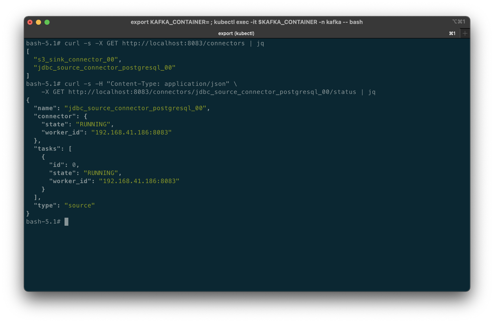
Errors preventing the connector from starting correctly will be displayed using the /status endpoint, as shown in the example below. In this case, the Kubernetes Service Account associated with the pod lacked the proper IAM permissions to the Amazon S3 target bucket.

Confirming Success of Connectors #1
The entire contents of the three tables will be exported from RDS to Kafka by the source connector, then exported from Kafka to S3 by the sink connector. To confirm the source connector worked, verify the existence of three new Kafka topics that should have been created: pagila.public.address, pagila.public.city, and pagila.public.country.
bin/kafka-topics.sh --list \
  --bootstrap-server $BBROKERS \
  --command-config config/client-iam.properties \
  | grep pagila.public.
To confirm the sink connector worked, verify the new S3 objects have been created in the data lake’s S3 bucket. If you use the AWS CLI v2’s s3 API, we can view the contents of our target S3 bucket:
aws s3api list-objects \
  --bucket your-s3-bucket \
  --query 'Contents[].{Key: Key}' \
  --output text
You should see approximately 15 new S3 objects (JSON files) in the S3 bucket, whose keys are organized by their topic names. The sink connector flushes new data to S3 every 100 records, or 60 seconds.
You could also use the AWS Management Console to view the S3 bucket’s contents.

Use the Amazon S3 console’s ‘Query with S3 Select’ to view the data contained in the JSON-format files. Alternately, you can use the s3 API:
export SINK_BUCKET="your-s3-bucket"
export KEY="topics/pagila.public.address/partition=0/pagila.public.address+0+0000000100.json"
aws s3api select-object-content \
    --bucket $SINK_BUCKET \
    --key $KEY \
    --expression "select * from s3object limit 5" \
    --expression-type "SQL" \
    --input-serialization '{"JSON": {"Type": "DOCUMENT"}, "CompressionType": "NONE"}' \
    --output-serialization '{"JSON": {}}' "output.json" \
  && cat output.json | jq \
  && rm output.json
For example, the address table’s data will look similar to the following using the ‘Query with S3 Select’ feature via the console or API:
{
  "address_id": 100,
  "address": "1308 Arecibo Way",
  "address2": "",
  "district": "Georgia",
  "city_id": 41,
  "postal_code": "30695",
  "phone": "6171054059",
  "last_update": 1487151930000
}
{
  "address_id": 101,
  "address": "1599 Plock Drive",
  "address2": "",
  "district": "Tete",
  "city_id": 534,
  "postal_code": "71986",
  "phone": "817248913162",
  "last_update": 1487151930000
}
{
  "address_id": 102,
  "address": "669 Firozabad Loop",
  "address2": "",
  "district": "Abu Dhabi",
  "city_id": 12,
  "postal_code": "92265",
  "phone": "412903167998",
  "last_update": 1487151930000
}
Congratulations, you have successfully imported data from a relational database into your data lake using Kafka Connect!
Connector Source #2
Create a new file or modify config/jdbc_source_connector_postgresql_01.json. Modify lines 3–5, as shown below, to reflect your RDS instance connection details.
This second Kafka Connect source connector also uses Confluent’s Kafka Connect JDBC Source connector to export data from the just address table with a JDBC driver and import that data into a new Kafka topic, pagila.public.alt.address. The difference with this source connector is transforms, known as Single Message Transformations (SMTs). SMTs are applied to messages as they flow through Connect from RDS to Kafka.
In this connector, there are four transforms, which perform the following common functions:
- Extract
address_idinteger field as the Kafka message key, as detailed in this blog post by Confluence (see ‘Setting the Kafka message key’). - Append Kafka topic name into message as a new static field;
- Append database name into message as a new static field;
Connector Sink #2
Create a new file or modify config/s3_sink_connector_01.json. Modify line 6, as shown below, to reflect your Amazon S3 bucket name.
This second sink connector is nearly identical to the first sink connector, except it only exports data from a single Kafka topic, pagila.public.alt.address, into S3.
Deploy Connectors #2
Deploy the second set of source and sink connectors using the Kafka Connect REST Interface, exactly like the first pair.
curl -s -d @"config/jdbc_source_connector_postgresql_01.json" \
    -H "Content-Type: application/json" \
    -X PUT http://localhost:8083/connectors/jdbc_source_connector_postgresql_01/config | jq
curl -s -d @"config/s3_sink_connector_01.json" \
    -H "Content-Type: application/json" \
    -X PUT http://localhost:8083/connectors/s3_sink_connector_01/config | jq
Confirming Success of Connectors #2
Use the same commands as before to confirm the new set of connectors are deployed and running, alongside the first set, for a total of four connectors.
curl -s -X GET http://localhost:8083/connectors | \
  jq '. | sort_by(.)'
curl -s -H "Content-Type: application/json" \
    -X GET http://localhost:8083/connectors/jdbc_source_connector_postgresql_01/status | jq
curl -s -H "Content-Type: application/json" \
    -X GET http://localhost:8083/connectors/s3_sink_connector_01/status | jq

To view the results of the first transform, extracting the address_id integer field as the Kafka message key, we can use a Kafka command-line consumer:
bin/kafka-console-consumer.sh \
  --topic pagila.public.alt.address \
  --offset 102 --partition 0 --max-messages 5 \
  --property print.key=true --property print.value=true \
  --property print.offset=true --property print.partition=true \
  --property print.headers=false --property print.timestamp=false \
  --bootstrap-server $BBROKERS \
  --consumer.config config/client-iam.properties
In the output below, note the beginning of each message, which displays the Kafka message key, identical to the address_id. For example, {"type":"int32","optional":false},"payload":100}.

topicExaming the Amazon S3 bucket using the AWS Management Console or the CLI, you should note the fourth set of S3 objects within the /topics/pagila.public.alt.address/ object key prefix.

Use the Amazon S3 console’s ‘Query with S3 Select’ to view the data contained in the JSON-format files. Alternately, you can use the s3 API:
export SINK_BUCKET="your-s3-bucket"
export KEY="topics/pagila.public.alt.address/partition=0/pagila.public.address+0+0000000100.json"
aws s3api select-object-content \
    --bucket $SINK_BUCKET \
    --key $KEY \
    --expression "select * from s3object limit 5" \
    --expression-type "SQL" \
    --input-serialization '{"JSON": {"Type": "DOCUMENT"}, "CompressionType": "NONE"}' \
    --output-serialization '{"JSON": {}}' "output.json" \
  && cat output.json | jq \
  && rm output.json
In the sample data below, note the two new fields that have been appended into each record, a result of the Kafka Connector transforms:
{
  "address_id": 100,
  "address": "1308 Arecibo Way",
  "address2": "",
  "district": "Georgia",
  "city_id": 41,
  "postal_code": "30695",
  "phone": "6171054059",
  "last_update": 1487151930000,
  "message_topic": "pagila.public.alt.address",
  "message_source": "pagila"
}
{
  "address_id": 101,
  "address": "1599 Plock Drive",
  "address2": "",
  "district": "Tete",
  "city_id": 534,
  "postal_code": "71986",
  "phone": "817248913162",
  "last_update": 1487151930000,
  "message_topic": "pagila.public.alt.address",
  "message_source": "pagila"
}
{
  "address_id": 102,
  "address": "669 Firozabad Loop",
  "address2": "",
  "district": "Abu Dhabi",
  "city_id": 12,
  "postal_code": "92265",
  "phone": "412903167998",
  "last_update": 1487151930000,
  "message_topic": "pagila.public.alt.address",
  "message_source": "pagila"
}
Congratulations, you have successfully imported more data from a relational database into your data lake, including performing a simple series of transforms using Kafka Connect!
Connector Source #3
Create or modify config/jdbc_source_connector_postgresql_02.json. Modify lines 3–5, as shown below, to reflect your RDS instance connection details.
Unlike the first two source connectors that export data from tables, this connector uses a SELECT query to export data from the Pagila database’s address , city, and country tables and import the results of that SQL query data into a new Kafka topic, pagila.public.alt.address. The SQL query in the source connector’s configuration is as follows:
SELECT a.address_id,
             a.address,
             a.address2,
             city.city,
             a.district,
             a.postal_code,
             country.country,
             a.phone,
             a.last_update
      FROM address AS a
               INNER JOIN city ON a.city_id = city.city_id
               INNER JOIN country ON country.country_id = city.country_id
      ORDER BY address_id) AS addresses
The final parameterized query, executed by the source connector, which allows it to detect changes based on the last_update field is as follows:
SELECT *
FROM (SELECT a.address_id,
             a.address,
             a.address2,
             city.city,
             a.district,
             a.postal_code,
             country.country,
             a.phone,
             a.last_update
      FROM address AS a
               INNER JOIN city ON a.city_id = city.city_id
               INNER JOIN country ON country.country_id = city.country_id
      ORDER BY address_id) AS addresses
WHERE "last_update" > ?
  AND "last_update" < ?
ORDER BY "last_update" ASC
Connector Sink #3
Create or modify config/s3_sink_connector_02.json. Modify line 6, as shown below, to reflect your Amazon S3 bucket name.
This sink connector is significantly different than the previous two sink connectors. In addition to leveraging SMTs in the corresponding source connector, we are also using them in this sink connector. The sink connect appends three arbitrary static fields to each record as it is written to Amazon S3 — message_source, message_source_engine, and environment using the InsertField transform. The sink connector also renames the district field to state_province using the ReplaceField transform.
The first two sink connectors wrote uncompressed JSON-format files to Amazon S3. This third sink connector optimizes the data imported into S3 for downstream data analytics. The sink connector writes GZIP-compressed Apache Parquet files to Amazon S3. In addition, the compressed Parquet files are partitioned by the country field. Using a columnar file format, compression, and partitioning, queries against the data should be faster and more efficient.
Deploy Connectors #3
Deploy the final source and sink connectors using the Kafka Connect REST Interface, exactly like the first two pairs.
curl -s -d @"config/jdbc_source_connector_postgresql_02.json" \
    -H "Content-Type: application/json" \
    -X PUT http://localhost:8083/connectors/jdbc_source_connector_postgresql_02/config | jq
curl -s -d @"config/s3_sink_connector_02.json" \
    -H "Content-Type: application/json" \
    -X PUT http://localhost:8083/connectors/s3_sink_connector_02/config | jq
Confirming Success of Connectors #3
Use the same commands as before to confirm the new set of connectors are deployed and running, alongside the first two sets, for a total of six connectors.
curl -s -X GET http://localhost:8083/connectors | \
  jq '. | sort_by(.)'
curl -s -H "Content-Type: application/json" \
    -X GET http://localhost:8083/connectors/jdbc_source_connector_postgresql_02/status | jq
curl -s -H "Content-Type: application/json" \
    -X GET http://localhost:8083/connectors/s3_sink_connector_02/status | jq

Reviewing the messages within the newpagila.query topic, note the message_topic field has been appended to the message by the source connector but not message_source, message_source_engine, and environment fields. The sink connector appends these fields as it writes the messages to S3. Also, note the district field has yet to be renamed by the sink connector to state_province.

pagila.query topicExaming the Amazon S3 bucket, again, you should note the fifth set of S3 objects within the /topics/pagila.query/ object key prefix. The Parquet-format files within are partitioned by country.

Within each country partition, there are Parquet files whose records contain addresses within those countries.

Use the Amazon S3 console’s ‘Query with S3 Select’ again to view the data contained in the Parquet-format files. Alternately, you can use the s3 API:
export SINK_BUCKET="your-s3-bucket"
export KEY="topics/pagila.query/country=United States/pagila.query+0+0000000003.gz.parquet"
aws s3api select-object-content \
    --bucket $SINK_BUCKET \
    --key $KEY \
    --expression "select * from s3object limit 5" \
    --expression-type "SQL" \
    --input-serialization '{"Parquet": {}}' \
    --output-serialization '{"JSON": {}}' "output.json" \
  && cat output.json | jq \
  && rm output.json
In the sample data below, note the four new fields that have been appended into each record, a result of the source and sink connector SMTs. Also, note the renamed district field:
{
  "address_id": 599,
  "address": "1895 Zhezqazghan Drive",
  "address2": "",
  "city": "Garden Grove",
  "state_province": "California",
  "postal_code": "36693",
  "country": "United States",
  "phone": "137809746111",
  "last_update": "2017-02-15T09:45:30.000Z",
  "message_topic": "pagila.query",
  "message_source": "pagila",
  "message_source_engine": "postgresql",
  "environment": "development"
}
{
  "address_id": 6,
  "address": "1121 Loja Avenue",
  "address2": "",
  "city": "San Bernardino",
  "state_province": "California",
  "postal_code": "17886",
  "country": "United States",
  "phone": "838635286649",
  "last_update": "2017-02-15T09:45:30.000Z",
  "message_topic": "pagila.query",
  "message_source": "pagila",
  "message_source_engine": "postgresql",
  "environment": "development"
}
{
  "address_id": 18,
  "address": "770 Bydgoszcz Avenue",
  "address2": "",
  "city": "Citrus Heights",
  "state_province": "California",
  "postal_code": "16266",
  "country": "United States",
  "phone": "517338314235",
  "last_update": "2017-02-15T09:45:30.000Z",
  "message_topic": "pagila.query",
  "message_source": "pagila",
  "message_source_engine": "postgresql",
  "environment": "development"
}
Record Updates and Query-based CDC
What happens when we change data within the tables that Kafka Connect is polling every 5 seconds? To answer this question, let’s make a few DML changes:
-- update address field
UPDATE public.address
SET address = '123 CDC Test Lane'
WHERE address_id = 100;
-- update address2 field
UPDATE public.address
SET address2 = 'Apartment #2201'
WHERE address_id = 101;
-- second update to same record
UPDATE public.address
SET address2 = 'Apartment #2202'
WHERE address_id = 101;
-- insert new country
INSERT INTO public.country (country)
values ('Wakanda');
-- should be 110
SELECT country_id FROM country WHERE country='Wakanda';
-- insert new city
INSERT INTO public.city (city, country_id)
VALUES ('Birnin Zana', 110);
-- should be 601
SELECT city_id FROM public.city WHERE country_id=110;
-- update city_id to new city_id
UPDATE public.address
SET phone = city_id = 601
WHERE address_id = 102;
-- second update to same record
UPDATE public.address
SET district = 'Lake Turkana'
WHERE address_id = 102;
-- delete an address record
UPDATE public.customer
SET address_id = 200
WHERE customer_id IN (
    SELECT customer_id FROM customer WHERE address_id = 104);
DELETE
FROM public.address
WHERE address_id = 104;
To see how these changes propagate, first, examine the Kafka Connect logs. Below, we see example log events corresponding to some of the database changes shown above. The three Kafka Connect source connectors detect changes, which are exported from PostgreSQL to Kafka. The three sink connectors then write these changes to new JSON and Parquet files to the target S3 bucket.

Viewing Data in the Data Lake
A convenient way to examine both the existing data and ongoing data changes in our data lake is to crawl and catalog the S3 bucket’s contents with AWS Glue, then query the results with Amazon Athena. AWS Glue’s Data Catalog is an Apache Hive-compatible, fully-managed, persistent metadata store. AWS Glue can store the schema, metadata, and location of our data in S3. Amazon Athena is a serverless Presto-based (PrestoDB) ad-hoc analytics engine, which can query AWS Glue Data Catalog tables and the underlying S3-based data.

When writing Parquet into partitions, one shortcoming of the Kafka Connect S3 sink connector is duplicate column names in AWS Glue. As a result, any columns used as partitions are duplicated in the Glue Data Catalog’s database table schema. The issue will result in an error similar to HIVE_INVALID_METADATA: Hive metadata for table pagila_query is invalid: Table descriptor contains duplicate columns when performing queries. To remedy this, predefine the table and the table’s schema. Alternately, edit the Glue Data Catalog table’s schema after crawling and remove the duplicate, non-partition column(s). Below, that would mean removing duplicate country column 7.

Performing a typical SQL SELECT query in Athena will return all of the original records as well as the changes we made earlier as duplicate records (same address_id primary key).

SELECT address_id, address, address2, city, state_province,
         postal_code, country, last_update
FROM "pagila_kafka_connect"."pagila_query"
WHERE address_id BETWEEN 100 AND 105
ORDER BY address_id;
Note the original records for address_id 100–103 as well as each change we made earlier. The last_update field reflects the date and time the record was created or updated. Also, note the record with address_id 104 in the query results. This is the record we deleted from the Pagila database.
To view only the most current data, we can use Athena’s ROW_NUMBER() function:
SELECT address_id, address, address2, city, state_province,
         postal_code, country, last_update
FROM (SELECT *, ROW_NUMBER() OVER (
                  PARTITION BY address_id
                  ORDER BY last_UPDATE DESC) AS row_num
      FROM "pagila_kafka_connect"."pagila_query") AS x
WHERE x.row_num = 1
  AND address_id BETWEEN 100 AND 105
ORDER BY address_id;
Now, we only see the latest records. Unfortunately, the record we deleted with address_id 104 is still present in the query results.
Using log-based CDC with Debezium, as opposed to query-based CDC, we would have received a record in S3 that indicated the delete. The null value message, shown below, is referred to as a tombstone message in Kafka. Note the ‘before’ syntax with the delete record as opposed to the ‘after’ syntax we observed earlier with the update record.
{
  "before": {
    "address": "",
    "address2": null,
    "phone": "",
    "district": "",
    "last_update": "1970-01-01T00:00:00Z",
    "address_id": 104,
    "postal_code": null,
    "city_id": 0
  },
  "source": {
    "schema": "public",
    "sequence": "[\"1101256482032\",\"1101256482032\"]",
    "xmin": null,
    "connector": "postgresql",
    "lsn": 1101256483936,
    "name": "pagila",
    "txId": 17137,
    "version": "1.6.1.Final",
    "ts_ms": 1628864251512,
    "snapshot": "false",
    "db": "pagila",
    "table": "address"
  },
  "op": "d",
  "ts_ms": 1628864251671
}
An inefficient solution to duplicates and deletes with query-based CDC would be to bulk ingest the entire query result set from the Pagila database each time instead of only the changes based on the last_update field. Performing an unbounded query repeatedly on a huge dataset would negatively impact database performance. Notwithstanding, you would still end up with duplicates in the data lake unless you first purged the data in S3 before re-importing the new query results.
Data Movement
Using Amazon Athena, we can easily write the results of our ROW_NUMBER() query back to the data lake for further enrichment or analysis. Athena’s CREATE TABLE AS SELECT (CTAS) SQL statement creates a new table in Athena (an external table in AWS Glue Data Catalog) from the results of a SELECT statement in the subquery. Athena stores data files created by the CTAS statement in a specified location in Amazon S3 and created a new AWS Glue Data Catalog table to store the result set’s schema and metadata information. CTAS supports several file formats and storage options.
Wrapping the last query in Athena’s CTAS statement, as shown below, we can write the query results as SNAPPY-compressed Parquet-format files, partitioned by country, to a new location in the Amazon S3 bucket. Using common data lake terminology, I will refer to the resulting filtered and cleaned dataset as refined or silver instead of the raw ingestion or bronze data originating from our data source, PostgreSQL, via Kafka.
CREATE TABLE pagila_kafka_connect.pagila_query_processed
WITH (
  format='PARQUET',
  parquet_compression='SNAPPY',
  partitioned_by=ARRAY['country'],
  external_location='s3://your-s3-bucket/processed/pagila_query'
) AS
SELECT address_id, last_update, address, address2, city,
         state_province, postal_code, country
FROM (SELECT *, ROW_NUMBER() OVER (
                  PARTITION BY address_id
                  ORDER BY last_update DESC) AS row_num
      FROM "pagila_kafka_connect"."pagila_query") AS x
WHERE x.row_num = 1 AND address_id BETWEEN 0 and 100
ORDER BY address_id;
Examing the Amazon S3 bucket, on last time, you should new set of S3 objects within the /processed/pagila_query/ key path. The Parquet-format files, partitioned by country, are the result of the CTAS query.

We should now see a new table in the same AWS Glue Data Catalog containing metadata, location, and schema information about the data we wrote to S3 using the CTAS query. We can perform additional queries on the processed data.

ACID Transactions with a Data Lake
To fully take advantage of CDC and maximize the freshness of data in the data lake, we would also need to adopt modern data lake file formats like Apache Hudi, Apache Iceberg, or Delta Lake, along with analytics engines such as Apache Spark with Spark Structured Streaming to process the data changes. Using these technologies, it is possible to perform record-level updates and deletes of data in an object store like Amazon S3. Hudi, Iceberg, and Delta Lake offer features including ACID transactions, schema evolution, upserts, deletes, time travel, and incremental data consumption in a data lake. ELT engines like Spark can read streaming Debezium-generated CDC messages from Kafka and process those changes using Hudi, Iceberg, or Delta Lake.
Conclusion
This post explored how CDC could help us hydrate data from an Amazon RDS database into an Amazon S3-based data lake. We leveraged the capabilities of Amazon EKS, Amazon MSK, and Apache Kafka Connect. We learned about query-based CDC for capturing ongoing changes to the source data. In a subsequent post, we will explore log-based CDC using Debezium and see how data lake file formats like Apache Avro, Apache Hudi, Apache Iceberg, and Delta Lake can help us manage the data in our data lake.
This blog represents my own viewpoints and not of my employer, Amazon Web Services (AWS). All product names, logos, and brands are the property of their respective owners.
Gary Stafford
AWS Area Principal Solutions Architect | 10x AWS Certified Pro | DevOps | Data/ML | Serverless | Polyglot Developer | Former ThoughtWorks and Accenture
