Posts Tagged ARM
GTM Stack: Exploring IoT Data Analytics at the Edge with Grafana, Mosquitto, and TimescaleDB on ARM-based Architectures
Posted by Gary A. Stafford in Big Data, IoT, Python, Raspberry Pi, Software Development on October 12, 2020
In the following post, we will explore the integration of several open-source software applications to build an IoT edge analytics stack, designed to operate on ARM-based edge nodes. We will use the stack to collect, analyze, and visualize IoT data without first shipping the data to the Cloud or other external systems.

The Edge
Edge computing is a fast-growing technology trend, which involves pushing compute capabilities to the edge. Wikipedia describes edge computing as a distributed computing paradigm that brings computation and data storage closer to the location needed to improve response times and save bandwidth. The term edge commonly refers to a compute node at the edge of a network (edge device), sitting in close proximity to the source a data and between that data source and external system such as the Cloud.
In his recent post, 3 Advantages (And 1 Disadvantage) Of Edge Computing, well-known futurist Bernard Marr argues reduced bandwidth requirements, reduced latency, and enhanced security and privacy as three primary advantages of edge computing. Due to techniques like data downsampling, Marr advises one potential disadvantage of edge computing is that important data could end up being overlooked and discarded in the quest to save bandwidth and reduce latency.
David Ricketts, Head of Marketing at Quiss Technology PLC, estimates in his post, Cloud and Edge Computing — The Stats You Need to Know for 2018, the global edge computing market is expected to reach USD 6.72 billion by 2022 at a compound annual growth rate of a whopping 35.4 percent. Realizing the market potential, many major Cloud providers, edge device manufacturers, and integrators are rapidly expanding their edge compute capabilities. AWS, for example, currently offers more than a dozen services in the edge computing category.
Internet of Things
Edge computing is frequently associated with the Internet of Things (IoT). IoT devices, industrial equipment, and sensors generate data, which is transmitted to other internal and external systems, often by way of edge nodes, such as an IoT Gateway. IoT devices typically generate time-series data. According to Wikipedia, a time series is a set of data points indexed in time order — a sequence taken at successive equally spaced points in time. IoT devices typically generate continuous high-volume streams of time-series data, often on the scale of millions of data points per second. IoT data characteristics require IoT platforms to minimally support temporal accuracy, high-volume ingestion and processing, efficient data compression and downsampling, and real-time querying capabilities.
The IoT devices and the edge devices, such as IoT Gateways, which aggregate and transmit IoT data from these devices to external systems, are generally lower-powered, with limited processor, memory, and storage capabilities. Accordingly, IoT platforms must satisfy all the requirements of IoT data while simultaneously supporting resource-constrained environments.
IoT Analytics at the Edge
Leading Cloud providers AWS, Azure, Google Cloud, IBM Cloud, Oracle Cloud, and Alibaba Cloud all offer IoT services. Many offer IoT services with edge computing capabilities. AWS offers AWS IoT Greengrass. Greengrass provides local compute, messaging, data management, sync, and ML inference capabilities to edge devices. Azure offers Azure IoT Edge. Azure IoT Edge provides the ability to run AI, Azure and third-party services, and custom business logic on edge devices using standard containers. Google Cloud offers Edge TPU. Edge TPU (Tensor Processing Unit) is Google’s purpose-built application-specific integrated circuit (ASIC), designed to run AI at the edge.
IoT Analytics
Many Cloud providers also offer IoT analytics as part of their suite of IoT services, although not at the edge. AWS offers AWS IoT Analytics, while Azure has Azure Time Series Insights. Google provides IoT analytics, indirectly, through downstream analytic systems and ad hoc analysis using Google BigQuery or advanced analytics and machine learning with Cloud Machine Learning Engine. These services generally all require data to be transmitted to the Cloud for analytics.

The ability to analyze IoT data at the edge, as data is streamed in real-time, is critical to a rapid feedback loop. IoT edge analytics can accelerate anomaly detection, improve predictive maintenance capabilities, and expedite proactive inventory replenishment.
The IoT Edge Analytics Stack
In my opinion, the ideal IoT edge analytics stack is comprised of lightweight, purpose-built, easily deployable and manageable, platform- and programming language-agnostic, open-source software components. The minimal IoT edge analytics stack should include a lightweight message broker, a time-series database, an ANSI-standard ad-hoc query engine, and a data visualization tool. Each component should be purpose-built for IoT.
Lightweight Message Broker
We will use Eclipse Mosquitto as our message broker. According to the project’s description, Mosquitto is an open-source message broker that implements the Message Queuing Telemetry Transport (MQTT) protocol versions 5.0, 3.1.1, and 3.1. Mosquitto is lightweight and suitable for use on all devices from low power single board computers (SBCs) to full servers.
MQTT Client Library
We will interact with Mosquitto using Eclipse Paho. According to the project, the Eclipse Paho project provides open-source, mainly client-side implementations of MQTT and MQTT-SN in a variety of programming languages. MQTT and MQTT for Sensor Networks (MQTT-SN) are lightweight publish/subscribe messaging transports for TCP/IP and connectionless protocols, such as UDP, respectively.
We will be using Paho’s Python Client. The Paho Python Client provides a client class with support for both MQTT v3.1 and v3.1.1 on Python 2.7 or 3.x. The client also provides helper functions to make publishing messages to an MQTT server straightforward.
Time-Series Database
Time-series databases are optimal for storing IoT data. According to InfluxData, makers of a leading time-series database, InfluxDB, a time-series database (TSDB), is a database optimized for time-stamped or time-series data. Time series data are simply measurements or events that are tracked, monitored, downsampled, and aggregated over time. Jiao Xian, of Alibaba Cloud, has authored an insightful post on the time-series database ecosystem, What Are Time Series Databases? A few leading Cloud providers offer purpose-built time-series databases, though they are not available at the edge. AWS offers Amazon Timestream and Alibaba Cloud offers Time Series Database.
InfluxDB is an excellent choice for a time-series database. It was my first choice, along with TimescaleDB, when developing this stack. However, InfluxDB Flux’s apparent incompatibilities with some ARM-based architectures ruled it out for inclusion in the stack for this particular post.
We will use TimescaleDB as our time-series database. TimescaleDB is the leading open-source relational database for time-series data. Described as ‘PostgreSQL for time-series,’ TimescaleDB is based on PostgreSQL, which provides full ANSI SQL, rock-solid reliability, and a massive ecosystem. TimescaleDB claims to achieve 10–100x faster queries than PostgreSQL, InfluxDB, and MongoDB, with native optimizations for time-series analytics.
TimescaleDB claims to achieve 10–100x faster queries than PostgreSQL, InfluxDB, and MongoDB, with native optimizations for time-series analytics.
TimescaleDB is designed for performing analytical queries, both through its native support for PostgreSQL’s full range of SQL functionality, as well as additional functions native to TimescaleDB. These time-series optimized functions include Median/Percentile, Cumulative Sum, Moving Average, Increase, Rate, Delta, Time Bucket, Histogram, and Gap Filling.
Ad-hoc Data Query Engine
We have the option of using psql, the terminal-based front-end to PostgreSQL, to execute ad-hoc queries against TimescaleDB. The psql front-end enables you to enter queries interactively, issue them to PostgreSQL, and see the query results.

We also have the option of using pgAdmin, specifically the biarms/pgadmin4 Docker version, to execute ad-hoc queries and perform most other database tasks. pgAdmin is the most popular open-source administration and development platform for PostgreSQL. While several popular Docker versions of pgAdmin only support Linux AMD64 architectures, the biarms/pgadmin4 Docker version supports ARM-based devices.


Data Visualization
For data visualization, we will use Grafana. Grafana allows you to query, visualize, alert on, and understand metrics no matter where they are stored. With Grafana, you can create, explore, and share dashboards, fostering a data-driven culture. Grafana allows you to define thresholds visually and get notified via Slack, PagerDuty, and more. Grafana supports dozens of data sources, including MySQL, PostgreSQL, Elasticsearch, InfluxDB, TimescaleDB, Graphite, Prometheus, Google BigQuery, GraphQL, and Oracle. Grafana is extensible through a large collection of plugins.
Edge Deployment and Management Platform
Docker introduced the current industry standard for containers in 2013. Docker containers are a standardized unit of software that allows developers to isolate apps from their environment. We will use Docker to deploy the IoT edge analytics stack, referred to herein as the GTM Stack, composed of containerized versions of Eclipse Mosquitto, TimescaleDB, and Grafana, and pgAdmin, to an ARM-based edge node. The acronym, GTM, comes from the three primary OSS projects composing the stack. The acronym also suggests Greenwich Mean Time, relating to the precise time-series nature of IoT data.
Running Docker Engine in swarm mode, we can use Docker to deploy the complete IoT edge analytics stack to the swarm, running on the edge node. The deploy command accepts a stack description in the form of a Docker Compose file, a YAML file used to configure the application’s services. With a single command, we can create and start all the services from the configuration file.
Source Code
All source code for this post is available on GitHub. Use the following command to git clone a local copy of the project.
IoT Devices
For this post, I have deployed three Linux ARM-based IoT devices, each connected to a sensor array. Each sensor array contains multiple analog and digital sensors. The sensors record temperature, humidity, air quality (liquefied petroleum gas (LPG), carbon monoxide (CO), and smoke), light, and motion. For more information on the IoT device and sensor hardware involved, please see my previous post: Getting Started with IoT Analytics on AWS.
Each ARM-based IoT device is running a small Python3-based script, sensor_data_to_mosquitto.py, shown below.
The IoT devices’ script implements the Eclipse Paho MQTT Python client library. An MQTT message containing simultaneous readings from each sensor is sent to a Mosquitto topic on the edge node, at a configurable frequency.
IoT Edge Node
For this post, I have deployed a single Linux ARM-based edge node. The three IoT devices, containing sensor arrays, communicate with the edge node over Wi-Fi. The IoT devices could easily use an alternative communication protocol, such as BLE, LoRaWAN, or Ethernet. For more information on BLE and LoRaWAN, please see some of my previous posts: LoRa and LoRaWAN for IoT: Getting Started with LoRa and LoRaWAN Protocols for Low Power, Wide Area Networking of IoT and BLE and GATT for IoT: Getting Started with Bluetooth Low Energy (BLE) and Generic Attribute Profile (GATT) Specification for IoT.
The edge node is also running a small Python3-based script, mosquitto_to_timescaledb.py, shown below.
Similar to the IoT devices, the edge node’s script implements the Eclipse Paho MQTT Python client library. The script pulls MQTT messages off a Mosquitto topic(s), serializes the message payload to JSON, and writes the payload’s data to the TimescaleDB database. The edge node’s script accepts several arguments, which allow you to configure necessary Mosquitto and TimescaleDB variables.
Why not use Telegraf?
Telegraf is a plugin-driven agent that collects, processes, aggregates, and writes metrics. There is a Telegraf output plugin, the PostgreSQL and TimescaleDB Output Plugin for Telegraf, produced by TimescaleDB. The plugin could replace the need to manage and maintain the above script. However, I chose not to use it because it is not yet an official Telegraf plugin. If the plugin was included in a Telegraf release, I would certainly encourage its use.
Script Management
Both the Linux-based IoT devices and the edge node run systemd system and service manager. To ensure the Python scripts keep running in the case of a system restart, we define a systemd unit. Units are the objects that systemd knows how to manage. These are basically a standardized representation of system resources that can be managed by the suite of daemons and manipulated by the provided utilities. Each script has a systemd unit files. Below, we see the gtm_stack_mosquitto unit file, gtm_stack_mosquitto.service.
The gtm_stack_mosq_to_tmscl unit file, gtm_stack_mosq_to_tmscl.service, is nearly identical.
To install the gtm_stack_mosquitto.service systemd unit file on each IoT device, use the following commands.
Installing the gtm_stack_mosq_to_tmscl.service unit file on the edge node is nearly identical.
Docker Stack
The edge node runs the GTM Docker stack, stack.yml, in a swarm. As discussed earlier, the stack contains four containers: Eclipse Mosquitto, TimescaleDB, and Grafana, along with pgAdmin. The Mosquitto, TimescaleDB, and Grafana containers have paths within the containers, bind-mounted to directories on the edge device. With bind-mounting, the container’s data will persist if the containers are removed and re-created. The containers are running on their own isolated overlay network.
The GTM Docker stack is installed using the following commands on the edge node. We will assume Docker and git are pre-installed on the edge node for this post.
First, we create the proper local directories on the edge device, which will be used to bind-mount to the container’s directories. Below, we see the bind-mounted local directories with the eventual container’s contents stored within them.

Next, we copy the custom Mosquitto configuration file, mosquitto.conf, included in the project, to the correct location on the edge device. Lastly, we initialize the Docker swarm and deploy the stack.

docker container ls command, showing the running GTM Stack containers
docker stats command, showing the resource consumption of GTM Stack containersTimescaleDB Setup
With the GTM stack running, we need to create a single Timescale hypertable, sensor_data, in the TimescaleDB demo_iot database, to hold the incoming IoT sensor data. Hypertables, according to TimescaleDB, are designed to be easy to manage and to behave like standard PostgreSQL tables. Hypertables are comprised of many interlinked “chunk” tables. Commands made to the hypertable automatically propagate changes down to all of the chunks belonging to that hypertable.
I suggest using psql to execute the required DDL statements, which will create the hypertable, as well as the proceeding views and database user permissions. All SQL statements are included in the project’s statements.sql file. One way to use psql is to install it on your local workstation, then use psql to connect to the remote edge node. I prefer to instantiate a local PostgreSQL Docker container instance running psql. I then use the local container’s psql client to connect to the edge node’s TimescaleDB database. For example, from my local machine, I run the following docker run command to connect to the edge node’s TimescaleDB database, on the edge node, located locally at 192.168.1.12.
Although not always practical, could also access psql from within the TimescaleDB Docker container, running on the actual edge node, using the following docker exec command.
TimescaleDB Continuous Aggregates
For this post’s demonstration, we need to create four TimescaleDB database views, which will be queried from an eventual Grafana Dashboard. The views are TimescaleDB Continuous Aggregates. According to Timescale, aggregate queries that touch large swathes of time-series data can take a long time to compute because the system needs to scan large amounts of data on every query execution. TimescaleDB continuous aggregates automatically calculate the results of a query in the background and materialize the results.
For example, in this post, we generate sensor data every five seconds from the three IoT devices. When visualizing a 24-hour period in Grafana, using continuous aggregates with an interval of one minute, we would reduce the total volume of data queried from ~51,840 rows to ~4,320 rows, a reduction of over 91%. The larger the time period or the number of IoT devices being analyzed, the more significant these savings will positively impact query performance.
A time_bucket on the time partitioning column of the hypertable is required in all continuous aggregate views. The time_bucket function, in this case, has a bucket width (interval) of 1 minute. The interval is configurable.
Limiting Grafana’s Access to IoT Data
Following the Grafana recommendation for database user permissions, we create a grafanareader PostgresSQL user, and limit the user’s access to the sensor_data table and the four views we created. Grafana will use this user’s credentials to perform SELECT queries of the TimescaleDB demo_iot database.
Grafana Dashboards
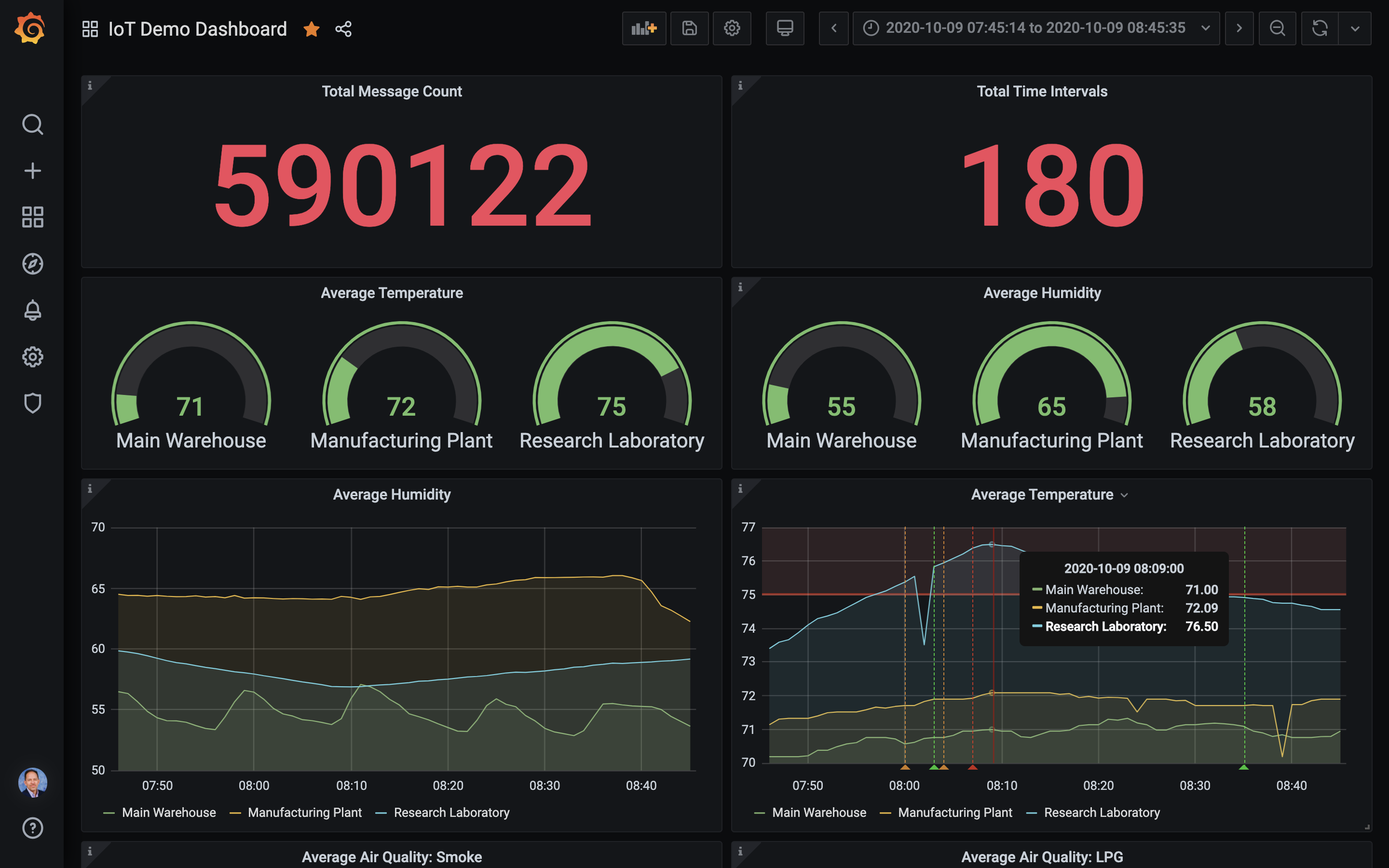
Using the TimescaleDB continuous aggregates we have created, we can quickly build a richly-featured dashboard in Grafana. Below we see a typical IoT Dashboard you might build to monitor the post’s IoT sensor data in near real-time. An exported version, dashboard_external_export.json, is included in the GitHub project.

Grafana’s documentation includes a comprehensive set of instructions for Using PostgreSQL in Grafana. To connect to the TimescaleDB database from Grafana, we use a PostgreSQL data source.

The data displayed in each Panel in the Grafana Dashboard is based on a SQL query. For example, the Average Temperature Panel might use a query similar to the example below. This particular query also converts Celcius to Fahrenheit. Note the use of Grafana Macros (e.g., $__time(), $__timeFilter()). Macros can be used within a query to simplify syntax and allow for dynamic parts.
SELECT
  $__time(bucket),
  device_id AS metric,
  ((avg_temp * 1.9) + 32) AS avg_temp
FROM temperature_humidity_summary_minute
WHERE
  $__timeFilter(bucket)
ORDER BY 1,2
Below, we see another example from the Average Humidity Panel. In this particular query, we might choose to validate the humidity data is within an acceptable range of 0%–100%.
SELECT
  $__time(bucket),
  device_id AS metric,
  avg_humidity
FROM temperature_humidity_summary_minute
WHERE
  $__timeFilter(bucket)
  AND avg_humidity >= 0.0
  AND avg_humidity <= 100.0
ORDER BY 1,2
Mobile Friendly
Grafana dashboards are mobile-friendly. Below we see two views of the dashboard, using the Chrome mobile browser on an Apple iPhone.

Grafana Alerts
Grafana allows Alerts to be created based on Rules you define in each Panel. If data values match the Rule’s conditions, which you pre-define, such as a temperature reading above a certain threshold for a set amount of time, an alert is sent to your choice of destinations. According to the Rule shown below, If the average temperature exceeds 75°F for a period of 5 minutes, an alert is sent.
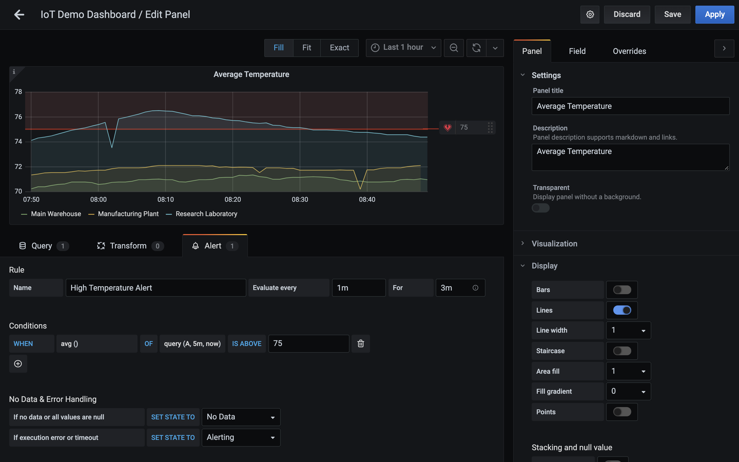
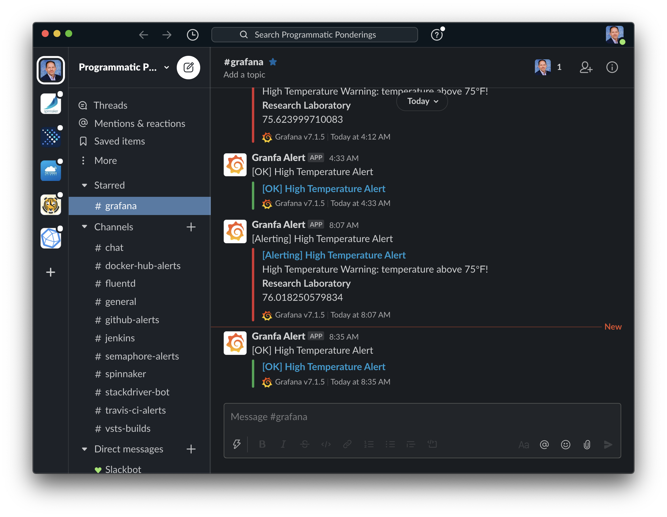
As demonstrated below, when the temperature in the laboratory began to exceed 75°F, the alert entered a ‘Pending’ state. If the temperature exceeded 75°F for the pre-determined period of 5 minutes, the alert status changed to ‘Alerting’, and an alert was sent. When the temperature dropped back below 75°F for the pre-determined period of 5 minutes, the alert status changed from ‘Alerting’ to ‘OK’, and a subsequent notification was sent.

There are currently 18 destinations available out-of-the-box with Grafana, including Slack, email, PagerDuty, webhooks, HipChat, and Microsoft Teams. We can use Grafana Alerts to notify the proper resources, in near real-time, if an issue is detected, based on the data. Below, we see an actual series of high-temperature alerts sent by Grafana to a Slack channel, followed by subsequent notifications as the temperature returned to normal.
Ad-hoc Queries
The ability to perform ad-hoc queries on the time-series IoT data is an essential feature of the IoT edge analytics stack. We can use psql or pgAdmin to perform ad-hoc queries against the TimescaleDB database. Below are examples of typical ad-hoc queries we might perform on the IoT sensor data. These example queries demonstrate TimescaleDB’s advanced analytical capabilities for working with time-series data, including Moving Average, Delta, Time Bucket, and Histogram.
Conclusion
In this post, we have explored the development of an IoT edge analytics stack, comprised of lightweight, purpose-built, easily deployable and manageable, platform- and programming language-agnostic, open-source software components. These components included Docker containerized versions of Eclipse Mosquitto, TimescaleDB, Grafana, and pgAdmin, referred to as the GTM Stack. Using the GTM stack, we collected, analyzed, and visualized IoT data, without first shipping the data to Cloud or other external systems.
This blog represents my own viewpoints and not of my employer, Amazon Web Services. All product names, logos, and brands are the property of their respective owners.
Object Tracking on the Raspberry Pi with C++, OpenCV, and cvBlob
Posted by Gary A. Stafford in Bash Scripting, C++ Development, Raspberry Pi on February 9, 2013
Use C++ with OpenCV and cvBlob to perform image processing and object tracking on the Raspberry Pi, using a webcam.
Source code and compiled samples are now available on GitHub. The below post describes the original code on the ‘Master’ branch. As of May 2014, there is a revised and improved version of the project on the ‘rev05_2014’ branch, on GitHub. The README.md details the changes and also describes how to install OpenCV, cvBlob, and all dependencies!
Introduction
As part of a project with a local FIRST Robotics Competition (FRC) Team, I’ve been involved in developing a Computer Vision application for use on the Raspberry Pi. Our FRC team’s goal is to develop an object tracking and target acquisition application that could be run on the Raspberry Pi, as opposed to the robot’s primary embedded processor, a National Instrument’s NI cRIO-FRC II. We chose to work in C++ for its speed, We also decided to test two popular open-source Computer Vision (CV) libraries, OpenCV and cvBlob.
Due to its single ARM1176JZF-S 700 MHz ARM processor, a significant limitation of the Raspberry Pi is the ability to perform complex operations in real-time, such as image processing. In an earlier post, I discussed Motion to detect motion with a webcam on the Raspberry Pi. Although the Raspberry Pi was capable of running Motion, it required a greatly reduced capture size and frame-rate. And even then, the Raspberry Pi’s ability to process the webcam’s feed was very slow. I had doubts it would be able to meet the processor-intense requirements of this project.
Development for the Raspberry Pi
Using C++ in NetBeans 7.2.1 on Ubuntu 12.04.1 LTS and 12.10, I wrote several small pieces of code to demonstrate the Raspberry Pi’s ability to perform basic image processing and object tracking. Parts of the follow code are based on several OpenCV and cvBlob code examples, found in my research. Many of those examples are linked on the end of this article. Examples of cvBlob are especially hard to find.
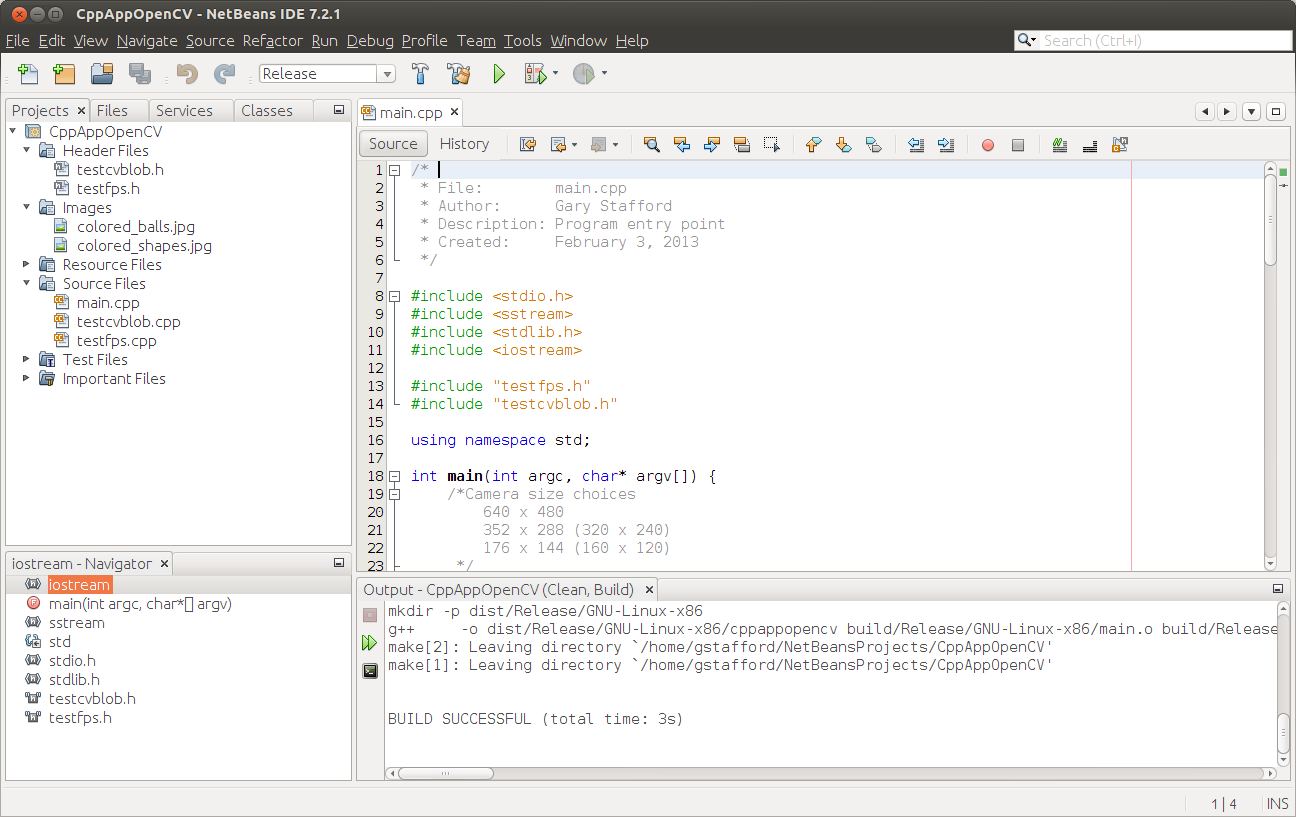
Project in NetBeans
The Code
There are five files: ‘main.cpp’, ‘testfps.cpp (testfps.h)’, and ‘testcvblob.cpp (testcvblob.h)’. The main.cpp file’s main method calls the test methods in the other two files. The cvBlob library only works with the pre-OpenCV 2.0. Therefore, I wrote all the code using the older objects and methods. The code is not written using the latest OpenCV 2.0 conventions. For example, cvBlob uses 1.0’s ‘IplImage’ image type instead 2.0’s newer ‘CvMat’ image type. My next projects is to re-write the cvBlob code to use OpenCV 2.0 conventions and/or find a newer library. The cvBlob library offered so many advantages, I felt not using the newer OpenCV 2.0 features was still worthwhile.
Main Program Method (main.cpp)
| /* | |
| * File: main.cpp | |
| * Author: Gary Stafford | |
| * Description: Program entry point | |
| * Created: February 3, 2013 | |
| */ | |
| #include <stdio.h> | |
| #include <sstream> | |
| #include <stdlib.h> | |
| #include <iostream> | |
| #include "testfps.hpp" | |
| #include "testcvblob.hpp" | |
| using namespace std; | |
| int main(int argc, char* argv[]) { | |
| int captureMethod = 0; | |
| int captureWidth = 0; | |
| int captureHeight = 0; | |
| if (argc == 4) { // user input parameters with call | |
| captureMethod = strtol(argv[1], NULL, 0); | |
| captureWidth = strtol(argv[2], NULL, 0); | |
| captureHeight = strtol(argv[3], NULL, 0); | |
| } else { // user did not input parameters with call | |
| cout << endl << "Demonstrations/Tests: " << endl; | |
| cout << endl << "(1) Test OpenCV - Show Webcam" << endl; | |
| cout << endl << "(2) Test OpenCV - No Webcam" << endl; | |
| cout << endl << "(3) Test cvBlob - Show Image" << endl; | |
| cout << endl << "(4) Test cvBlob - No Image" << endl; | |
| cout << endl << "(5) Test Blob Tracking - Show Webcam" << endl; | |
| cout << endl << "(6) Test Blob Tracking - No Webcam" << endl; | |
| cout << endl << "Input test # (1-6): "; | |
| cin >> captureMethod; | |
| // test 3 and 4 don't require width and height parameters | |
| if (captureMethod != 3 && captureMethod != 4) { | |
| cout << endl << "Input capture width (pixels): "; | |
| cin >> captureWidth; | |
| cout << endl << "Input capture height (pixels): "; | |
| cin >> captureHeight; | |
| cout << endl; | |
| if (!captureWidth > 0) { | |
| cout << endl << "Width value incorrect" << endl; | |
| return -1; | |
| } | |
| if (!captureHeight > 0) { | |
| cout << endl << "Height value incorrect" << endl; | |
| return -1; | |
| } | |
| } | |
| } | |
| switch (captureMethod) { | |
| case 1: | |
| TestFpsShowVideo(captureWidth, captureHeight); | |
| case 2: | |
| TestFpsNoVideo(captureWidth, captureHeight); | |
| break; | |
| case 3: | |
| DetectBlobsShowStillImage(); | |
| break; | |
| case 4: | |
| DetectBlobsNoStillImage(); | |
| break; | |
| case 5: | |
| DetectBlobsShowVideo(captureWidth, captureHeight); | |
| break; | |
| case 6: | |
| DetectBlobsNoVideo(captureWidth, captureHeight); | |
| break; | |
| default: | |
| break; | |
| } | |
| return 0; | |
| } |
Tests 1-2 (testcvblob.hpp)
| // -*- C++ -*- | |
| /* | |
| * File: testcvblob.hpp | |
| * Author: Gary Stafford | |
| * Created: February 3, 2013 | |
| */ | |
| #ifndef TESTCVBLOB_HPP | |
| #define TESTCVBLOB_HPP | |
| int DetectBlobsNoStillImage(); | |
| int DetectBlobsShowStillImage(); | |
| int DetectBlobsNoVideo(int captureWidth, int captureHeight); | |
| int DetectBlobsShowVideo(int captureWidth, int captureHeight); | |
| #endif /* TESTCVBLOB_HPP */ |
Tests 1-2 (testcvblob.cpp)
| /* | |
| * File: testcvblob.cpp | |
| * Author: Gary Stafford | |
| * Description: Track blobs using OpenCV and cvBlob | |
| * Created: February 3, 2013 | |
| */ | |
| #include <cv.h> | |
| #include <highgui.h> | |
| #include <cvblob.h> | |
| #include "testcvblob.hpp" | |
| using namespace cvb; | |
| using namespace std; | |
| // Test 3: OpenCV and cvBlob (w/ webcam feed) | |
| int DetectBlobsNoStillImage() { | |
| /// Variables ///////////////////////////////////////////////////////// | |
| CvSize imgSize; | |
| IplImage *image, *segmentated, *labelImg; | |
| CvBlobs blobs; | |
| unsigned int result = 0; | |
| /////////////////////////////////////////////////////////////////////// | |
| image = cvLoadImage("colored_balls.jpg"); | |
| if (image == NULL) { | |
| return -1; | |
| } | |
| imgSize = cvGetSize(image); | |
| cout << endl << "Width (pixels): " << image->width; | |
| cout << endl << "Height (pixels): " << image->height; | |
| cout << endl << "Channels: " << image->nChannels; | |
| cout << endl << "Bit Depth: " << image->depth; | |
| cout << endl << "Image Data Size (kB): " | |
| << image->imageSize / 1024 << endl << endl; | |
| segmentated = cvCreateImage(imgSize, 8, 1); | |
| cvInRangeS(image, CV_RGB(155, 0, 0), CV_RGB(255, 130, 130), segmentated); | |
| labelImg = cvCreateImage(cvGetSize(image), IPL_DEPTH_LABEL, 1); | |
| result = cvLabel(segmentated, labelImg, blobs); | |
| cvFilterByArea(blobs, 500, 1000000); | |
| cout << endl << "Blob Count: " << blobs.size(); | |
| cout << endl << "Pixels Labeled: " << result << endl << endl; | |
| cvReleaseBlobs(blobs); | |
| cvReleaseImage(&labelImg); | |
| cvReleaseImage(&segmentated); | |
| cvReleaseImage(&image); | |
| return 0; | |
| } | |
| // Test 4: OpenCV and cvBlob (w/o webcam feed) | |
| int DetectBlobsShowStillImage() { | |
| /// Variables ///////////////////////////////////////////////////////// | |
| CvSize imgSize; | |
| IplImage *image, *frame, *segmentated, *labelImg; | |
| CvBlobs blobs; | |
| unsigned int result = 0; | |
| bool quit = false; | |
| /////////////////////////////////////////////////////////////////////// | |
| cvNamedWindow("Processed Image", CV_WINDOW_AUTOSIZE); | |
| cvMoveWindow("Processed Image", 750, 100); | |
| cvNamedWindow("Image", CV_WINDOW_AUTOSIZE); | |
| cvMoveWindow("Image", 100, 100); | |
| image = cvLoadImage("colored_balls.jpg"); | |
| if (image == NULL) { | |
| return -1; | |
| } | |
| imgSize = cvGetSize(image); | |
| cout << endl << "Width (pixels): " << image->width; | |
| cout << endl << "Height (pixels): " << image->height; | |
| cout << endl << "Channels: " << image->nChannels; | |
| cout << endl << "Bit Depth: " << image->depth; | |
| cout << endl << "Image Data Size (kB): " | |
| << image->imageSize / 1024 << endl << endl; | |
| frame = cvCreateImage(imgSize, image->depth, image->nChannels); | |
| cvConvertScale(image, frame, 1, 0); | |
| segmentated = cvCreateImage(imgSize, 8, 1); | |
| cvInRangeS(image, CV_RGB(155, 0, 0), CV_RGB(255, 130, 130), segmentated); | |
| cvSmooth(segmentated, segmentated, CV_MEDIAN, 7, 7); | |
| labelImg = cvCreateImage(cvGetSize(frame), IPL_DEPTH_LABEL, 1); | |
| result = cvLabel(segmentated, labelImg, blobs); | |
| cvFilterByArea(blobs, 500, 1000000); | |
| cvRenderBlobs(labelImg, blobs, frame, frame, | |
| CV_BLOB_RENDER_BOUNDING_BOX | CV_BLOB_RENDER_TO_STD, 1.); | |
| cvShowImage("Image", frame); | |
| cvShowImage("Processed Image", segmentated); | |
| while (!quit) { | |
| char k = cvWaitKey(10)&0xff; | |
| switch (k) { | |
| case 27: | |
| case 'q': | |
| case 'Q': | |
| quit = true; | |
| break; | |
| } | |
| } | |
| cvReleaseBlobs(blobs); | |
| cvReleaseImage(&labelImg); | |
| cvReleaseImage(&segmentated); | |
| cvReleaseImage(&frame); | |
| cvReleaseImage(&image); | |
| cvDestroyAllWindows(); | |
| return 0; | |
| } | |
| // Test 5: Blob Tracking (w/ webcam feed) | |
| int DetectBlobsNoVideo(int captureWidth, int captureHeight) { | |
| /// Variables ///////////////////////////////////////////////////////// | |
| CvCapture *capture; | |
| CvSize imgSize; | |
| IplImage *image, *frame, *segmentated, *labelImg; | |
| int picWidth, picHeight; | |
| CvTracks tracks; | |
| CvBlobs blobs; | |
| CvBlob* blob; | |
| unsigned int result = 0; | |
| bool quit = false; | |
| /////////////////////////////////////////////////////////////////////// | |
| capture = cvCaptureFromCAM(-1); | |
| cvSetCaptureProperty(capture, CV_CAP_PROP_FRAME_WIDTH, captureWidth); | |
| cvSetCaptureProperty(capture, CV_CAP_PROP_FRAME_HEIGHT, captureHeight); | |
| cvGrabFrame(capture); | |
| image = cvRetrieveFrame(capture); | |
| if (image == NULL) { | |
| return -1; | |
| } | |
| imgSize = cvGetSize(image); | |
| cout << endl << "Width (pixels): " << image->width; | |
| cout << endl << "Height (pixels): " << image->height << endl << endl; | |
| frame = cvCreateImage(imgSize, image->depth, image->nChannels); | |
| while (!quit && cvGrabFrame(capture)) { | |
| image = cvRetrieveFrame(capture); | |
| cvConvertScale(image, frame, 1, 0); | |
| segmentated = cvCreateImage(imgSize, 8, 1); | |
| cvInRangeS(image, CV_RGB(155, 0, 0), CV_RGB(255, 130, 130), segmentated); | |
| //Can experiment either or both | |
| cvSmooth(segmentated, segmentated, CV_MEDIAN, 7, 7); | |
| cvSmooth(segmentated, segmentated, CV_GAUSSIAN, 9, 9); | |
| labelImg = cvCreateImage(cvGetSize(frame), IPL_DEPTH_LABEL, 1); | |
| result = cvLabel(segmentated, labelImg, blobs); | |
| cvFilterByArea(blobs, 500, 1000000); | |
| cvRenderBlobs(labelImg, blobs, frame, frame, 0x000f, 1.); | |
| cvUpdateTracks(blobs, tracks, 200., 5); | |
| cvRenderTracks(tracks, frame, frame, 0x000f, NULL); | |
| picWidth = frame->width; | |
| picHeight = frame->height; | |
| if (cvGreaterBlob(blobs)) { | |
| blob = blobs[cvGreaterBlob(blobs)]; | |
| cout << "Blobs found: " << blobs.size() << endl; | |
| cout << "Pixels labeled: " << result << endl; | |
| cout << "center-x: " << blob->centroid.x | |
| << " center-y: " << blob->centroid.y | |
| << endl; | |
| cout << "offset-x: " << ((picWidth / 2)-(blob->centroid.x)) | |
| << " offset-y: " << (picHeight / 2)-(blob->centroid.y) | |
| << endl; | |
| cout << "\n"; | |
| } | |
| char k = cvWaitKey(10)&0xff; | |
| switch (k) { | |
| case 27: | |
| case 'q': | |
| case 'Q': | |
| quit = true; | |
| break; | |
| } | |
| } | |
| cvReleaseBlobs(blobs); | |
| cvReleaseImage(&labelImg); | |
| cvReleaseImage(&segmentated); | |
| cvReleaseImage(&frame); | |
| cvReleaseImage(&image); | |
| cvDestroyAllWindows(); | |
| cvReleaseCapture(&capture); | |
| return 0; | |
| } | |
| // Test 6: Blob Tracking (w/o webcam feed) | |
| int DetectBlobsShowVideo(int captureWidth, int captureHeight) { | |
| /// Variables ///////////////////////////////////////////////////////// | |
| CvCapture *capture; | |
| CvSize imgSize; | |
| IplImage *image, *frame, *segmentated, *labelImg; | |
| CvPoint pt1, pt2, pt3, pt4, pt5, pt6; | |
| CvScalar red, green, blue; | |
| int picWidth, picHeight, thickness; | |
| CvTracks tracks; | |
| CvBlobs blobs; | |
| CvBlob* blob; | |
| unsigned int result = 0; | |
| bool quit = false; | |
| /////////////////////////////////////////////////////////////////////// | |
| cvNamedWindow("Processed Video Frames", CV_WINDOW_AUTOSIZE); | |
| cvMoveWindow("Processed Video Frames", 750, 400); | |
| cvNamedWindow("Webcam Preview", CV_WINDOW_AUTOSIZE); | |
| cvMoveWindow("Webcam Preview", 200, 100); | |
| capture = cvCaptureFromCAM(1); | |
| cvSetCaptureProperty(capture, CV_CAP_PROP_FRAME_WIDTH, captureWidth); | |
| cvSetCaptureProperty(capture, CV_CAP_PROP_FRAME_HEIGHT, captureHeight); | |
| cvGrabFrame(capture); | |
| image = cvRetrieveFrame(capture); | |
| if (image == NULL) { | |
| return -1; | |
| } | |
| imgSize = cvGetSize(image); | |
| cout << endl << "Width (pixels): " << image->width; | |
| cout << endl << "Height (pixels): " << image->height << endl << endl; | |
| frame = cvCreateImage(imgSize, image->depth, image->nChannels); | |
| while (!quit && cvGrabFrame(capture)) { | |
| image = cvRetrieveFrame(capture); | |
| cvFlip(image, image, 1); | |
| cvConvertScale(image, frame, 1, 0); | |
| segmentated = cvCreateImage(imgSize, 8, 1); | |
| //Blue paper | |
| cvInRangeS(image, CV_RGB(49, 69, 100), CV_RGB(134, 163, 216), segmentated); | |
| //Green paper | |
| //cvInRangeS(image, CV_RGB(45, 92, 76), CV_RGB(70, 155, 124), segmentated); | |
| //Can experiment either or both | |
| cvSmooth(segmentated, segmentated, CV_MEDIAN, 7, 7); | |
| cvSmooth(segmentated, segmentated, CV_GAUSSIAN, 9, 9); | |
| labelImg = cvCreateImage(cvGetSize(frame), IPL_DEPTH_LABEL, 1); | |
| result = cvLabel(segmentated, labelImg, blobs); | |
| cvFilterByArea(blobs, 500, 1000000); | |
| cvRenderBlobs(labelImg, blobs, frame, frame, CV_BLOB_RENDER_COLOR, 0.5); | |
| cvUpdateTracks(blobs, tracks, 200., 5); | |
| cvRenderTracks(tracks, frame, frame, CV_TRACK_RENDER_BOUNDING_BOX, NULL); | |
| red = CV_RGB(250, 0, 0); | |
| green = CV_RGB(0, 250, 0); | |
| blue = CV_RGB(0, 0, 250); | |
| thickness = 1; | |
| picWidth = frame->width; | |
| picHeight = frame->height; | |
| pt1 = cvPoint(picWidth / 2, 0); | |
| pt2 = cvPoint(picWidth / 2, picHeight); | |
| cvLine(frame, pt1, pt2, red, thickness); | |
| pt3 = cvPoint(0, picHeight / 2); | |
| pt4 = cvPoint(picWidth, picHeight / 2); | |
| cvLine(frame, pt3, pt4, red, thickness); | |
| cvShowImage("Webcam Preview", frame); | |
| cvShowImage("Processed Video Frames", segmentated); | |
| if (cvGreaterBlob(blobs)) { | |
| blob = blobs[cvGreaterBlob(blobs)]; | |
| pt5 = cvPoint(picWidth / 2, picHeight / 2); | |
| pt6 = cvPoint(blob->centroid.x, blob->centroid.y); | |
| cvLine(frame, pt5, pt6, green, thickness); | |
| cvCircle(frame, pt6, 3, green, 2, CV_FILLED, 0); | |
| cvShowImage("Webcam Preview", frame); | |
| cvShowImage("Processed Video Frames", segmentated); | |
| cout << "Blobs found: " << blobs.size() << endl; | |
| cout << "Pixels labeled: " << result << endl; | |
| cout << "center-x: " << blob->centroid.x | |
| << " center-y: " << blob->centroid.y | |
| << endl; | |
| cout << "offset-x: " << ((picWidth / 2)-(blob->centroid.x)) | |
| << " offset-y: " << (picHeight / 2)-(blob->centroid.y) | |
| << endl; | |
| cout << "\n"; | |
| } | |
| char k = cvWaitKey(10)&0xff; | |
| switch (k) { | |
| case 27: | |
| case 'q': | |
| case 'Q': | |
| quit = true; | |
| break; | |
| } | |
| } | |
| cvReleaseBlobs(blobs); | |
| cvReleaseImage(&labelImg); | |
| cvReleaseImage(&segmentated); | |
| cvReleaseImage(&frame); | |
| cvReleaseImage(&image); | |
| cvDestroyAllWindows(); | |
| cvReleaseCapture(&capture); | |
| return 0; | |
| } |
Tests 2-6 (testfps.hpp)
// -*- C++ -*-
/*
* File: testfps.hpp
* Author: Gary Stafford
* Created: February 3, 2013
*/
#ifndef TESTFPS_HPP
#define TESTFPS_HPP
int TestFpsNoVideo(int captureWidth, int captureHeight);
int TestFpsShowVideo(int captureWidth, int captureHeight);
#endif /* TESTFPS_HPP */
Tests 2-6 (testfps.cpp)
/*
* File: testfps.cpp
* Author: Gary Stafford
* Description: Test the fps of a webcam using OpenCV
* Created: February 3, 2013
*/
#include <cv.h>
#include <highgui.h>
#include <time.h>
#include <stdio.h>
#include "testfps.hpp"
using namespace std;
// Test 1: OpenCV (w/ webcam feed)
int TestFpsNoVideo(int captureWidth, int captureHeight) {
IplImage* frame;
CvCapture* capture = cvCreateCameraCapture(-1);
cvSetCaptureProperty(capture, CV_CAP_PROP_FRAME_WIDTH, captureWidth);
cvSetCaptureProperty(capture, CV_CAP_PROP_FRAME_HEIGHT, captureHeight);
time_t start, end;
double fps, sec;
int counter = 0;
char k;
time(&start);
while (1) {
frame = cvQueryFrame(capture);
time(&end);
++counter;
sec = difftime(end, start);
fps = counter / sec;
printf("FPS = %.2f\n", fps);
if (!frame) {
printf("Error");
break;
}
k = cvWaitKey(10)&0xff;
switch (k) {
case 27:
case 'q':
case 'Q':
break;
}
}
cvReleaseCapture(&capture);
return 0;
}
// Test 2: OpenCV (w/o webcam feed)
int TestFpsShowVideo(int captureWidth, int captureHeight) {
IplImage* frame;
CvCapture* capture = cvCreateCameraCapture(-1);
cvSetCaptureProperty(capture, CV_CAP_PROP_FRAME_WIDTH, captureWidth);
cvSetCaptureProperty(capture, CV_CAP_PROP_FRAME_HEIGHT, captureHeight);
cvNamedWindow("Webcam Preview", CV_WINDOW_AUTOSIZE);
cvMoveWindow("Webcam Preview", 300, 200);
time_t start, end;
double fps, sec;
int counter = 0;
char k;
time(&start);
while (1) {
frame = cvQueryFrame(capture);
time(&end);
++counter;
sec = difftime(end, start);
fps = counter / sec;
printf("FPS = %.2f\n", fps);
if (!frame) {
printf("Error");
break;
}
cvShowImage("Webcam Preview", frame);
k = cvWaitKey(10)&0xff;
switch (k) {
case 27:
case 'q':
case 'Q':
break;
}
}
cvDestroyWindow("Webcam Preview");
cvReleaseCapture(&capture);
return 0;
}
Compiling Locally on the Raspberry Pi
After writing the code, the first big challenge was cross-compiling the native C++ code, written on Intel IA-32 and 64-bit x86-64 processor-based laptops, to run on the Raspberry Pi’s ARM architecture. After failing to successfully cross-compile the C++ source code using crosstools-ng, mostly due to my lack of cross-compiling experience, I resorted to using g++ to compile the C++ source code directly on the Raspberry Pi.
First, I had to properly install the various CV libraries and the compiler on the Raspberry Pi, which itself is a bit daunting.
Compiling OpenCV 2.4.3, from the source-code, on the Raspberry Pi took an astounding 8 hours. Even though compiling the C++ source code takes longer on the Raspberry Pi, I could be assured the complied code would run locally. Below are the commands that I used to transfer and compile the C++ source code on my Raspberry Pi.
Copy and Compile Commands
| scp *.jpg *.cpp *.h {your-pi-user}@{your.ip.address}:your/file/path/ | |
| ssh {your-pi-user}@{your.ip.address} | |
| cd ~/your/file/path/ | |
| g++ `pkg-config opencv cvblob --cflags --libs` testfps.cpp testcvblob.cpp main.cpp -o FpsTest -v | |
| ./FpsTest |

Compiling Program on Raspberry Pi
Special Note About cvBlob on ARM
At first I had given up on cvBlob working on the Raspberry Pi. All the cvBlob tests I ran, no matter how simple, continued to hang on the Raspberry Pi after working perfectly on my laptop. I had narrowed the problem down to the ‘cvLabel’ method, but was unable to resolve. However, I recently discovered a documented bug on the cvBlob website. It concerned cvBlob and the very same ‘cvLabel’ method on ARM-based devices (ARM = Raspberry Pi!). After making a minor modification to cvBlob’s ‘cvlabel.cpp’ source code, as directed in the bug post, and re-compiling on the Raspberry Pi, the test worked perfectly.
Testing OpenCV and cvBlob
The code contains three pairs of tests (six total), as follows:
- OpenCV (w/ live webcam feed)
Determine if OpenCV is installed and functioning properly with the complied C++ code. Capture a webcam feed using OpenCV, and display the feed and frame rate (fps). - OpenCV (w/o live webcam feed)
Same as Test #1, but only print the frame rate (fps). The computer doesn’t need display the video feed to process the data. More importantly, the webcam’s feed might unnecessarily tax the computer’s processor and GPU. - OpenCV and cvBlob (w/ live webcam feed)
Determine if OpenCV and cvBlob are installed and functioning properly with the complied C++ code. Detect and display all objects (blobs) in a specific red color range, contained in a static jpeg image. - OpenCV and cvBlob (w/o live webcam feed)
Same as Test #3, but only print some basic information about the static image and number of blobs detected. Again, the computer doesn’t need display the video feed to process the data. - Blob Tracking (w/ live webcam feed)
Detect, track, and display all objects (blobs) in a specific blue color range, along with the largest blob’s positional data. Captured with a webcam, using OpenCV and cvBlob. - Blob Tracking (w/o live webcam feed)
Same as Test #5, but only display the largest blob’s positional data. Again, the computer doesn’t need the display the webcam feed, to process the data. The feed taxes the computer’s processor unnecessarily, which is being consumed with detecting and tracking the blobs. The blob’s positional data it sent to the robot and used by its targeting system to position its shooting platform.
The Program
There are two ways to run this program. First, from the command line you can call the application and pass in three parameters. The parameters include:
- Test method you want to run (1-6)
- Width of the webcam capture window in pixels
- Height of the webcam capture window in pixels.
An example would be ‘./TestFps 2 640 480’ or ‘./TestFps 5 320 240’.
The second method to run the program and not pass in any parameters. In that case, the program will prompt you to input the test number and other parameters on-screen.

Input Options for Application
Test 1: Laptop versus Raspberry Pi
")
Test 1: Displaying Webcam Feed using OpenCV (laptop)
")
Test 1: Displaying Webcam Feed using OpenCV (Raspberry Pi)
Test 3: Laptop versus Raspberry Pi
")
Test 3: Detecting Red Color Range in Static Image using OpenCV and cvBlob (laptop)
")
Test 3: Detecting Red Color Range in Static Image using OpenCV and cvBlob (Raspberry Pi)
")
Test 5: Detecting Objects within Blue Color Range using OpenCV and cvBlob (laptop)
Test 5: Laptop versus Raspberry Pi
")
Test 5: Detecting Objects within Blue Color Range using OpenCV and cvBlob (Raspberry Pi)
The Results
Each test was first run on two Linux-based laptops, with Intel 32-bit and 64-bit architectures, and with two different USB webcams. The laptops were used to develop and test the code, as well as provide a baseline for application performance. Many factors can dramatically affect the application’s ability do image processing. They include the computer’s processor(s), RAM, HDD, GPU, USB, Operating System, and the webcam’s video capture size, compression ratio, and frame-rate. There are significant differences in all these elements when comparing an average laptop to the Raspberry Pi.
Frame-rates on the Intel processor-based Ubuntu laptops easily performed at or beyond the maximum 30 fps rate of the webcams, at 640 x 480 pixels. On a positive note, the Raspberry Pi was able to compile and execute the tests of OpenCV and cvBlob (see bug noted at end of article). Unfortunately, at least in my tests, the Raspberry Pi could not achieve more than 1.5 – 2 fps at most, even in the most basic tests, and at a reduced capture size of 320 x 240 pixels. This can be seen in the first and second screen-grabs of Test #1, above. Although, I’m sure there are ways to improve the code and optimize the image capture, the results were much to slow to provide accurate, real-time data to the robot’s targeting system.
Links of Interest
Static Test Images Free from: http://www.rgbstock.com/
Great Website for OpenCV Samples: http://opencv-code.com/
Another Good Website for OpenCV Samples: http://opencv-srf.blogspot.com/2010/09/filtering-images.html
cvBlob Code Sample: https://code.google.com/p/cvblob/source/browse/samples/red_object_tracking.cpp
Detecting Blobs with cvBlob: http://8a52labs.wordpress.com/2011/05/24/detecting-blobs-using-cvblobs-library/
Best Post/Script to Install OpenCV on Ubuntu and Raspberry Pi: http://jayrambhia.wordpress.com/2012/05/02/install-opencv-2-3-1-and-simplecv-in-ubuntu-12-04-precise-pangolin-arch-linux/
Measuring Frame-rate with OpenCV: http://8a52labs.wordpress.com/2011/05/19/frames-per-second-in-opencv/
OpenCV and Raspberry Pi: http://mitchtech.net/raspberry-pi-opencv/
Gary Stafford
AWS Area Principal Solutions Architect | 10x AWS Certified Pro | DevOps | Data/ML | Serverless | Polyglot Developer | Former ThoughtWorks and Accenture
