Posts Tagged Data Analytics
Exploring Popular Open-source Stream Processing Technologies: Part 2 of 2
Posted by Gary A. Stafford in Analytics, Big Data, Java Development, Python, Software Development, SQL on September 26, 2022
A brief demonstration of Apache Spark Structured Streaming, Apache Kafka Streams, Apache Flink, and Apache Pinot with Apache Superset
Introduction
According to TechTarget, “Stream processing is a data management technique that involves ingesting a continuous data stream to quickly analyze, filter, transform or enhance the data in real-time. Once processed, the data is passed off to an application, data store, or another stream processing engine.” Confluent, a fully-managed Apache Kafka market leader, defines stream processing as “a software paradigm that ingests, processes, and manages continuous streams of data while they’re still in motion.”
This two-part post series and forthcoming video explore four popular open-source software (OSS) stream processing projects: Apache Spark Structured Streaming, Apache Kafka Streams, Apache Flink, and Apache Pinot.

This post uses the open-source projects, making it easier to follow along with the demonstration and keeping costs to a minimum. However, you could easily substitute the open-source projects for your preferred SaaS, CSP, or COSS service offerings.
Part Two
We will continue our exploration in part two of this two-part post, covering Apache Flink and Apache Pinot. In addition, we will incorporate Apache Superset into the demonstration to visualize the real-time results of our stream processing pipelines as a dashboard.
Demonstration #3: Apache Flink
In the third demonstration of four, we will examine Apache Flink. For this part of the post, we will also use the third of the three GitHub repository projects, flink-kafka-demo. The project contains a Flink application written in Java, which performs stream processing, incremental aggregation, and multi-stream joins.

New Streaming Stack
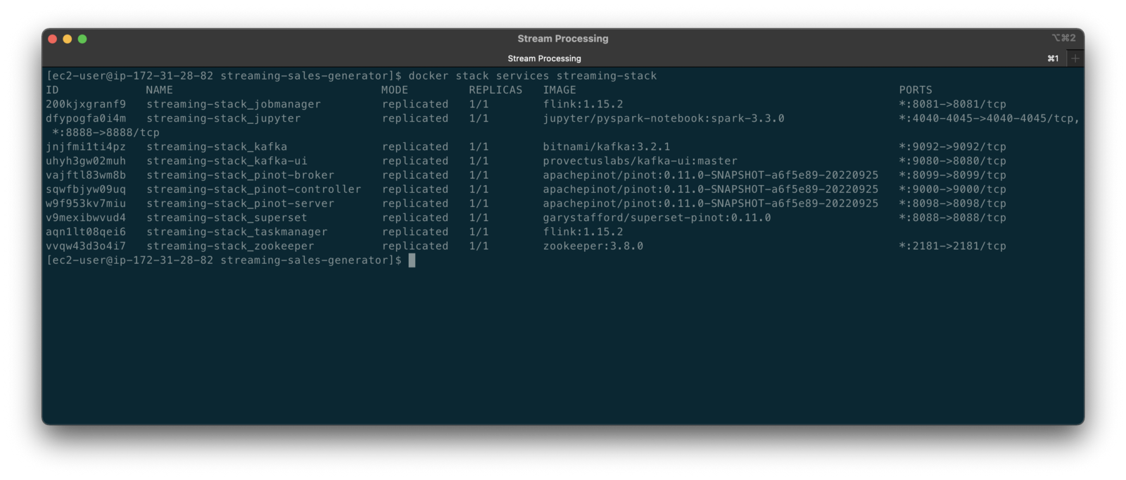
To get started, we need to replace the first streaming Docker Swarm stack, deployed in part one, with the second streaming Docker Swarm stack. The second stack contains Apache Kafka, Apache Zookeeper, Apache Flink, Apache Pinot, Apache Superset, UI for Apache Kafka, and Project Jupyter (JupyterLab).
https://programmaticponderings.wordpress.com/media/601efca17604c3a467a4200e93d7d3ff
The stack will take a few minutes to deploy fully. When complete, there should be ten containers running in the stack.
Flink Application
The Flink application has two entry classes. The first class, RunningTotals, performs an identical aggregation function as the previous KStreams demo.
The second class, JoinStreams, joins the stream of data from the demo.purchases topic and the demo.products topic, processing and combining them, in real-time, into an enriched transaction and publishing the results to a new topic, demo.purchases.enriched.
The resulting enriched purchases messages look similar to the following:
Running the Flink Job
To run the Flink application, we must first compile it into an uber JAR.
We can copy the JAR into the Flink container or upload it through the Apache Flink Dashboard, a browser-based UI. For this demonstration, we will upload it through the Apache Flink Dashboard, accessible on port 8081.
The project’s build.gradle file has preset the Main class (Flink’s Entry class) to org.example.JoinStreams. Optionally, to run the Running Totals demo, we could change the build.gradle file and recompile, or simply change Flink’s Entry class to org.example.RunningTotals.

Before running the Flink job, restart the sales generator in the background (nohup python3 ./producer.py &) to generate a new stream of data. Then start the Flink job.

To confirm the Flink application is running, we can check the contents of the new demo.purchases.enriched topic using the Kafka CLI.

Alternatively, you can use the UI for Apache Kafka, accessible on port 9080.

Demonstration #4: Apache Pinot
In the fourth and final demonstration, we will explore Apache Pinot. First, we will query the unbounded data streams from Apache Kafka, generated by both the sales generator and the Apache Flink application, using SQL. Then, we build a real-time dashboard in Apache Superset, with Apache Pinot as our datasource.

Creating Tables
According to the Apache Pinot documentation, “a table is a logical abstraction that represents a collection of related data. It is composed of columns and rows (known as documents in Pinot).” There are three types of Pinot tables: Offline, Realtime, and Hybrid. For this demonstration, we will create three Realtime tables. Realtime tables ingest data from streams — in our case, Kafka — and build segments from the consumed data. Further, according to the documentation, “each table in Pinot is associated with a Schema. A schema defines what fields are present in the table along with the data types. The schema is stored in Zookeeper, along with the table configuration.”
Below, we see the schema and config for one of the three Realtime tables, purchasesEnriched. Note how the columns are divided into three categories: Dimension, Metric, and DateTime.
To begin, copy the three Pinot Realtime table schemas and configurations from the streaming-sales-generator GitHub project into the Apache Pinot Controller container. Next, use a docker exec command to call the Pinot Command Line Interface’s (CLI) AddTable command to create the three tables: products, purchases, and purchasesEnriched.
To confirm the three tables were created correctly, use the Apache Pinot Data Explorer accessible on port 9000. Use the Tables tab in the Cluster Manager.

We can further inspect and edit the table’s config and schema from the Tables tab in the Cluster Manager.

The three tables are configured to read the unbounded stream of data from the corresponding Kafka topics: demo.products, demo.purchases, and demo.purchases.enriched.
Querying with Pinot
We can use Pinot’s Query Console to query the Realtime tables using SQL. According to the documentation, “Pinot provides a SQL interface for querying. It uses the [Apache] Calcite SQL parser to parse queries and uses MYSQL_ANSI dialect.”

With the generator still running, re-query the purchases table in the Query Console (select count(*) from purchases). You should notice the document count increasing each time you re-run the query since new messages are published to the demo.purchases topic by the sales generator.
If you do not observe the count increasing, ensure the sales generator and Flink enrichment job are running.

Table Joins?
It might seem logical to want to replicate the same multi-stream join we performed with Apache Flink in part three of the demonstration on the demo.products and demo.purchases topics. Further, we might presume to join the products and purchases realtime tables by writing a SQL statement in Pinot’s Query Console. However, according to the documentation, at the time of this post, version 0.11.0 of Pinot did not [currently] support joins or nested subqueries.
This current join limitation is why we created the Realtime table, purchasesEnriched, allowing us to query Flink’s real-time results in the demo.purchases.enriched topic. We will use both Flink and Pinot as part of our stream processing pipeline, taking advantage of each tool’s individual strengths and capabilities.
Note, according to the documentation for the latest release of Pinot on the main branch, “the latest Pinot multi-stage supports inner join, left-outer, semi-join, and nested queries out of the box. It is optimized for in-memory process and latency.” For more information on joins as part of Pinot’s new multi-stage query execution engine, read the documentation, Multi-Stage Query Engine.

demo.purchases.enriched topic in real-timeAggregations
We can perform real-time aggregations using Pinot’s rich SQL query interface. For example, like previously with Spark and Flink, we can calculate running totals for the number of items sold and the total sales for each product in real time.

We can do the same with the purchasesEnriched table, which will use the continuous stream of enriched transaction data from our Apache Flink application. With the purchasesEnriched table, we can add the product name and product category for richer results. Each time we run the query, we get real-time results based on the running sales generator and Flink enrichment job.

Query Options and Indexing
Note the reference to the Star-Tree index at the start of the SQL query shown above. Pinot provides several query options, including useStarTree (true by default).
Multiple indexing techniques are available in Pinot, including Forward Index, Inverted Index, Star-tree Index, Bloom Filter, and Range Index, among others. Each has advantages in different query scenarios. According to the documentation, by default, Pinot creates a dictionary-encoded forward index for each column.
SQL Examples
Here are a few examples of SQL queries you can try in Pinot’s Query Console:
Troubleshooting Pinot
If have issues with creating the tables or querying the real-time data, you can start by reviewing the Apache Pinot logs:
Real-time Dashboards with Apache Superset
To display the real-time stream of data produced results of our Apache Flink stream processing job and made queriable by Apache Pinot, we can use Apache Superset. Superset positions itself as “a modern data exploration and visualization platform.” Superset allows users “to explore and visualize their data, from simple line charts to highly detailed geospatial charts.”
According to the documentation, “Superset requires a Python DB-API database driver and a SQLAlchemy dialect to be installed for each datastore you want to connect to.” In the case of Apache Pinot, we can use pinotdb as the Python DB-API and SQLAlchemy dialect for Pinot. Since the existing Superset Docker container does not have pinotdb installed, I have built and published a Docker Image with the driver and deployed it as part of the second streaming stack of containers.
First, we much configure the Superset container instance. These instructions are documented as part of the Superset Docker Image repository.
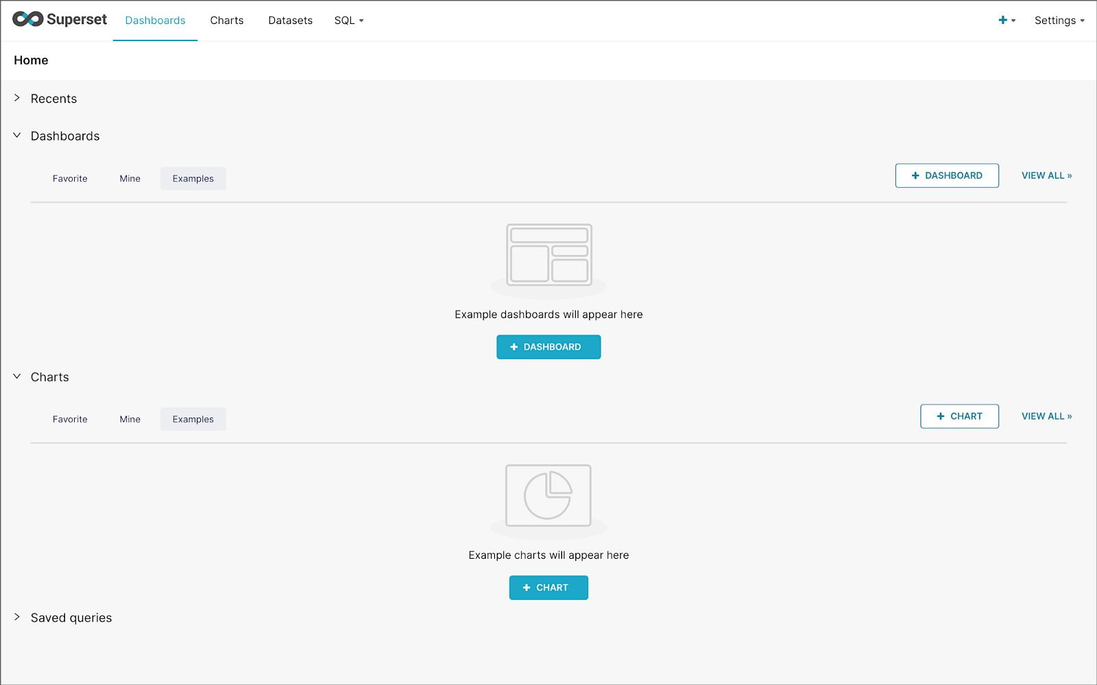
Once the configuration is complete, we can log into the Superset web-browser-based UI accessible on port 8088.
Pinot Database Connection and Dataset
Next, to connect to Pinot from Superset, we need to create a Database Connection and a Dataset.
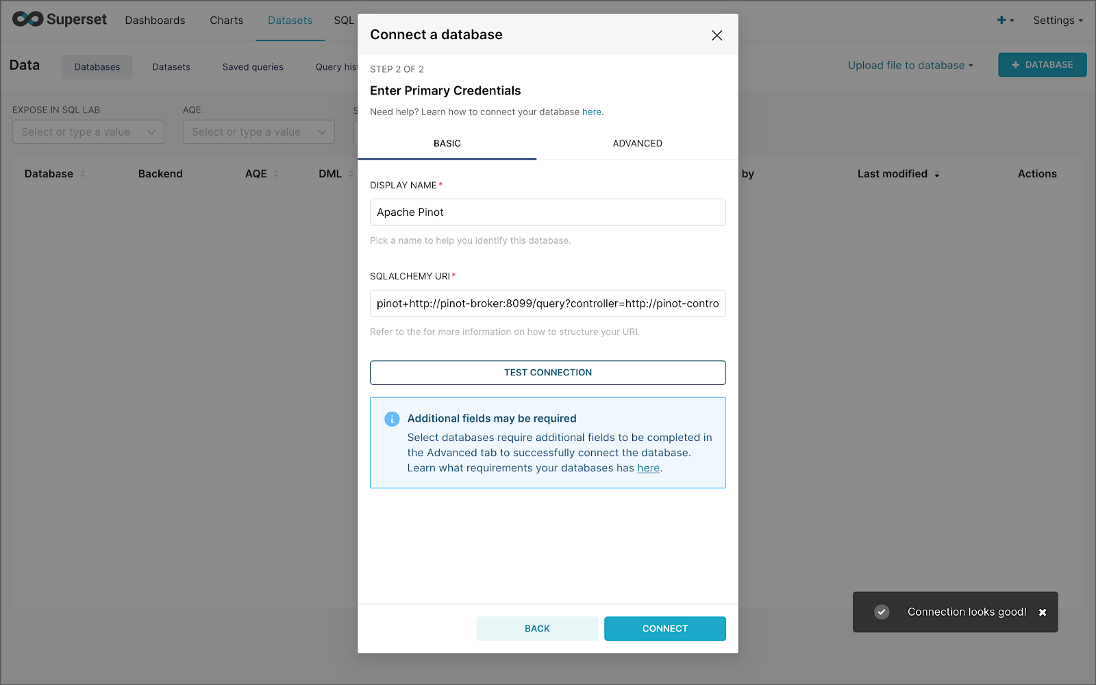
The SQLAlchemy URI is shown below. Input the URI, test your connection (‘Test Connection’), make sure it succeeds, then hit ‘Connect’.
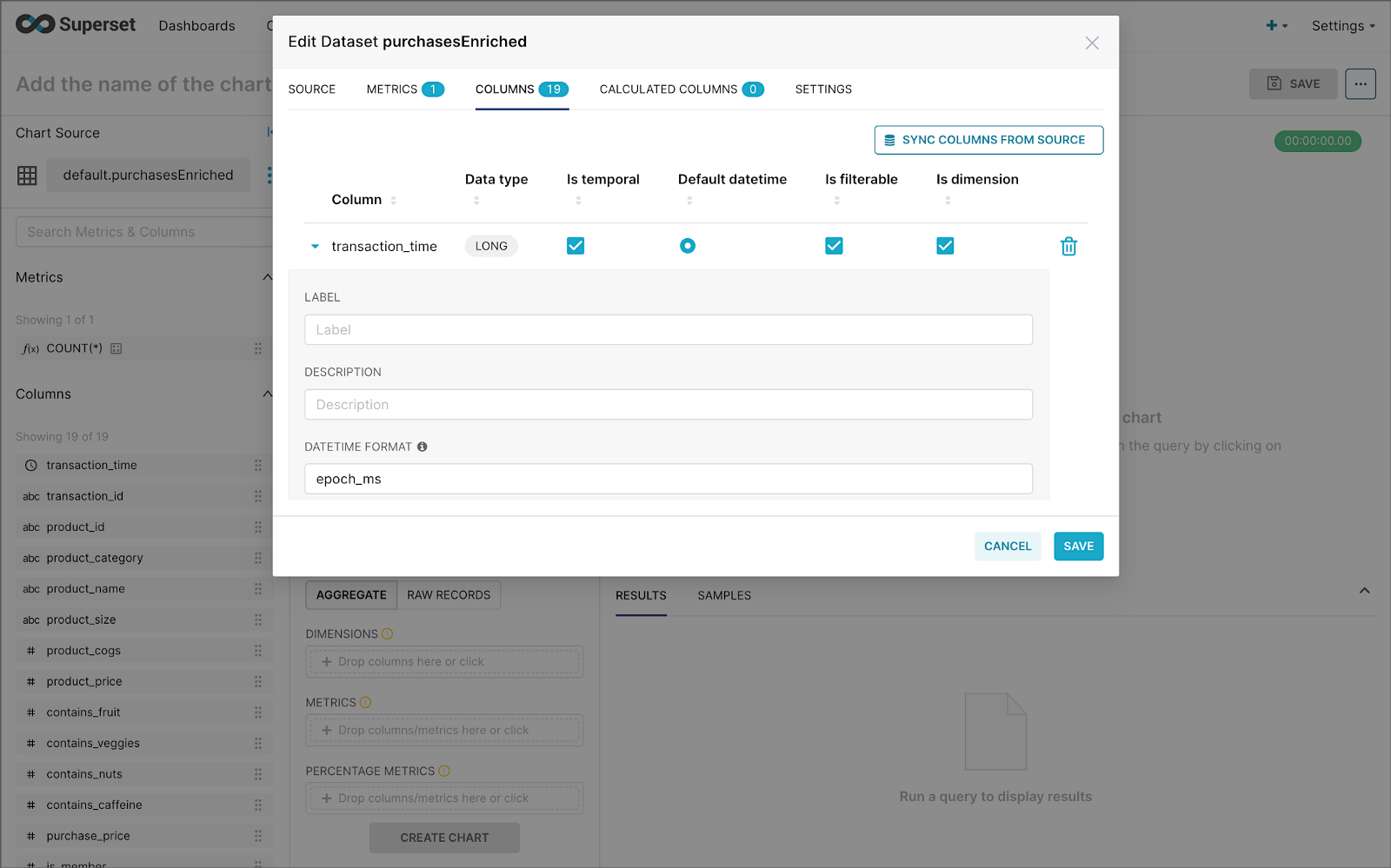
Next, create a Dataset that references the purchasesEnriched Pinot table.

purchasesEnriched Pinot tableModify the dataset’s transaction_time column. Check the is_temporal and Default datetime options. Lastly, define the DateTime format as epoch_ms.
transaction_time columnBuilding a Real-time Dashboard
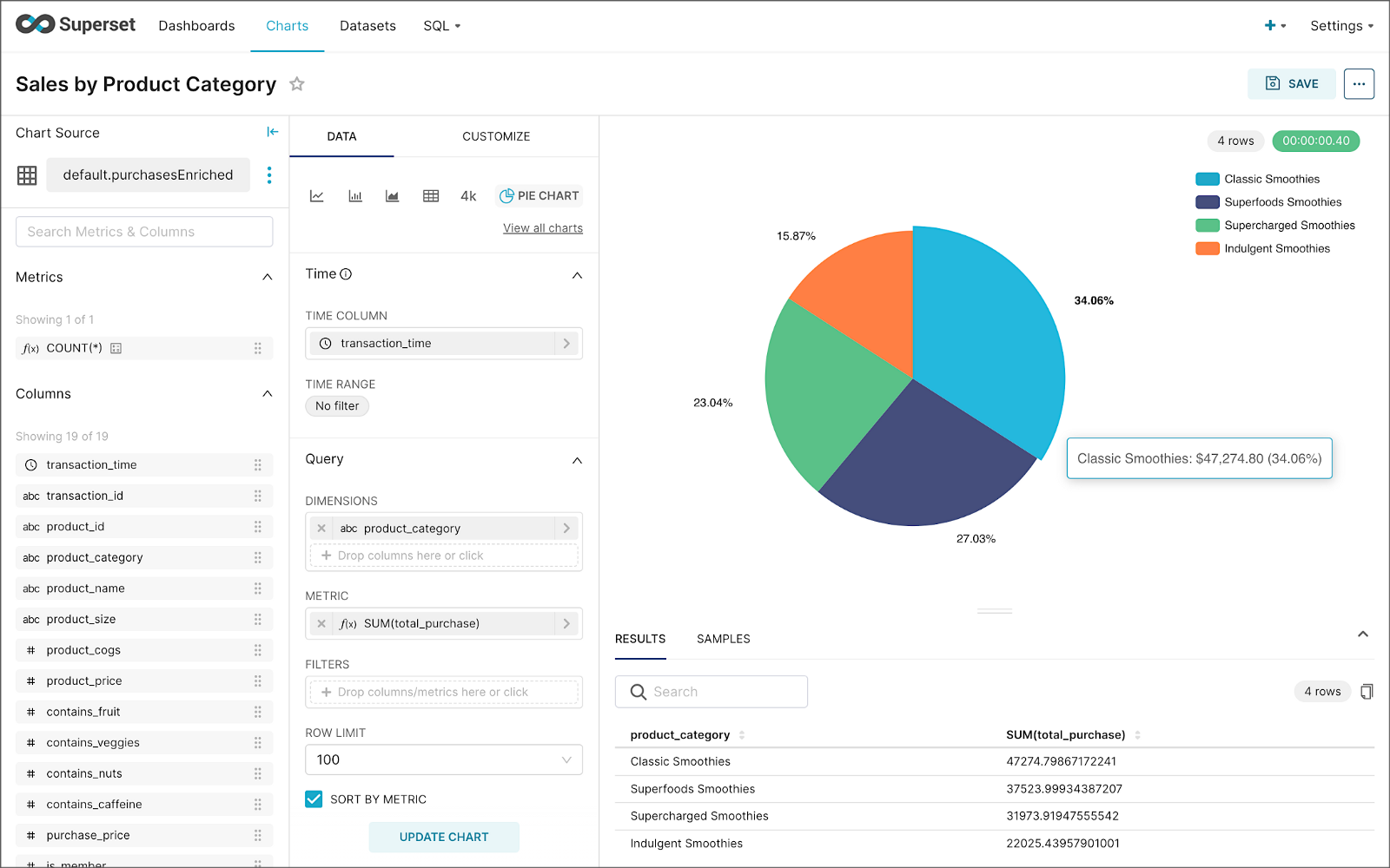
Using the new dataset, which connects Superset to the purchasesEnriched Pinot table, we can construct individual charts to be placed on a dashboard. Build a few charts to include on your dashboard.
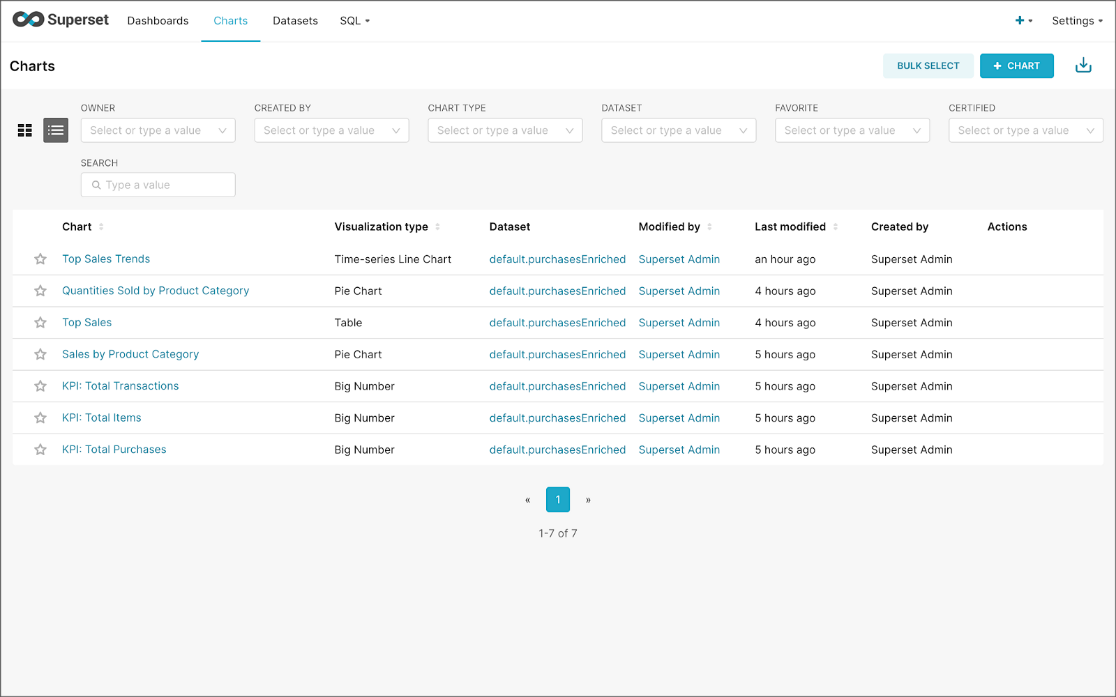
Create a new Superset dashboard and add the charts and other elements, such as headlines, dividers, and tabs.

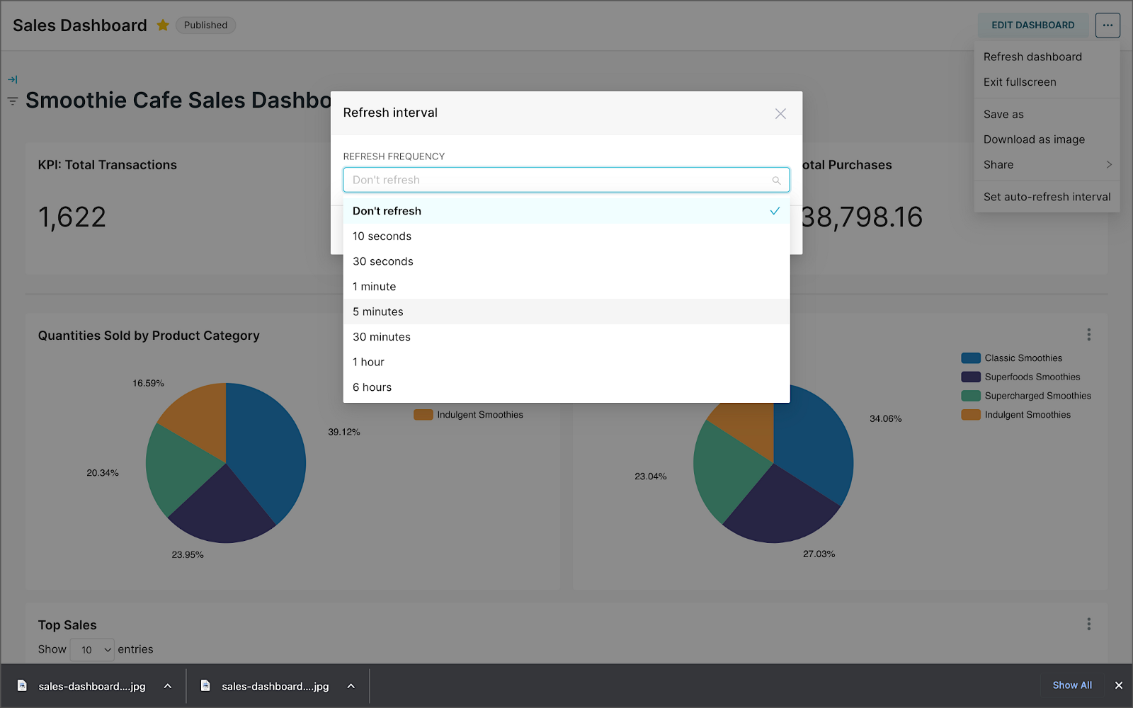
We can apply a refresh interval to the dashboard to continuously query Pinot and visualize the results in near real-time.
Conclusion
In this two-part post series, we were introduced to stream processing. We explored four popular open-source stream processing projects: Apache Spark Structured Streaming, Apache Kafka Streams, Apache Flink, and Apache Pinot. Next, we learned how we could solve similar stream processing and streaming analytics challenges using different streaming technologies. Lastly, we saw how these technologies, such as Kafka, Flink, Pinot, and Superset, could be integrated to create effective stream processing pipelines.
This blog represents my viewpoints and not of my employer, Amazon Web Services (AWS). All product names, logos, and brands are the property of their respective owners. All diagrams and illustrations are the property of the author unless otherwise noted.
Exploring Popular Open-source Stream Processing Technologies: Part 1 of 2
Posted by Gary A. Stafford in Analytics, Big Data, Java Development, Python, Software Development, SQL on September 24, 2022
A brief demonstration of Apache Spark Structured Streaming, Apache Kafka Streams, Apache Flink, and Apache Pinot with Apache Superset
Introduction
According to TechTarget, “Stream processing is a data management technique that involves ingesting a continuous data stream to quickly analyze, filter, transform or enhance the data in real-time. Once processed, the data is passed off to an application, data store, or another stream processing engine.” Confluent, a fully-managed Apache Kafka market leader, defines stream processing as “a software paradigm that ingests, processes, and manages continuous streams of data while they’re still in motion.”
Batch vs. Stream Processing
Again, according to Confluent, “Batch processing is when the processing and analysis happens on a set of data that have already been stored over a period of time.” A batch processing example might include daily retail sales data, which is aggregated and tabulated nightly after the stores close. Conversely, “streaming data processing happens as the data flows through a system. This results in analysis and reporting of events as it happens.” To use a similar example, instead of nightly batch processing, the streams of sales data are processed, aggregated, and analyzed continuously throughout the day — sales volume, buying trends, inventory levels, and marketing program performance are tracked in real time.
Bounded vs. Unbounded Data
According to Packt Publishing’s book, Learning Apache Apex, “bounded data is finite; it has a beginning and an end. Unbounded data is an ever-growing, essentially infinite data set.” Batch processing is typically performed on bounded data, whereas stream processing is most often performed on unbounded data.
Stream Processing Technologies
There are many technologies available to perform stream processing. These include proprietary custom software, commercial off-the-shelf (COTS) software, fully-managed service offerings from Software as a Service (or SaaS) providers, Cloud Solution Providers (CSP), Commercial Open Source Software (COSS) companies, and popular open-source projects from the Apache Software Foundation and Linux Foundation.
The following two-part post and forthcoming video will explore four popular open-source software (OSS) stream processing projects, including Apache Spark Structured Streaming, Apache Kafka Streams, Apache Flink, and Apache Pinot. Each of these projects has some equivalent SaaS, CSP, and COSS offerings.
This post uses the open-source projects, making it easier to follow along with the demonstration and keeping costs to a minimum. However, you could easily substitute the open-source projects for your preferred SaaS, CSP, or COSS service offerings.
Apache Spark Structured Streaming
According to the Apache Spark documentation, “Structured Streaming is a scalable and fault-tolerant stream processing engine built on the Spark SQL engine. You can express your streaming computation the same way you would express a batch computation on static data.” Further, “Structured Streaming queries are processed using a micro-batch processing engine, which processes data streams as a series of small batch jobs thereby achieving end-to-end latencies as low as 100 milliseconds and exactly-once fault-tolerance guarantees.” In the post, we will examine both batch and stream processing using a series of Apache Spark Structured Streaming jobs written in PySpark.

Apache Kafka Streams
According to the Apache Kafka documentation, “Kafka Streams [aka KStreams] is a client library for building applications and microservices, where the input and output data are stored in Kafka clusters. It combines the simplicity of writing and deploying standard Java and Scala applications on the client side with the benefits of Kafka’s server-side cluster technology.” In the post, we will examine a KStreams application written in Java that performs stream processing and incremental aggregation.

Apache Flink
According to the Apache Flink documentation, “Apache Flink is a framework and distributed processing engine for stateful computations over unbounded and bounded data streams. Flink has been designed to run in all common cluster environments, perform computations at in-memory speed and at any scale.” Further, “Apache Flink excels at processing unbounded and bounded data sets. Precise control of time and state enables Flink’s runtime to run any kind of application on unbounded streams. Bounded streams are internally processed by algorithms and data structures that are specifically designed for fixed-sized data sets, yielding excellent performance.” In the post, we will examine a Flink application written in Java, which performs stream processing, incremental aggregation, and multi-stream joins.

Apache Pinot
According to Apache Pinot’s documentation, “Pinot is a real-time distributed OLAP datastore, purpose-built to provide ultra-low-latency analytics, even at extremely high throughput. It can ingest directly from streaming data sources — such as Apache Kafka and Amazon Kinesis — and make the events available for querying instantly. It can also ingest from batch data sources such as Hadoop HDFS, Amazon S3, Azure ADLS, and Google Cloud Storage.” In the post, we will query the unbounded data streams from Apache Kafka, generated by Apache Flink, using SQL.

Streaming Data Source
We must first find a good unbounded data source to explore or demonstrate these streaming technologies. Ideally, the streaming data source should be complex enough to allow multiple types of analyses and visualize different aspects with Business Intelligence (BI) and dashboarding tools. Additionally, the streaming data source should possess a degree of consistency and predictability while displaying a reasonable level of variability and randomness.
To this end, we will use the open-source Streaming Synthetic Sales Data Generator project, which I have developed and made available on GitHub. This project’s highly-configurable, Python-based, synthetic data generator generates an unbounded stream of product listings, sales transactions, and inventory restocking activities to a series of Apache Kafka topics.

Source Code
All the source code demonstrated in this post is open source and available on GitHub. There are three separate GitHub projects:
Docker
To make it easier to follow along with the demonstration, we will use Docker Swarm to provision the streaming tools. Alternatively, you could use Kubernetes (e.g., creating a Helm chart) or your preferred CSP or SaaS managed services. Nothing in this demonstration requires you to use a paid service.
The two Docker Swarm stacks are located in the Streaming Synthetic Sales Data Generator project:
- Streaming Stack — Part 1: Apache Kafka, Apache Zookeeper, Apache Spark, UI for Apache Kafka, and the KStreams application
- Streaming Stack — Part 2: Apache Kafka, Apache Zookeeper, Apache Flink, Apache Pinot, Apache Superset, UI for Apache Kafka, and Project Jupyter (JupyterLab).*
* the Jupyter container can be used as an alternative to the Spark container for running PySpark jobs (follow the same steps as for Spark, below)
Demonstration #1: Apache Spark
In the first of four demonstrations, we will examine two Apache Spark Structured Streaming jobs, written in PySpark, demonstrating both batch processing (spark_batch_kafka.py) and stream processing (spark_streaming_kafka.py). We will read from a single stream of data from a Kafka topic, demo.purchases, and write to the console.

Deploying the Streaming Stack
To get started, deploy the first streaming Docker Swarm stack containing the Apache Kafka, Apache Zookeeper, Apache Spark, UI for Apache Kafka, and the KStreams application containers.
The stack will take a few minutes to deploy fully. When complete, there should be a total of six containers running in the stack.

Sales Generator
Before starting the streaming data generator, confirm or modify the configuration/configuration.ini. Three configuration items, in particular, will determine how long the streaming data generator runs and how much data it produces. We will set the timing of transaction events to be generated relatively rapidly for test purposes. We will also set the number of events high enough to give us time to explore the Spark jobs. Using the below settings, the generator should run for an average of approximately 50–60 minutes: (((5 sec + 2 sec)/2)*1000 transactions)/60 sec=~58 min on average. You can run the generator again if necessary or increase the number of transactions.
Start the streaming data generator as a background service:
The streaming data generator will start writing data to three Apache Kafka topics: demo.products, demo.purchases, and demo.inventories. We can view these topics and their messages by logging into the Apache Kafka container and using the Kafka CLI:
Below, we see a few sample messages from the demo.purchases topic:

demo.purchases topicAlternatively, you can use the UI for Apache Kafka, accessible on port 9080.

demo.purchases topic in the UI for Apache Kafka
demo.purchases topic using the UI for Apache KafkaPrepare Spark
Next, prepare the Spark container to run the Spark jobs:
Running the Spark Jobs
Next, copy the jobs from the project to the Spark container, then exec back into the container:
Batch Processing with Spark
The first Spark job, spark_batch_kafka.py, aggregates the number of items sold and the total sales for each product, based on existing messages consumed from the demo.purchases topic. We use the PySpark DataFrame class’s read() and write() methods in the first example, reading from Kafka and writing to the console. We could just as easily write the results back to Kafka.
The batch processing job sorts the results and outputs the top 25 items by total sales to the console. The job should run to completion and exit successfully.

To run the batch Spark job, use the following commands:
Stream Processing with Spark
The stream processing Spark job, spark_streaming_kafka.py, also aggregates the number of items sold and the total sales for each item, based on messages consumed from the demo.purchases topic. However, as shown in the code snippet below, this job continuously aggregates the stream of data from Kafka, displaying the top ten product totals within an arbitrary ten-minute sliding window, with a five-minute overlap, and updates output every minute to the console. We use the PySpark DataFrame class’s readStream() and writeStream() methods as opposed to the batch-oriented read() and write() methods in the first example.
Shorter event-time windows are easier for demonstrations — in Production, hourly, daily, weekly, or monthly windows are more typical for sales analysis.

To run the stream processing Spark job, use the following commands:
We could just as easily calculate running totals for the stream of sales data versus aggregations over a sliding event-time window (example job included in project).

Be sure to kill the stream processing Spark jobs when you are done, or they will continue to run, awaiting more data.
Demonstration #2: Apache Kafka Streams
Next, we will examine Apache Kafka Streams (aka KStreams). For this part of the post, we will also use the second of the three GitHub repository projects, kstreams-kafka-demo. The project contains a KStreams application written in Java that performs stream processing and incremental aggregation.
KStreams Application
The KStreams application continuously consumes the stream of messages from the demo.purchases Kafka topic (source) using an instance of the StreamBuilder() class. It then aggregates the number of items sold and the total sales for each item, maintaining running totals, which are then streamed to a new demo.running.totals topic (sink). All of this using an instance of the KafkaStreams() Kafka client class.
Running the Application
We have at least three choices to run the KStreams application for this demonstration: 1) running locally from our IDE, 2) a compiled JAR run locally from the command line, or 3) a compiled JAR copied into a Docker image, which is deployed as part of the Swarm stack. You can choose any of the options.
Compiling and running the KStreams application locally
We will continue to use the same streaming Docker Swarm stack used for the Apache Spark demonstration. I have already compiled a single uber JAR file using OpenJDK 17 and Gradle from the project’s source code. I then created and published a Docker image, which is already part of the running stack.
Since we ran the sales generator earlier for the Spark demonstration, there is existing data in the demo.purchases topic. Re-run the sales generator (nohup python3 ./producer.py &) to generate a new stream of data. View the results of the KStreams application, which has been running since the stack was deployed using the Kafka CLI or UI for Apache Kafka:
Below, in the top terminal window, we see the output from the KStreams application. Using KStream’s peek() method, the application outputs Purchase and Total instances to the console as they are processed and written to Kafka. In the lower terminal window, we see new messages being published as a continuous stream to output topic, demo.running.totals.

Part Two
In part two of this two-part post, we continue our exploration of the four popular open-source stream processing projects. We will cover Apache Flink and Apache Pinot. In addition, we will incorporate Apache Superset into the demonstration, building a real-time dashboard to visualize the results of our stream processing.
This blog represents my viewpoints and not of my employer, Amazon Web Services (AWS). All product names, logos, and brands are the property of their respective owners. All diagrams and illustrations are the property of the author unless otherwise noted.
Capturing Data Analytics Workflows and System Requirements
Posted by Gary A. Stafford in Analytics, Big Data, Technology Consulting on January 21, 2022
Implement an effective, consistent, and repeatable strategy for documenting data analytics workflows and capturing system requirements
“Data analytics applications involve more than just analyzing data, particularly on advanced analytics projects. Much of the required work takes place upfront, in collecting, integrating, and preparing data and then developing, testing, and revising analytical models to ensure that they produce accurate results. In addition to data scientists and other data analysts, analytics teams often include data engineers, who create data pipelines and help prepare data sets for analysis.” — TechTarget
Introduction
Successful consultants, project managers, and product owners use well-proven and systematic approaches to achieve desired outcomes, including successful customer engagements, project results, and product and service launches. Modern data stacks and analytics workflows are increasingly complex. This technology-agnostic discovery process aims to help an organization efficiently and repeatably capture a concise record of existing analytics workflows, business and technical goals and constraints, and measures of success. If applicable, the discovery process is also used to compile and clarify requirements for new data analytics workflows.

Analytics Workflow Stages
There are many patterns organizations use to delineate the stages of their analytics workflows. This process utilizes six stages of a typical analytics workflow:
- Generate: All the ways data is generated and the systems of record where it is stored or originates from, also referred to as data ingress
- Collect: All the ways data is collected or ingested
- Prepare: All the ways data is transformed, including ETL, ELT, reverse ETL, and ML
- Store: All the ways data is stored, organized, and secured for analytics purposes
- Analyze: All the ways data is analyzed
- Deliver: All the ways data is delivered and how it is consumed, also referred to as data egress or data products
The precise nomenclature is not critical to this process as long as all major functionality is considered.
The Process
The discovery process starts by working backward. It first identifies existing goals and desired outcomes. It then identifies existing and anticipated future constraints. Next, it breaks down the current analytics workflows, examining the four stages of collect, prepare, store, and analyze, the steps required to get from data sources to deliverables. Finally, it captures the inputs and the outputs for the workflows and the data producers and consumers.
Collect, prepare, store, and analyze — the steps required to get from data sources to deliverables.
Specifically, the process identifies and documents the following:
- Business and technical goals and desired outcomes
- Business and technical constraints also referred to as limitations or restrictions
- Analytics workflows: tools, techniques, procedures, and organizational structure
- Outputs also referred to as deliverables, required to achieve desired outcomes
- Inputs, also referred to as data sources, required to achieve desired outcomes
- Data producers and consumers
- Measures of success
- Recommended next steps
Outcomes
Capture business and technical goals and desired outcomes driving the necessity to rearchitect current analytics processes. For example:
- Re-architect analytics processes to modernize, reduce complexity, or add new capabilities
- Reduce or control costs
- Increase performance, scalability, speed
- Migrate on-premises workloads, workflows, processes to the Cloud
- Migrate from one cloud provider or SaaS provider to another
- Move away from proprietary software products to open source software (OSS) or commercial open source software (COSS)
- Migrate away from custom-built software to commercial off-the-shelf (COTS), OSS, or COSS solutions
- Integrate DevOps, GitOps, DataOps, or MLOps practices
- Integrate on-premises, multi-cloud, and SaaS-based hybrid architectures
- Develop new analytics product or service offerings
- Standardize analytics processes
- Leverage the data for AI and ML purposes
- Provide stakeholders with a real-time business KPIs dashboard
- Construct a data lake, data warehouse, data lakehouse, or data mesh
If migration is involved, review the 6 R’s of Cloud Migration: Rehost, Replatform, Repurchase, Refactor, Retain, or Retire.
Constraints
Identify the existing and potential future business and technical constraints that impact analytics workflows. For example:
- Budgets
- Cost attribution
- Timelines
- Access to skilled resources
- Internal and external regulatory requirements, such as HIPAA, SOC2, FedRAMP, GDPR, PCI DSS, CCPA, and FISMA
- Business Continuity and Disaster Recovery (BCDR) requirements
- Architecture Review Board (ARB), Center of Excellence (CoE), Change Advisory Board (CAB), and Release Management standards and guidelines
- Data residency and data sovereignty requirements
- Security policies
- Service Level Agreements (SLAs); see ‘Measures of Success’ section
- Existing vendor, partner, cloud-provider, and SaaS relationships
- Existing licensing and contractual obligations
- Deprecated code dependencies and other technical debt
- Must-keep aspects of existing processes
- Build versus buy propensity
- Proprietary versus open source software propensity
- Insourcing versus outsourcing propensity
- Managed, hosted, SaaS versus self-managed software propensity

Analytics Workflows
Capture analytics workflows using the four stages of collect, prepare, store, and analyze, as a way to organize the discussion:
- High- and low-level architecture, process flow diagrams, sequence diagrams
- Recent architectural assessments such as reviews based on the AWS Data Analytics Lens, AWS Well-Architected Framework, Microsoft Azure Well-Architected Framework, or Google Cloud Architecture Framework
- Analytics tools, including hardware and commercial, custom, and open-source software
- Security policies, processes, standards, and technologies
- Observability, logging, monitoring, alerting, and notification
- Teams, including roles, responsibilities, and skillsets
- Partners, including consultants, vendors, SaaS providers, and Managed Service Providers (MSP)
- SDLC environments, such as Local, Sandbox, Development, Testing, Staging, Production, and Disaster Recovery (DR)
- Business Continuity Planning (BCP) policies, processes, standards, and technologies
- Primary analytics programming languages
- External system dependencies
- DataOps, MLOps, DevOps, CI/CD, SCM/VCS, and Infrastructure-as-Code (IaC) automation policies, processes, standards, and technologies
- Data governance and data lineage policies, processes, standards, and technologies
- Data quality (or data assurance) policies, processes, standards, technologies, and testing methodologies
- Data anomaly detection policies, processes, standards, and technologies
- Intellectual property (IP), the ‘secret sauce’ that differentiates the organization’s processes and provides a competitive advantage, such as ML models, proprietary algorithms, datasets, highly specialized knowledge, and patents
- Overall effectiveness and customer satisfaction with existing analytics platform (document sources of customer feedback)
- Known deficiencies with current analytics processes

Outputs
Identify the deliverables required to meet the desired outcomes. For example, prepare and provide data for:
- Data analytics purposes
- Business Intelligence (BI), visualizations, and dashboards
- Machine Learning (ML) and Artificial Intelligence (AI)
- Data exports and data feeds, such as Excel or CSV-format files
- Hosted datasets for external or internal consumption
- Data APIs for external or internal consumption
- Documentation, Data API guides, data dictionaries, example code such as Notebooks
- SaaS-based product offering

Inputs
Capture sources of data that are required to produce the outputs. For example:
- Batch sources such as flat files from legacy systems, third-party providers, and enterprise platforms
- Streaming sources such as message queues, change data capture (CDC), IoT device telemetry, operational metrics, real time logs, clickstream data, connected devices, mobile, and gaming feeds
- Databases, including relational, NoSQL, key-value, document, in-memory, graph, time series, and wide column (OLTP data stores)
- Data warehouses (OLAP data stores)
- Data lakes
- API endpoints
- Internal, public, and licensed datasets
Use the 5 V’s of big data to dive deep into each data source: Volume, Velocity, Variety, Veracity (or Validity), and Value.

Data Producers and Consumers
Capture all producers and consumers of data:
- Data producers
- Data consumers
- Data access patterns
- Data usage patterns
- Consumer and producer requirements and constraints

Measures of Success
Identify how success is measured for the analytics workflows and by whom. For example:
- Key Performance Indicators (KPIs)
- Service Level Agreements (SLAs)
- Customer Satisfaction Score (CSAT)
- Net Promoter Score (NPS)
- SaaS growth metrics: churn, activation rate, MRR, ARR, CAC, CLV, expansion revenue (source: appcues.com)
- Data quality guarantees
- How are measurements determined, calculated, and weighted?
- What are the business and technical actions resulting from missed measures of success?
Results
The immediate artifact of the data analytics discovery process is a clear and concise document that captures all feedback and inputs. In addition, the document contains all customer-supplied artifacts, such as architectural and process flow diagrams. The document should be thoroughly reviewed for accuracy and completeness by the process participants. This artifact serves as a record of current data analytics workflows and a basis for making workflow improvement recommendations or architecting new workflows.
This blog represents my own viewpoints and not of my employer, Amazon Web Services (AWS). All product names, logos, and brands are the property of their respective owners.
Running Spark Jobs on Amazon EMR with Apache Airflow: Using the new Amazon Managed Workflows for Apache Airflow (Amazon MWAA) Service on AWS
Posted by Gary A. Stafford in AWS, Bash Scripting, Big Data, Build Automation, Cloud, DevOps, Python, Software Development on December 24, 2020
Introduction
In the first post of this series, we explored several ways to run PySpark applications on Amazon EMR using AWS services, including AWS CloudFormation, AWS Step Functions, and the AWS SDK for Python. This second post in the series will examine running Spark jobs on Amazon EMR using the recently announced Amazon Managed Workflows for Apache Airflow (Amazon MWAA) service.
Amazon EMR
According to AWS, Amazon Elastic MapReduce (Amazon EMR) is a Cloud-based big data platform for processing vast amounts of data using common open-source tools such as Apache Spark, Hive, HBase, Flink, Hudi, and Zeppelin, Jupyter, and Presto. Using Amazon EMR, data analysts, engineers, and scientists are free to explore, process, and visualize data. EMR takes care of provisioning, configuring, and tuning the underlying compute clusters, allowing you to focus on running analytics.

Users interact with EMR in a variety of ways, depending on their specific requirements. For example, you might create a transient EMR cluster, execute a series of data analytics jobs using Spark, Hive, or Presto, and immediately terminate the cluster upon job completion. You only pay for the time the cluster is up and running. Alternatively, for time-critical workloads or continuously high volumes of jobs, you could choose to create one or more persistent, highly available EMR clusters. These clusters automatically scale compute resources horizontally, including the use of EC2 Spot instances, to meet processing demands, maximizing performance and cost-efficiency.
AWS currently offers 5.x and 6.x versions of Amazon EMR. Each major and minor release of Amazon EMR offers incremental versions of nearly 25 different, popular open-source big-data applications to choose from, which Amazon EMR will install and configure when the cluster is created. The latest Amazon EMR releases are Amazon EMR Release 6.2.0 and Amazon EMR Release 5.32.0.
Amazon MWAA
Apache Airflow is a popular open-source platform designed to schedule and monitor workflows. According to Wikipedia, Airflow was created at Airbnb in 2014 to manage the company’s increasingly complex workflows. From the beginning, the project was made open source, becoming an Apache Incubator project in 2016 and a top-level Apache Software Foundation project (TLP) in 2019.
Many organizations build, manage, and maintain Apache Airflow on AWS using compute services such as Amazon EC2 or Amazon EKS. Amazon recently announced Amazon Managed Workflows for Apache Airflow (Amazon MWAA). With the announcement of Amazon MWAA in November 2020, AWS customers can now focus on developing workflow automation, while leaving the management of Airflow to AWS. Amazon MWAA can be used as an alternative to AWS Step Functions for workflow automation on AWS.

Apache recently announced the release of Airflow 2.0.0 on December 17, 2020. The latest 1.x version of Airflow is 1.10.14, released December 12, 2020. However, at the time of this post, Amazon MWAA was running Airflow 1.10.12, released August 25, 2020. Ensure that when you are developing workflows for Amazon MWAA, you are using the correct Apache Airflow 1.10.12 documentation.
The Amazon MWAA service is available using the AWS Management Console, as well as the Amazon MWAA API using the latest versions of the AWS SDK and AWS CLI.
Airflow has a mechanism that allows you to expand its functionality and integrate with other systems. Given its integration capabilities, Airflow has extensive support for AWS, including Amazon EMR, Amazon S3, AWS Batch, Amazon RedShift, Amazon DynamoDB, AWS Lambda, Amazon Kinesis, and Amazon SageMaker. Outside of support for Amazon S3, most AWS integrations can be found in the Hooks, Secrets, Sensors, and Operators of Airflow codebase’s contrib section.
Getting Started
Source Code
Using this git clone command, download a copy of this post’s GitHub repository to your local environment.
git clone --branch main --single-branch --depth 1 --no-tags \
    https://github.com/garystafford/aws-airflow-demo.git
Preliminary Steps
This post assumes the reader has completed the demonstration in the previous post, Running PySpark Applications on Amazon EMR Methods for Interacting with PySpark on Amazon Elastic MapReduce. This post will re-use many of the last post’s AWS resources, including the EMR VPC, Subnets, Security Groups, AWS Glue Data Catalog, Amazon S3 buckets, EMR Roles, EC2 key pair, AWS Systems Manager Parameter Store parameters, PySpark applications, and Kaggle datasets.
Configuring Amazon MWAA
The easiest way to create a new MWAA Environment is through the AWS Management Console. I strongly suggest that you review the pricing for Amazon MWAA before continuing. The service can be quite costly to operate, even when idle, with the smallest Environment class potentially running into the hundreds of dollars per month.

Using the Console, create a new Amazon MWAA Environment. The Amazon MWAA interface will walk you through the creation process. Note the current ‘Airflow version’, 1.10.12.

Amazon MWAA requires an Amazon S3 bucket to store Airflow assets. Create a new Amazon S3 bucket. According to the documentation, the bucket must start with the prefix airflow-. You must also enable Bucket Versioning on the bucket. Specify a dags folder within the bucket to store Airflow’s Directed Acyclic Graphs (DAG). You can leave the next two options blank since we have no additional Airflow plugins or additional Python packages to install.

With Amazon MWAA, your data is secure by default as workloads run within their own Amazon Virtual Private Cloud (Amazon VPC). As part of the MWAA Environment creation process, you are given the option to have AWS create an MWAA VPC CloudFormation stack.

For this demonstration, choose to have MWAA create a new VPC and associated networking resources.

The MWAA CloudFormation stack contains approximately 22 AWS resources, including a VPC, a pair of public and private subnets, route tables, an Internet Gateway, two NAT Gateways, and associated Elastic IPs (EIP). See the MWAA documentation for more details.


As part of the Amazon MWAA Networking configuration, you must decide if you want web access to Airflow to be public or private. The details of the network configuration can be found in the MWAA documentation. I am choosing public webserver access for this demonstration, but the recommended choice is private for greater security. With the public option, AWS still requires IAM authentication to sign in to the AWS Management Console in order to access the Airflow UI.
You must select an existing VPC Security Group or have MWAA create a new one. For this demonstration, choose to have MWAA create a Security Group for you.
Lastly, select an appropriately-sized Environment class for Airflow based on the scale of your needs. The mw1.small class will be sufficient for this demonstration.

Finally, for Permissions, you must select an existing Airflow execution service role or create a new role. For this demonstration, create a new Airflow service role. We will later add additional permissions.

Airflow Execution Role
As part of this demonstration, we will be using Airflow to run Spark jobs on EMR (EMR Steps). To allow Airflow to interact with EMR, we must increase the new Airflow execution role’s default permissions. Additional permissions include allowing the new Airflow role to assume the EMR roles using iam:PassRole. For this demonstration, we will include the two default EMR Service and JobFlow roles, EMR_DefaultRole and EMR_EC2_DefaultRole. We will also include the corresponding custom EMR roles created in the previous post, EMR_DemoRole and EMR_EC2_DemoRole. For this demonstration, the Airflow service role also requires three specific EMR permissions as shown below. Later in the post, Airflow will also read files from S3, which requires s3:GetObject permission.
Create a new policy by importing the project’s JSON file, iam_policy/airflow_emr_policy.json, and attach the new policy to the Airflow service role. Be sure to update the AWS Account ID in the file with your own Account ID.
The Airflow service role, created by MWAA, is shown below with the new policy attached.

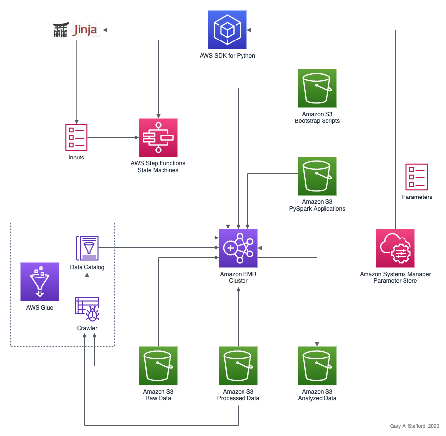
Final Architecture
Below is the final high-level architecture for the post’s demonstration. The diagram shows the approximate route of a DAG Run request, in red. The diagram includes an optional S3 Gateway VPC endpoint, not detailed in the post, but recommended for additional security. According to AWS, a VPC endpoint enables you to privately connect your VPC to supported AWS services and VPC endpoint services powered by AWS PrivateLink without requiring an internet gateway. In this case a private connection between the MWAA VPC and Amazon S3. It is also possible to create an EMR Interface VPC Endpoint to securely route traffic directly to EMR from MWAA, instead of connecting over the Internet.

Amazon MWAA Environment
The new MWAA Environment will include a link to the Airflow UI.

Airflow UI
Using the supplied link, you should be able to access the Airflow UI using your web browser.

Our First DAG
The Amazon MWAA documentation includes an example DAG, which contains one of several sample programs, SparkPi, which comes with Spark. I have created a similar DAG that is included in the GitHub project, dags/emr_steps_demo.py. The DAG will create a minimally-sized single-node EMR cluster with no Core or Task nodes. The DAG will then use that cluster to submit the calculate_pi job to Spark. Once the job is complete, the DAG will terminate the EMR cluster.
Upload the DAG to the Airflow S3 bucket’s dags directory. Substitute your Airflow S3 bucket name in the AWS CLI command below, then run it from the project’s root.
aws s3 cp dags/spark_pi_example.py \
    s3://<your_airflow_bucket_name>/dags/
The DAG, spark_pi_example, should automatically appear in the Airflow UI. Click on ‘Trigger DAG’ to create a new EMR cluster and start the Spark job.

The DAG has no optional configuration to input as JSON. Select ‘Trigger’ to submit the job, as shown below.

The DAG should complete all three tasks successfully, as shown in the DAG’s ‘Graph View’ tab below.

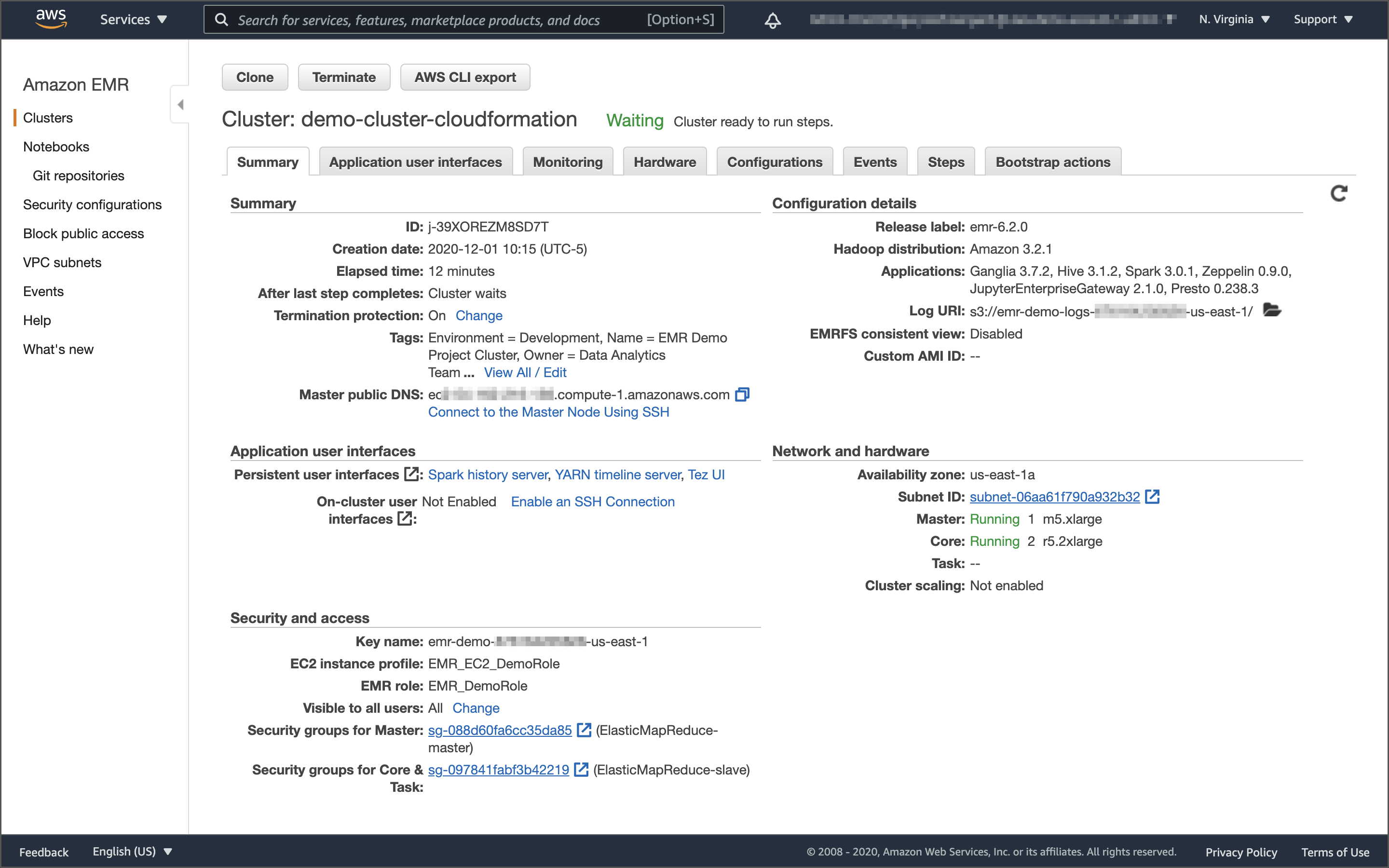
Switching to the EMR Console, you should see the single-node EMR cluster being created.

On the ‘Steps’ tab, you should see that the ‘calculate_pi’ Spark job has been submitted and is waiting for the cluster to be ready to be run.

Triggering DAGs Programmatically
The Amazon MWAA service is available using the AWS Management Console, as well as the Amazon MWAA API using the latest versions of the AWS SDK and AWS CLI. To automate the DAG Run, we could use the AWS CLI and invoke the Airflow CLI via an endpoint on the Apache Airflow Webserver. The Amazon MWAA documentation and Airflow’s CLI documentation explains how.
Below is an example of triggering the spark_pi_example DAG programmatically using Airflow’s trigger_dag CLI command. You will need to replace the WEB_SERVER_HOSTNAME variable with your own Airflow Web Server’s hostname. The ENVIROMENT_NAME variable assumes only one MWAA environment is returned by jq.
Analytics Job with Airflow
Next, we will submit an actual analytics job to EMR. If you recall from the previous post, we had four different analytics PySpark applications, which performed analyses on the three Kaggle datasets. For the next DAG, we will run a Spark job that executes the bakery_sales_ssm.py PySpark application. This job should already exist in the processed data S3 bucket.
The DAG, dags/bakery_sales.py, creates an EMR cluster identical to the EMR cluster created with the run_job_flow.py Python script in the previous post. All EMR configuration options available when using AWS Step Functions are available with Airflow’s airflow.contrib.operators and airflow.contrib.sensors packages for EMR.
Airflow leverages Jinja Templating and provides the pipeline author with a set of built-in parameters and macros. The Bakery Sales DAG contains eleven Jinja template variables. Seven variables will be configured in the Airflow UI by importing a JSON file into the ‘Admin’ ⇨ ‘Variables’ tab. These template variables are prefixed with var.value in the DAG. The other three variables will be passed as a DAG Run configuration as a JSON blob, similar to the previous DAG example. These template variables are prefixed with dag_run.conf.
Import Variables into Airflow UI
First, to import the required variables, change the values in the project’s airflow_variables/admin_variables_bakery.json file. You will need to update the values for bootstrap_bucket, emr_ec2_key_pair, logs_bucket, and work_bucket. The three S3 buckets should all exist from the previous post.
Next, import the variables file from the ‘Admin’ ⇨ ‘Variables’ tab of the Airflow UI.

Upload the DAG, dags/bakery_sales.py, to the Airflow S3 bucket, similar to the first DAG.
aws s3 cp dags/bakery_sales.py \
    s3://<your_airflow_bucket_name>/dags/
The second DAG, bakery_sales, should automatically appear in the Airflow UI. Click on ‘Trigger DAG’ to create a new EMR cluster and start the Spark job.

Input the three required parameters in the ‘Trigger DAG’ interface, used to pass the DAG Run configuration, and select ‘Trigger’. A sample of the JSON blob can be found in the project, airflow_variables/dag_run.conf_bakery.json.
{
    "airflow_email": "analytics_team@example.com",
    "email_on_failure": false,
    "email_on_retry": false
}
This is just for demonstration purposes. To send and receive emails, you will need to configure Airflow.

Switching to the EMR Console, you should see the ‘Bakery Sales’ Spark job in the ‘Steps’ tab.

Multi-Step DAG
In our last example, we will use a single DAG to run four Spark jobs in parallel. The Spark job arguments (EmrAddStepsOperator steps parameter) will be loaded from an external JSON file residing in Amazon S3, instead of defined in the DAG, as in the previous two DAG examples. Additionally, the EMR cluster specifications (EmrCreateJobFlowOperator job_flow_overrides parameter) will also be loaded from an external JSON file. Using this method, we decouple the EMR provisioning and job details from the DAG. DataOps or DevOps Engineers might manage the EMR cluster specifications as code, while Data Analysts manage the Spark job arguments, separately. A third team might manage the DAG itself.
We still maintain the variables in the JSON files. The DAG will read the JSON file-based configuration into the tasks as JSON blobs, then replace the Jinja template variables (expressions) in the DAG with variable values defined in Airflow or input as parameters when the DAG is triggered.
Below we see a snippet of two of the four Spark submit-job job definitions (steps), which have been moved to a separate JSON file, emr_steps/emr_steps.json.
Below are the EMR cluster specifications (job_flow_overrides), which have been moved to a separate JSON file, job_flow_overrides/job_flow_overrides.json.
Decoupling the configurations reduces the DAG from well over 200 lines of code to less than 75 lines. Note lines 56 and 63 of the DAG below. Instead of referencing a local object variable, the parameters now reference the function, get_objects(key, bucket_name), which loads the JSON.
This time, we need to upload three files to S3, the DAG to the Airflow S3 bucket, and the two JSON files to the EMR Work S3 bucket. Change the bucket names to match your environment, then run the three AWS CLI commands shown below.
aws s3 cp emr_steps/emr_steps.json \
    s3://emr-demo-work-123412341234-us-east-1/emr_steps/
aws s3 cp job_flow_overrides/job_flow_overrides.json \
    s3://emr-demo-work-123412341234-us-east-1/job_flow_overrides/
aws s3 cp dags/multiple_steps.py \
    s3://airflow-123412341234-us-east-1/dags/
The second DAG, multiple_steps, should automatically appear in the Airflow UI. Click on ‘Trigger DAG’ to create a new EMR cluster and start the Spark job. The three required input parameters in the ‘Trigger DAG’ interface are identical to the previous bakery_sales DAG. A sample of that JSON blob can be found in the project at airflow_variables/dag_run.conf_bakery.json.

Below we see that the EMR cluster has completed the four Spark jobs (EMR Steps) and has auto-terminated. Note that all four jobs were started at the exact same time. If you recall from the previous post, this is possible because we preset the ‘Concurrency’ level to 5.

Triggering DAGs Programmatically
AWS CLI
Similar to the previous example, below we can trigger the multiple_steps DAG programmatically using Airflow’s trigger_dag CLI command. Note the addition of the —-conf named argument, which passes the configuration, containing three key/value pairs, to the trigger command as a JSON blob.
AWS SDK
Airflow DAGs can also be triggered using the AWS SDK. For example, with boto3 for Python, we could use a script, similar to the following to remotely trigger a DAG.
Cleaning Up
Once you are done with the MWAA Environment, be sure to delete it as soon as possible to save additional costs. Also, delete the MWAA-VPC CloudFormation stack. These resources, like the two NAT Gateways, will also continue to generate additional costs.
aws mwaa delete-environment --name <your_mwaa_environment_name>
aws cloudformation delete-stack --stack-name MWAA-VPC
Conclusion
In this second post in the series, we explored using the newly released Amazon Managed Workflows for Apache Airflow (Amazon MWAA) to run PySpark applications on Amazon Elastic MapReduce (Amazon EMR). In future posts, we will explore the use of Jupyter and Zeppelin notebooks for data science, scientific computing, and machine learning on EMR.
If you are interested in learning more about configuring Amazon MWAA and Airflow, see my recent post, Amazon Managed Workflows for Apache Airflow — Configuration: Understanding Amazon MWAA’s Configuration Options.
This blog represents my own viewpoints and not of my employer, Amazon Web Services. All product names, logos, and brands are the property of their respective owners.
Running PySpark Applications on Amazon EMR: Methods for Interacting with PySpark on Amazon Elastic MapReduce
Posted by Gary A. Stafford in AWS, Build Automation, Cloud, Python, Software Development on December 2, 2020
Introduction
According to AWS, Amazon Elastic MapReduce (Amazon EMR) is a Cloud-based big data platform for processing vast amounts of data using common open-source tools such as Apache Spark, Hive, HBase, Flink, Hudi, and Zeppelin, Jupyter, and Presto. Using Amazon EMR, data analysts, engineers, and scientists are free to explore, process, and visualize data. EMR takes care of provisioning, configuring, and tuning the underlying compute clusters, allowing you to focus on running analytics.
Users interact with EMR in a variety of ways, depending on their specific requirements. For example, you might create a transient EMR cluster, execute a series of data analytics jobs using Spark, Hive, or Presto, and immediately terminate the cluster upon job completion. You only pay for the time the cluster is up and running. Alternatively, for time-critical workloads or continuously high volumes of jobs, you could choose to create one or more persistent, highly available EMR clusters. These clusters automatically scale compute resources horizontally, including EC2 Spot instances, to meet processing demands, maximizing performance and cost-efficiency.
With EMR, individuals and teams can also use notebooks, including EMR Notebooks, based on JupyterLab, the web-based interactive development environment for Jupyter notebooks for ad-hoc data analytics. Apache Zeppelin is also available to collaborate and interactively explore, process, and visualize data. With EMR notebooks and the EMR API, users can programmatically execute a notebook without the need to interact with the EMR console, referred to as headless execution.
AWS currently offers 5.x and 6.x versions of Amazon EMR. Each major and minor release of Amazon EMR offers incremental versions of nearly 25 different, popular open-source big-data applications to choose from, which Amazon EMR will install and configure when the cluster is created. One major difference between EMR versions relevant to this post is EMR 6.x’s support for the latest Hadoop and Spark 3.x frameworks. The latest Amazon EMR releases are Amazon EMR Release 6.2.0 and Amazon EMR Release 5.32.0.
PySpark on EMR
In the following series of posts, we will focus on the options available to interact with Amazon EMR using the Python API for Apache Spark, known as PySpark. We will divide the methods for accessing PySpark on EMR into two categories: PySpark applications and notebooks. We will explore both interactive and automated patterns for running PySpark applications (Python scripts) and PySpark-based notebooks. In this first post, I will cover the first four PySpark Application Methods listed below. In part two, I will cover Amazon Managed Workflows for Apache Airflow (Amazon MWAA), and in part three, the use of notebooks.
PySpark Application Methods
- Add Job Flow Steps: Remote execution of EMR Steps on an existing EMR cluster using the
add_job_flow_stepsmethod; - EMR Master Node: Remote execution over SSH of PySpark applications using
spark-submiton an existing EMR cluster’s Master node; - Run Job Flow: Remote execution of EMR Steps on a newly created long-lived or auto-terminating EMR cluster using the
run_job_flowmethod; - AWS Step Functions: Remote execution of EMR Steps using AWS Step Functions on an existing or newly created long-lived or auto-terminating EMR cluster;
- Apache Airflow: Remote execution of EMR Steps using the recently released Amazon MWAA on an existing or newly created long-lived or auto-terminating EMR cluster (see part two of this series);
Notebook Methods
- EMR Notebooks for Ad-hoc Analytics: Interactive, ad-hoc analytics and machine learning using Jupyter Notebooks on an existing EMR cluster;
- Headless Execution of EMR Notebooks: Headless execution of notebooks from an existing EMR cluster or newly created auto-terminating cluster;
- Apache Zeppelin for Ad-hoc Analytics: Interactive, ad-hoc analytics and machine learning using Zeppelin notebooks on an existing EMR cluster;
Note that wherever the AWS SDK for Python (boto3) is used in this post, we can substitute the AWS CLI or AWS Tools for PowerShell. Typically, these commands and Python scripts would be run as part of a DevOps or DataOps deployment workflow, using CI/CD platforms like AWS CodePipeline, Jenkins, Harness, CircleCI, Travis CI, or Spinnaker.
Preliminary Tasks
To prepare the AWS EMR environment for this post, we need to perform a few preliminary tasks.
- Download a copy of this post’s GitHub repository;
- Download three Kaggle datasets and organize locally;
- Create an Amazon EC2 key pair;
- Upload the EMR bootstrap script and create the CloudFormation Stack;
- Allow your IP address access to the EMR Master node on port 22;
- Upload CSV data files and PySpark applications to S3;
- Crawl the raw data and create a Data Catalog using AWS Glue;
Step 1: GitHub Repository
Using this git clone command, download a copy of this post’s GitHub repository to your local environment.
git clone --branch main --single-branch --depth 1 --no-tags \
    https://github.com/garystafford/emr-demo.git
Step 2: Kaggle Datasets
Kaggle is a well-known data science resource with 50,000 public datasets and 400,000 public notebooks. We will be using three Kaggle datasets in this post. You will need to join Kaggle to access these free datasets. Download the following three Kaggle datasets as CSV files. Since we are working with (moderately) big data, the total size of the datasets will be approximately 1 GB.
- Movie Ratings: https://www.kaggle.com/rounakbanik/the-movies-dataset
- Bakery: https://www.kaggle.com/sulmansarwar/transactions-from-a-bakery
- Stocks: https://www.kaggle.com/timoboz/stock-data-dow-jones
Organize the (38) downloaded CSV files into the raw_data directory of the locally cloned GitHub repository, exactly as shown below. We will upload these files to Amazon S3, in the proceeding step.
 > tree raw_data --si -v -A

 raw_data
├── [ 128]  bakery
│   ├── [711k]  BreadBasket_DMS.csv
├── [ 320]  movie_ratings
│   ├── [190M]  credits.csv
│   ├── [6.2M]  keywords.csv
│   ├── [989k]  links.csv
│   ├── [183k]  links_small.csv
│   ├── [ 34M]  movies_metadata.csv
│   ├── [710M]  ratings.csv
│   └── [2.4M]  ratings_small.csv
└── [1.1k]  stocks
    ├── [151k]  AAPL.csv
    ├── [146k]  AXP.csv
    ├── [150k]  BA.csv
    ├── [147k]  CAT.csv
    ├── [146k]  CSCO.csv
    ├── [149k]  CVX.csv
    ├── [147k]  DIS.csv
    ├── [ 42k]  DWDP.csv
    ├── [150k]  GS.csv
    └── [...]  abrdiged...
In this post, we will be using three different datasets. However, if you want to limit the potential costs associated with big data analytics on AWS, you can choose to limit job submissions to only one or two of the datasets. For example, the bakery and stocks datasets are fairly small yet effectively demonstrate most EMR features. In contrast, the movie rating dataset has nearly 27 million rows of ratings data, which starts to demonstrate the power of EMR and PySpark for big data.
Step 3: Amazon EC2 key pair
According to AWS, a key pair, consisting of a private key and a public key, is a set of security credentials that you use to prove your identity when connecting to an [EC2] instance. Amazon EC2 stores the public key, and you store the private key. To SSH into the EMR cluster, you will need an Amazon key pair. If you do not have an existing Amazon EC2 key pair, create one now. The easiest way to create a key pair is from the AWS Management Console.

Your private key is automatically downloaded when you create a key pair in the console. Store your private key somewhere safe. If you use an SSH client on a macOS or Linux computer to connect to EMR, use the following chmod command to set the correct permissions of your private key file so that only you can read it.
chmod 0400 /path/to/my-key-pair.pem
Step 4: Bootstrap Script and CloudFormation Stack
The bulk of the resources that are used as part of this demonstration are created using the CloudFormation stack, emr-dem-dev. The CloudFormation template that creates the stack, cloudformation/emr-demo.yml, is included in the repository. Please review all resources and understand the cost and security implications before continuing.
There is also a JSON-format CloudFormation parameters file, cloudformation/emr-demo-params-dev.json, containing values for all but two of the parameters in the CloudFormation template. The two parameters not in the parameter file are the name of the EC2 key pair you just created and the bootstrap bucket’s name. Both will be passed along with the CloudFormation template using the Python script, create_cfn_stack.py. For each type of environment, such as Development, Test, and Production, you could have a separate CloudFormation parameters file, with different configurations.

The template will create approximately (39) AWS resources, including a new AWS VPC, a public subnet, an internet gateway, route tables, a 3-node EMR v6.2.0 cluster, a series of Amazon S3 buckets, AWS Glue data catalog, AWS Glue crawlers, several Systems Manager Parameter Store parameters, and so forth.
The CloudFormation template includes the location of the EMR bootstrap script located on Amazon S3. Before creating the CloudFormation stack, the Python script creates an S3 bootstrap bucket and copies the bootstrap script, bootstrap_actions.sh, from the local project repository to the S3 bucket. The script will be used to install additional packages on EMR cluster nodes, which are required by our PySpark applications. The script also sets the default AWS Region for boto3.
From the GitHub repository’s local copy, run the following command, which will execute a Python script to create the bootstrap bucket, copy the bootstrap script, and provision the CloudFormation stack. You will need to pass the name of your EC2 key pair to the script as a command-line argument.
python3 ./scripts/create_cfn_stack.py \
    --environment dev \
    --ec2-key-name <my-key-pair-name>
The CloudFormation template should create a CloudFormation stack, emr-demo-dev, as shown below.

Step 5: SSH Access to EMR
For this demonstration, we will need access to the new EMR cluster’s Master EC2 node, using SSH and your key pair, on port 22. The easiest way to add a new inbound rule to the correct AWS Security Group is to use the AWS Management Console. First, find your EC2 Security Group named ElasticMapReduce-master.

Then, add a new Inbound rule for SSH (port 22) from your IP address, as shown below.

Alternately, you could use the AWS CLI or AWS SDK to create a new security group ingress rule.
export EMR_MASTER_SG_ID=$(aws ec2 describe-security-groups | \
    jq -r '.SecurityGroups[] | select(.GroupName=="ElasticMapReduce-master").GroupId')
aws ec2 authorize-security-group-ingress \
    --group-id ${EMR_MASTER_SG_ID} \
    --protocol tcp \
    --port 22 \
    --cidr $(curl ipinfo.io/ip)/32
Step 6: Raw Data and PySpark Apps to S3
As part of the emr-demo-dev CloudFormation stack, we now have several new Amazon S3 buckets within our AWS Account. The naming conventions and intended usage of these buckets follow common organizational patterns for data lakes. The data buckets use the common naming convention of raw, processed, and analyzed data in reference to the data stored within them. We also use a widely used, corresponding naming convention of ‘bronze’, ‘silver’, and ‘gold’ when referring to these data buckets as parameters.
> aws s3api list-buckets | \
    jq -r '.Buckets[] | select(.Name | startswith("emr-demo-")).Name'

emr-demo-raw-123456789012-us-east-1
emr-demo-processed-123456789012-us-east-1
emr-demo-analyzed-123456789012-us-east-1
emr-demo-work-123456789012-us-east-1
emr-demo-logs-123456789012-us-east-1
emr-demo-glue-db-123456789012-us-east-1
emr-demo-bootstrap-123456789012-us-east-1
There is a raw data bucket (aka bronze) that will contain the original CSV files. There is a processed data bucket (aka silver) that will contain data that might have had any number of actions applied: data cleansing, obfuscation, data transformation, file format changes, file compression, and data partitioning. Finally, there is an analyzed data bucket (aka gold) that has the results of the data analysis. We also have a work bucket that holds the PySpark applications, a logs bucket that holds EMR logs, and a glue-db bucket to hold the Glue Data Catalog metadata.
Whenever we submit PySpark jobs to EMR, the PySpark application files and data will always be accessed from Amazon S3. From the GitHub repository’s local copy, run the following command, which will execute a Python script to upload the approximately (38) Kaggle dataset CSV files to the raw S3 data bucket.
python3 ./scripts/upload_csv_files_to_s3.py
Next, run the following command, which will execute a Python script to upload a series of PySpark application files to the work S3 data bucket.
python3 ./scripts/upload_apps_to_s3.py
Step 7: Crawl Raw Data with Glue
The last preliminary step to prepare the EMR demonstration environment is to catalog the raw CSV data into an AWS Glue data catalog database, using one of the two Glue Crawlers we created. The three kaggle dataset’s data will reside in Amazon S3, while their schema and metadata will reside within tables in the Glue data catalog database, emr_demo. When we eventually query the data from our PySpark applications, we will be querying the Glue data catalog’s database tables, which reference the underlying data in S3.
From the GitHub repository’s local copy, run the following command, which will execute a Python script to run the Glue Crawler and catalog the raw data’s schema and metadata information into the Glue data catalog database, emr_demo.
python3 ./scripts/crawl_raw_data.py --crawler-name emr-demo-raw
Once the crawler is finished, from the AWS Console, we should see a series of nine tables in the Glue data catalog database, emr_demo, all prefixed with raw_. The tables hold metadata and schema information for the three CSV-format Kaggle datasets loaded into S3.

Alternately, we can use the glue get-tables AWS CLI command to review the tables.
> aws glue get-tables --database emr_demo | \
    jq -r '.TableList[] | select(.Name | startswith("raw_")).Name'

raw_bakery
raw_credits_csv
raw_keywords_csv
raw_links_csv
raw_links_small_csv
raw_movies_metadata_csv
raw_ratings_csv
raw_ratings_small_csv
raw_stocks
PySpark Applications
Let’s explore four methods to run PySpark applications on EMR.
1. Add Job Flow Steps to an Existing EMR Cluster
We will start by looking at running PySpark applications using EMR Steps. According to AWS, we can use Amazon EMR steps to submit work to the Spark framework installed on an EMR cluster. The EMR step for PySpark uses a spark-submit command. According to Spark’s documentation, the spark-submit script, located in Spark’s bin directory, is used to launch applications on a [EMR] cluster. A typical spark-submit command we will be using resembles the following example. This command runs a PySpark application in S3, bakery_sales_ssm.py.
We will target the existing EMR cluster created by CloudFormation earlier to execute our PySpark applications using EMR Steps. We have two sets of PySpark applications. The first set of three PySpark applications will transform the raw CSV-format datasets into Apache Parquet, a more efficient file format for big data analytics. Alternately, for your workflows, you might prefer AWS Glue ETL Jobs, as opposed to PySpark on EMR, to perform nearly identical data processing tasks. The second set of four PySpark applications perform data analysis tasks on the data.
There are two versions of each PySpark application. Files with suffix _ssm use the AWS Systems Manager (SSM) Parameter Store service to obtain dynamic parameter values at runtime on EMR. Corresponding non-SSM applications require those same parameter values to be passed on the command line when they are submitted to Spark. Therefore, these PySpark applications are not tightly coupled to boto3 or the SSM Parameter Store. We will use _ssm versions of the scripts in this post’s demonstration.
 > tree pyspark_apps --si -v -A

 pyspark_apps
├── [ 320]  analyze
│   ├── [1.4k]  bakery_sales.py
│   ├── [1.5k]  bakery_sales_ssm.py
│   ├── [2.6k]  movie_choices.py
│   ├── [2.7k]  movie_choices_ssm.py
│   ├── [2.0k]  movies_avg_ratings.py
│   ├── [2.3k]  movies_avg_ratings_ssm.py
│   ├── [2.2k]  stock_volatility.py
│   └── [2.3k]  stock_volatility_ssm.py
└── [ 256]  process
    ├── [1.1k]  bakery_csv_to_parquet.py
    ├── [1.3k]  bakery_csv_to_parquet_ssm.py
    ├── [1.3k]  movies_csv_to_parquet.py
    ├── [1.5k]  movies_csv_to_parquet_ssm.py
    ├── [1.9k]  stocks_csv_to_parquet.py
    └── [2.0k]  stocks_csv_to_parquet_ssm.py
We will start by executing the three PySpark processing applications. They will convert the CSV data to Parquet. Below, we see an example of one of the PySpark applications we will run, bakery_csv_to_parquet_ssm.py. The PySpark application will convert the Bakery Sales dataset’s CSV file to Parquet and write it to S3.
The three PySpark data processing application’s spark-submit commands are defined in a separate JSON-format file, job_flow_steps_process.json, a snippet of which is shown below. The same goes for the four analytics applications.
Using this pattern of decoupling the Spark job command and arguments from the execution code, we can define and submit any number of Steps without changing the Python script, add_job_flow_steps_process.py, shown below. Note line 31, where the Steps are injected into the add_job_flow_steps method’s parameters.
The Python script used for this task takes advantage of AWS Systems Manager Parameter Store parameters. The parameters were placed in the Parameter Store, within the /emr_demo path, by CloudFormation. We will reference these parameters in several scripts throughout the post.
> aws ssm get-parameters-by-path --path '/emr_demo' | \
      jq -r ".Parameters[] | {Name: .Name, Value: .Value}"
From the GitHub repository’s local copy, run the following command, which will execute a Python script to load the three spark-submit commands from JSON-format file, job_flow_steps_process.json, and run the PySpark processing applications on the existing EMR cluster.
python3 ./scripts/add_job_flow_steps.py --job-type process
While the three Steps are running concurrently, the view from the Amazon EMR Console’s Cluster Steps tab should look similar to the example below.

Once the three Steps have been completed, we should note three sub-directories in the processed data bucket containing Parquet-format files.

Of special note is the Stocks dataset, which has been converted to Parquet and partitioned by stock symbol. According to AWS, by partitioning your data, we can restrict the amount of data scanned by each query by specifying filters based on the partition, thus improving performance and reducing cost.

Lastly, the movie ratings dataset has been divided into sub-directories, based on the schema of each table. Each sub-directory contains Parquet files specific to that unique schema.

Crawl Processed Data with Glue
Similar to the raw data earlier, catalog the newly processed Parquet data into the same AWS Glue data catalog database using one of the two Glue Crawlers we created. Similar to the raw data, earlier, processed data will reside in the Amazon S3 processed data bucket while their schemas and metadata will reside within tables in the Glue data catalog database, emr_demo.
From the GitHub repository’s local copy, run the following command, which will execute a Python script to run the Glue Crawler and catalog the processed data’s schema and metadata information into the Glue data catalog database, emr_demo.
python3 ./scripts/crawl_raw_data.py --crawler-name emr-demo-processed
Once the crawler has finished successfully, using the AWS Console, we should see a series of nine tables in the Glue data catalog database, emr_demo, all prefixed with processed_. The tables represent the three kaggle dataset’s contents converted to Parquet and correspond to the equivalent tables with the raw_ prefix.

Alternately, we can use the glue get-tables AWS CLI command to review the tables.
> aws glue get-tables --database emr_demo | \
    jq -r '.TableList[] | select(.Name | startswith("processed_")).Name'

processed_bakery
processed_credits
processed_keywords
processed_links
processed_links_small
processed_movies_metadata
processed_ratings
processed_ratings_small
processed_stocks
2. Run PySpark Jobs from EMR Master Node
Next, we will explore how to execute PySpark applications remotely on the Master node on the EMR cluster using boto3 and SSH. Although this method may be optimal for certain use cases as opposed to using the EMR SDK, remote SSH execution does not scale as well in my opinion due to a lack of automation, and it exposes some potential security risks.
There are four PySpark applications in the GitHub repository. For this part of the demonstration, we will just submit the bakery_sales_ssm.py application. This application will perform a simple analysis of the bakery sales data. While the other three PySpark applications use AWS Glue, the bakery_sales_ssm.py application reads data directly from the processed data S3 bucket.
The application writes its results into the analyzed data S3 bucket, in both Parquet and CSV formats. The CSV file is handy for business analysts and other non-technical stakeholders who might wish to import the results of the analysis into Excel or business applications.
Earlier, we created an inbound rule to allow your IP address to access the Master node on port 22. From the EMR Console’s Cluster Summary tab, note the command necessary to SSH into the Master node of the EMR cluster.

The Python script, submit_spark_ssh.py, shown below, will submit the PySpark job to the EMR Master Node, using paramiko, a Python implementation of SSHv2. The script is replicating the same functionality as the shell-based SSH command above to execute a remote command on the EMR Master Node. The spark-submit command is on lines 36–38, below.
From the GitHub repository’s local copy, run the following command, which will execute a Python script to submit the job. The script requires one input parameter, which is the path to your EC2 key pair (e.g., ~/.ssh/my-key-pair.pem)
python3 ./scripts/submit_spark_ssh.py \
    --ec2-key-path </path/to/my-key-pair.pem>
The spark-submit command will be executed remotely on the EMR cluster’s Master node over SSH. All variables in the commands will be replaced by the environment variables, set in advance, which use AWS CLI emr and ssm commands.

Monitoring Spark Jobs
We set spark.yarn.submit.waitAppCompletion to true. According to Spark’s documentation, this property controls whether the client waits to exit in YARN cluster mode until the application is completed. If set to true, the client process will stay alive, reporting the application’s status. Otherwise, the client process will exit after submission. We can watch the job’s progress from the terminal.

We can also use the YARN Timeline Server and the Spark History Server in addition to the terminal. Links to both are shown on both the EMR Console’s Cluster ‘Summary’ and ‘Application user interfaces’ tabs. Unlike other EMR application web interfaces, using port forwarding, also known as creating an SSH tunnel, is not required for the YARN Timeline Server or the Spark History Server.

YARN Timeline Server
Below, we see that the job we submitted running on the YARN Timeline Server also includes useful tools like access to configuration, local logs, server stacks, and server metrics.

YARN Timeline Server allows us to drill down into individual jobs and view logs. Logs are ideal for troubleshooting failed jobs, especially the stdout logs.

Spark History Server
You can also view the PySpark application we submitted from the Master node using the Spark History Server. Below, we see completed Spark applications (aka Spark jobs) in the Spark History Server.

Below, we see more details about our Spark job using the Spark History Server.

We can even see visual representations of each Spark job’s Directed Acyclic Graph (DAG).

3. Run Job Flow on an Auto-Terminating EMR Cluster
The next option to run PySpark applications on EMR is to create a short-lived, auto-terminating EMR cluster using the run_job_flow method. We will create a new EMR cluster, run a series of Steps (PySpark applications), and then auto-terminate the cluster. This is a cost-effective method of running PySpark applications on-demand.
We will create a second 3-node EMR v6.2.0 cluster to demonstrate this method, using Amazon EC2 Spot instances for all the EMR cluster’s Master and Core nodes. Unlike the first, long-lived, more general-purpose EMR cluster, we will only deploy the Spark application to this cluster as that is the only application we will need to run the Steps.
Using the run_job_flow method, we will execute the four PySpark data analysis applications. The PySpark application’s spark-submit commands are defined in a separate JSON-format file, job_flow_steps_analyze.json. Similar to the previous add_job_flow_steps.py script, this pattern of decoupling the Spark job command and arguments from the execution code, we can define and submit any number of Steps without changing the Python execution script. Also similar, this script retrieves parameter values from the SSM Parameter Store.
From the GitHub repository’s local copy, run the following command, which will execute a Python script to create a new cluster, run the two PySpark applications, and then auto-terminate.
python3 ./scripts/run_job_flow.py --job-type analyze
As shown below, we see the short-lived EMR cluster in the process of terminating after successfully running the PySpark applications as EMR Steps.


4. Using AWS Step Functions
According to AWS, AWS Step Functions is a serverless function orchestrator that makes it easy to sequence AWS Lambda functions and multiple AWS services. Step Functions manages sequencing, error handling, retry logic, and state, removing a significant operational burden from your team. Step Functions is based on state machines and tasks. A state machine is a workflow. A task is a state in a workflow that represents a single unit of work that another AWS service performs. Each step in a workflow is a state. Using AWS Step Functions, we define our workflows as state machines, which transform complex code into easy to understand statements and diagrams.

You can use AWS Step Functions to run PySpark applications as EMR Steps on an existing EMR cluster. Using Step Functions, we can also create the cluster, run multiple EMR Steps sequentially or in parallel, and finally, auto-terminate the cluster.
We will create two state machines for this demo, one for the PySpark data processing applications and one for the PySpark data analysis applications. To create state machines, we first need to create JSON-based state machine definition files. The files are written in Amazon States Language. According to AWS, Amazon States Language is a JSON-based, structured language used to define a state machine, a collection of states that can do work (Task states), determine which states to transition to next (Choice states), stop execution with an error (Fail states), and so on.
The definition files contain specific references to AWS resources deployed to your AWS account originally created by CloudFormation. Below is a snippet of the state machine definition file, step_function_emr_analyze.json, showing part of the configuration of the EMR cluster. Note the parameterized key/value pairs (e.g., “Ec2KeyName.$”: “$.InstancesEc2KeyName” on line 5). The values will come from a JSON-formatted inputs file and are dynamically replaced upon the state machine’s execution.
Python Templating
To automate the process of adding dynamic resource references to the state machine’s inputs files, we will use Jinja, the modern and designer-friendly templating language for Python, modeled after Django’s templates. We will render the Jinja template to a JSON-based state machine inputs file, replacing the template’s resource tags (keys) with values from the SSM Parameter Store’s parameters. Below is a snippet from the inputs file Jinja template, step_function_inputs_analyze.j2.
First, install Jinja2, then create two JSON-based state machine inputs files from the Jinja templates using the included Python file.
# install Jinja2
python3 -m pip install Jinja2

python3 ./scripts/create_inputs_files.py
Below we see the same snippet of the final inputs file. Jinja tags have been replaced with values from the SSM Parameter Store.
Using the definition files, create two state machines using the included Python files.
python3 ./scripts/create_state_machine.py \
    --definition-file step_function_emr_process.json \
    --state-machine EMR-Demo-Process

python3 ./scripts/create_state_machine.py \
    --definition-file step_function_emr_analyze.json \
    --state-machine EMR-Demo-Analysis
Both state machines should appear in the AWS Step Functions Console’s State Machines tab. Below, we see the ‘EMR-Demo-Analysis’ state machine’s definition both as JSON and rendered visually to a layout.
To execute either of the state machines, use the included Python file, passing in the exact name of the state machine to execute, either ‘EMR-Demo-Process’ or ‘EMR-Demo-Analysis’, and the name of the inputs file. I suggest running the EMR-Demo-Analysis version so as not to re-process all the raw data.
python3 ./scripts/execute_state_machine.py \
    --state-machine EMR-Demo-Process \
    --inputs-file step_function_inputs_process.json

python3 ./scripts/execute_state_machine.py \
    --state-machine EMR-Demo-Analysis \
    --inputs-file step_function_inputs_analyze.json
When the PySpark analysis application’s Step Function state machine is executed, a new EMR cluster is created, the PySpark applications are run, and finally, the cluster is auto-terminated. Below, we see a successfully executed state machine, which successfully ran the four PySpark analysis applications in parallel, on a new auto-terminating EMR cluster.

Conclusion
This post explored four methods for running PySpark applications on Amazon Elastic MapReduce (Amazon EMR). The key to scaling data analytics with PySpark on EMR is the use of automation. Therefore, we looked at ways to automate the deployment of EMR resources, create and submit PySpark jobs, and terminate EMR resources when the jobs are complete. Furthermore, we were able to decouple references to dynamic AWS resources within our PySpark applications using parameterization. This allows us to deploy and run PySpark resources across multiple AWS Accounts and AWS Regions without code changes.
In part two of the series, we will explore the use of the recently announced service, Amazon Managed Workflows for Apache Airflow (MWAA), and in part three, the use of Juypter and Zeppelin notebooks for data science, scientific computing, and machine learning on EMR.
This blog represents my own viewpoints and not of my employer, Amazon Web Services. All product names, logos, and brands are the property of their respective owners.
Getting Started with Presto Federated Queries using Ahana’s PrestoDB Sandbox on AWS
Posted by Gary A. Stafford in AWS, Big Data, Software Development, SQL on September 3, 2020
Introduction
According to The Presto Foundation, Presto (aka PrestoDB), not to be confused with PrestoSQL, is an open-source, distributed, ANSI SQL compliant query engine. Presto is designed to run interactive ad-hoc analytic queries against data sources of all sizes ranging from gigabytes to petabytes. Presto is used in production at an immense scale by many well-known organizations, including Facebook, Twitter, Uber, Alibaba, Airbnb, Netflix, Pinterest, Atlassian, Nasdaq, and more.
In the following post, we will gain a better understanding of Presto’s ability to execute federated queries, which join multiple disparate data sources without having to move the data. Additionally, we will explore Apache Hive, the Hive Metastore, Hive partitioned tables, and the Apache Parquet file format.
Presto on AWS
There are several options for Presto on AWS. AWS recommends Amazon EMR and Amazon Athena. Presto comes pre-installed on EMR 5.0.0 and later. The Athena query engine is a derivation of Presto 0.172 and does not support all of Presto’s native features. However, Athena has many comparable features and deep integrations with other AWS services. If you need full, fine-grain control, you could deploy and manage Presto, yourself, on Amazon EC2, Amazon ECS, or Amazon EKS. Lastly, you may decide to purchase a Presto distribution with commercial support from an AWS Partner, such as Ahana or Starburst. If your organization needs 24x7x365 production-grade support from experienced Presto engineers, this is an excellent choice.
Federated Queries
In a modern Enterprise, it is rare to find all data living in a monolithic datastore. Given the multitude of available data sources, internal and external to an organization, and the growing number of purpose-built databases, analytics engines must be able to join and aggregate data across many sources efficiently. AWS defines a federated query as a capability that ‘enables data analysts, engineers, and data scientists to execute SQL queries across data stored in relational, non-relational, object, and custom data sources.’
Presto allows querying data where it lives, including Apache Hive, Thrift, Kafka, Kudu, and Cassandra, Elasticsearch, and MongoDB. In fact, there are currently 24 different Presto data source connectors available. With Presto, we can write queries that join multiple disparate data sources, without moving the data. Below is a simple example of a Presto federated query statement that correlates a customer’s credit rating with their age and gender. The query federates two different data sources, a PostgreSQL database table, postgresql.public.customer, and an Apache Hive Metastore table, hive.default.customer_demographics, whose underlying data resides in Amazon S3.
Ahana
The Linux Foundation’s Presto Foundation member, Ahana, was founded as the first company focused on bringing PrestoDB-based ad hoc analytics offerings to market and working to foster growth and evangelize the Presto community. Ahana’s mission is to simplify ad hoc analytics for organizations of all shapes and sizes. Ahana has been successful in raising seed funding, led by GV (formerly Google Ventures). Ahana’s founders have a wealth of previous experience in tech companies, including Alluxio, Kinetica, Couchbase, IBM, Apple, Splunk, and Teradata.
PrestoDB Sandbox
This post will use Ahana’s PrestoDB Sandbox, an Amazon Linux 2, AMI-based solution available on AWS Marketplace, to execute Presto federated queries.
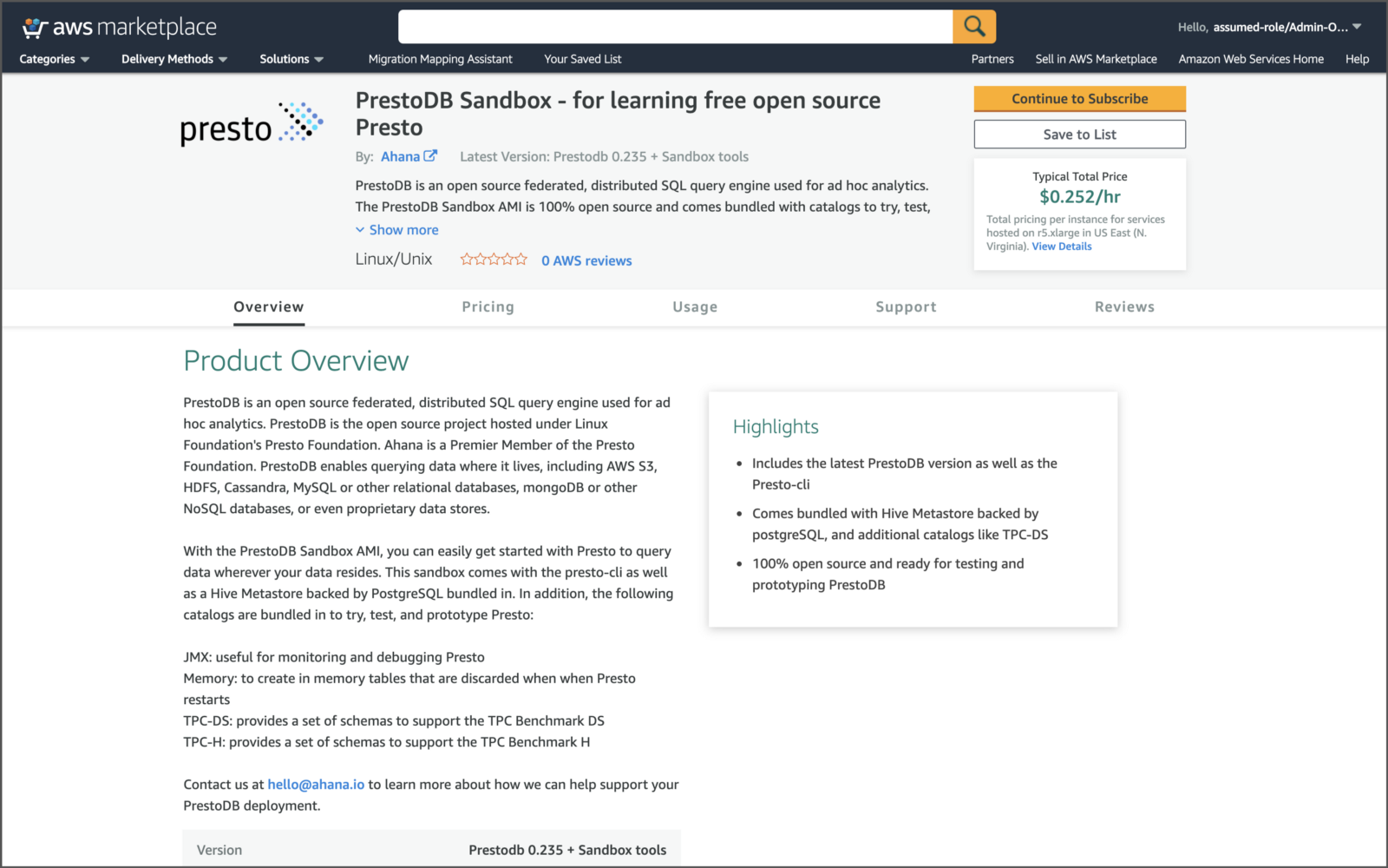
Ahana’s PrestoDB Sandbox AMI allows you to easily get started with Presto to query data wherever your data resides. This AMI configures a single EC2 instance Sandbox to be both the Presto Coordinator and a Presto Worker. It comes with an Apache Hive Metastore backed by PostgreSQL bundled in. In addition, the following catalogs are bundled in to try, test, and prototype with Presto:
- JMX: useful for monitoring and debugging Presto
- Memory: stores data and metadata in RAM, which is discarded when Presto restarts
- TPC-DS: provides a set of schemas to support the TPC Benchmark DS
- TPC-H: provides a set of schemas to support the TPC Benchmark H
Apache Hive
In this demonstration, we will use Apache Hive and an Apache Hive Metastore backed by PostgreSQL. Apache Hive is data warehouse software that facilitates reading, writing, and managing large datasets residing in distributed storage using SQL. The structure can be projected onto data already in storage. A command-line tool and JDBC driver are provided to connect users to Hive. The Metastore provides two essential features of a data warehouse: data abstraction and data discovery. Hive accomplishes both features by providing a metadata repository that is tightly integrated with the Hive query processing system so that data and metadata are in sync.
Getting Started
To get started creating federated queries with Presto, we first need to create and configure our AWS environment, as shown below.

Subscribe to Ahana’s PrestoDB Sandbox
To start, subscribe to Ahana’s PrestoDB Sandbox on AWS Marketplace. Make sure you are aware of the costs involved. The AWS current pricing for the default, Linux-based r5.xlarge on-demand EC2 instance hosted in US East (N. Virginia) is USD 0.252 per hour. For the demonstration, since performance is not an issue, you could try a smaller EC2 instance, such as r5.large instance costs USD 0.126 per hour.
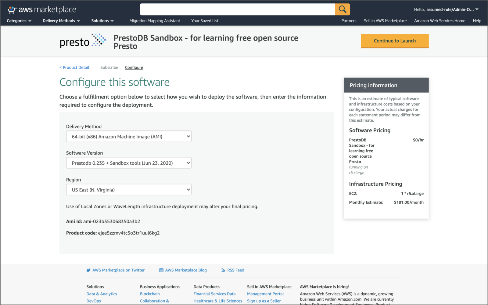
The configuration process will lead you through the creation of an EC2 instance based on Ahana’s PrestoDB Sandbox AMI.

I chose to create the EC2 instance in my default VPC. Part of the demonstration includes connecting to Presto locally using JDBC. Therefore, it was also necessary to include a public IP address for the EC2 instance. If you chose to do so, I strongly recommend limiting the required ports 22 and 8080 in the instance’s Security Group to just your IP address (a /32 CIDR block).

Lastly, we need to assign an IAM Role to the EC2 instance, which has access to Amazon S3. I assigned the AWS managed policy, AmazonS3FullAccess, to the EC2’s IAM Role.

AWS managed policy to the RolePart of the configuration also asks for a key pair. You can use an existing key or create a new key for the demo. For reference in future commands, I am using a key named ahana-presto and my key path of ~/.ssh/ahana-presto.pem. Be sure to update the commands to match your own key’s name and location.

Once complete, instructions for using the PrestoDB Sandbox EC2 are provided.
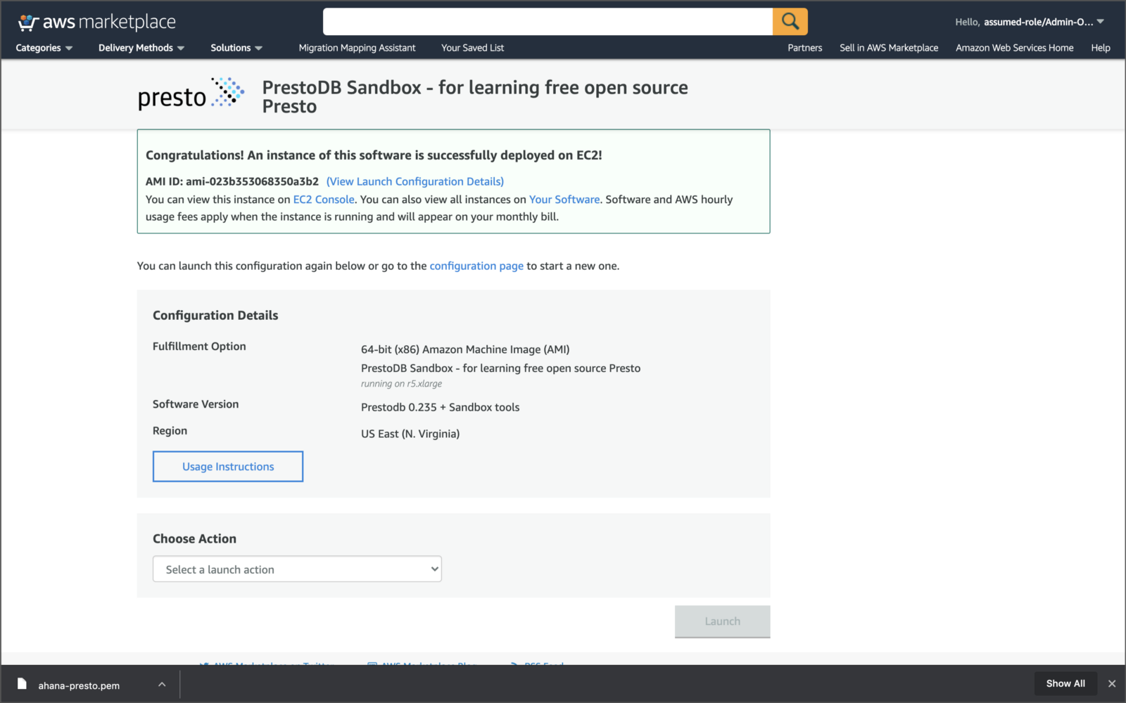


You can view the running EC2 instance, containing Presto, from the web-based AWS EC2 Management Console. Make sure to note the public IPv4 address or the public IPv4 DNS address as this value will be required during the demo.

AWS CloudFormation
We will use Amazon RDS for PostgreSQL and Amazon S3 as additional data sources for Presto. Included in the project files on GitHub is an AWS CloudFormation template, cloudformation/presto_ahana_demo.yaml. The template creates a single RDS for PostgreSQL instance in the default VPC and an encrypted Amazon S3 bucket.
All the source code for this post is on GitHub. Use the following command to git clone a local copy of the project.
git clone \
  –branch master –single-branch –depth 1 –no-tags \
  https://github.com/garystafford/presto-aws-federated-queries.git
To create the AWS CloudFormation stack from the template, cloudformation/rds_s3.yaml, execute the following aws cloudformation command. Make sure you change the DBAvailabilityZone parameter value (shown in bold) to match the AWS Availability Zone in which your Ahana PrestoDB Sandbox EC2 instance was created. In my case, us-east-1f.
aws cloudformation create-stack \
  --stack-name ahana-prestodb-demo \
  --template-body file://cloudformation/presto_ahana_demo.yaml \
  --parameters ParameterKey=DBAvailabilityZone,ParameterValue=us-east-1f
To ensure the RDS for PostgreSQL database instance can be accessed by Presto running on the Ahana PrestoDB Sandbox EC2, manually add the PrestoDB Sandbox EC2’s Security Group to port 5432 within the database instance’s VPC Security Group’s Inbound rules. I have also added my own IP to port 5432, which enables me to connect to the RDS instance directly from my IDE using JDBC.

The AWS CloudFormation stack’s Outputs tab includes a set of values, including the JDBC connection string for the new RDS for PostgreSQL instance, JdbcConnString, and the Amazon S3 bucket’s name, Bucket. All these values will be required during the demonstration.

Preparing the PrestoDB Sandbox
There are a few steps we need to take to properly prepare the PrestoDB Sandbox EC2 for our demonstration. First, use your PrestoDB Sandbox EC2 SSH key to scp the properties and sql directories to the Presto EC2 instance. First, you will need to set the EC2_ENDPOINT value (shown in bold) to your EC2’s public IPv4 address or public IPv4 DNS value. You can hardcode the value or use the aws ec2 API command is shown below to retrieve the value programmatically.
# on local workstation
EC2_ENDPOINT=$(aws ec2 describe-instances \
  --filters "Name=product-code,Values=ejee5zzmv4tc5o3tr1uul6kg2" \
    "Name=product-code.type,Values=marketplace" \
  --query "Reservations[*].Instances[*].{Instance:PublicDnsName}" \
  --output text)
scp -i "~/.ssh/ahana-presto.pem" \
  -r properties/ sql/ \
  ec2-user@${EC2_ENDPOINT}:~/
ssh -i "~/.ssh/ahana-presto.pem" ec2-user@${EC2_ENDPOINT}
Environment Variables
Next, we need to set several environment variables. First, replace the DATA_BUCKET and POSTGRES_HOST values below (shown in bold) to match your environment. The PGPASSWORD value should be correct unless you changed it in the CloudFormation template. Then, execute the command to add the variables to your .bash_profile file.
echo """
export DATA_BUCKET=prestodb-demo-databucket-CHANGE_ME
export POSTGRES_HOST=presto-demo.CHANGE_ME.us-east-1.rds.amazonaws.com
export PGPASSWORD=5up3r53cr3tPa55w0rd
export JAVA_HOME=/usr
export HADOOP_HOME=/home/ec2-user/hadoop
export HADOOP_CLASSPATH=$HADOOP_HOME/share/hadoop/tools/lib/*
export HIVE_HOME=/home/ec2-user/hive
export PATH=$HIVE_HOME/bin:$HADOOP_HOME/bin:$PATH
""" >>~/.bash_profile
Optionally, I suggest updating the EC2 instance with available updates and install your favorite tools, likehtop, to monitor the EC2 performance.
yes | sudo yum update
yes | sudo yum install htop

Before further configuration for the demonstration, let’s review a few aspects of the Ahana PrestoDB EC2 instance. There are several applications pre-installed on the instance, including Java, Presto, Hadoop, PostgreSQL, and Hive. Versions shown are current as of early September 2020.
java -version
  # openjdk version "1.8.0_252"
  # OpenJDK Runtime Environment (build 1.8.0_252-b09)
  # OpenJDK 64-Bit Server VM (build 25.252-b09, mixed mode)
hadoop version
  # Hadoop 2.9.2
postgres --version
  # postgres (PostgreSQL) 9.2.24
psql --version
  # psql (PostgreSQL) 9.2.24
hive --version
  # Hive 2.3.7
presto-cli --version
  # Presto CLI 0.235-cb21100
The Presto configuration files are in the /etc/presto/ directory. The Hive configuration files are in the ~/hive/conf/ directory. Here are a few commands you can use to gain a better understanding of their configurations.
ls /etc/presto/
cat /etc/presto/jvm.config
cat /etc/presto/config.properties
cat /etc/presto/node.properties
# installed and configured catalogs
ls /etc/presto/catalog/
cat ~/hive/conf/hive-site.xml
Configure Presto
To configure Presto, we need to create and copy a new Presto postgresql catalog properties file for the newly created RDS for PostgreSQL instance. Modify the properties/rds_postgresql.properties file, replacing the value, connection-url (shown in bold), with your own JDBC connection string, shown in the CloudFormation Outputs tab.
connector.name=postgresql
connection-url=jdbc:postgresql://presto-demo.abcdefg12345.us-east-1.rds.amazonaws.com:5432/shipping
connection-user=presto
connection-password=5up3r53cr3tPa55w0rd
Move the rds_postgresql.properties file to its correct location using sudo.
sudo mv properties/rds_postgresql.properties /etc/presto/catalog/
We also need to modify the existing Hive catalog properties file, which will allow us to write to non-managed Hive tables from Presto.
connector.name=hive-hadoop2
hive.metastore.uri=thrift://localhost:9083
hive.non-managed-table-writes-enabled=true
The following command will overwrite the existing hive.properties file with the modified version containing the new property.
sudo mv properties/hive.properties |
  /etc/presto/catalog/hive.properties
To finalize the configuration of the catalog properties files, we need to restart Presto. The easiest way is to reboot the EC2 instance, then SSH back into the instance. Since our environment variables are in the .bash_profile file, they will survive a restart and logging back into the EC2 instance.
sudo reboot
Add Tables to Apache Hive Metastore
We will use RDS for PostgreSQL and Apache Hive Metastore/Amazon S3 as additional data sources for our federated queries. The Ahana PrestoDB Sandbox instance comes pre-configured with Apache Hive and an Apache Hive Metastore, backed by PostgreSQL (a separate PostgreSQL 9.x instance pre-installed on the EC2).
The Sandbox’s instance of Presto comes pre-configured with schemas for the TPC Benchmark DS (TPC-DS). We will create identical tables in our Apache Hive Metastore, which correspond to three external tables in the TPC-DS data source’s sf1 schema: tpcds.sf1.customer, tpcds.sf1.customer_address, and tpcds.sf1.customer_demographics. A Hive external table describes the metadata/schema on external files. External table files can be accessed and managed by processes outside of Hive. As an example, here is the SQL statement that creates the external customer table in the Hive Metastore and whose data will be stored in the S3 bucket.
CREATE EXTERNAL TABLE IF NOT EXISTS `customer`(
  `c_customer_sk` bigint,
  `c_customer_id` char(16),
  `c_current_cdemo_sk` bigint,
  `c_current_hdemo_sk` bigint,
  `c_current_addr_sk` bigint,
  `c_first_shipto_date_sk` bigint,
  `c_first_sales_date_sk` bigint,
  `c_salutation` char(10),
  `c_first_name` char(20),
  `c_last_name` char(30),
  `c_preferred_cust_flag` char(1),
  `c_birth_day` integer,
  `c_birth_month` integer,
  `c_birth_year` integer,
  `c_birth_country` char(20),
  `c_login` char(13),
  `c_email_address` char(50),
  `c_last_review_date_sk` bigint)
STORED AS PARQUET
LOCATION
  's3a://prestodb-demo-databucket-CHANGE_ME/customer'
TBLPROPERTIES ('parquet.compression'='SNAPPY');
The threeCREATE EXTERNAL TABLE SQL statements are included in the sql/ directory: sql/hive_customer.sql, sql/hive_customer_address.sql, and sql/hive_customer_demographics.sql. The bucket name (shown in bold above), needs to be manually updated to your own bucket name in all three files before continuing.
Next, run the following hive commands to create the external tables in the Hive Metastore within the existing default schema/database.
hive --database default -f sql/hive_customer.sql
hive --database default -f sql/hive_customer_address.sql
hive --database default -f sql/hive_customer_demographics.sql
To confirm the tables were created successfully, we could use a variety of hive commands.
hive --database default -e "SHOW TABLES;"
hive --database default -e "DESCRIBE FORMATTED customer;"
hive --database default -e "SELECT * FROM customer LIMIT 5;"

Alternatively, you can also create the external table interactively from within Hive, using the hive command to access the CLI. Copy and paste the contents of the SQL files to the hive CLI. To exit hive use quit;.

Amazon S3 Data Source Setup
With the external tables created, we will now select all the data from each of the three tables in the TPC-DS data source and insert that data into the equivalent Hive tables. The physical data will be written to Amazon S3 as highly-efficient, columnar storage format, SNAPPY-compressed Apache Parquet files. Execute the following commands. I will explain why the customer_address table statements are a bit different, next.
# inserts 100,000 rows
presto-cli --execute """
  INSERT INTO hive.default.customer
  SELECT * FROM tpcds.sf1.customer;
  """
# inserts 50,000 rows across 52 partitions
presto-cli --execute """
  INSERT INTO hive.default.customer_address
  SELECT ca_address_sk, ca_address_id, ca_street_number,
    ca_street_name, ca_street_type, ca_suite_number,
    ca_city, ca_county, ca_zip, ca_country, ca_gmt_offset,
    ca_location_type, ca_state
  FROM tpcds.sf1.customer_address
  ORDER BY ca_address_sk;
  """
# add new partitions in metastore
hive -e "MSCK REPAIR TABLE default.customer_address;"
# inserts 1,920,800 rows
presto-cli --execute """
  INSERT INTO hive.default.customer_demographics
  SELECT * FROM tpcds.sf1.customer_demographics;
  """
Confirm the data has been loaded into the correct S3 bucket locations and is in Parquet-format using the AWS Management Console or AWS CLI. Rest assured, the Parquet-format data is SNAPPY-compressed even though the S3 console incorrectly displays Compression as None. You can easily confirm the compression codec with a utility like parquet-tools.


Partitioned Tables
The customer_address table is unique in that it has been partitioned by the ca_state column. Partitioned tables are created using the PARTITIONED BY clause.
CREATE EXTERNAL TABLE `customer_address`(
    `ca_address_sk` bigint,
    `ca_address_id` char(16),
    `ca_street_number` char(10),
    `ca_street_name` char(60),
    `ca_street_type` char(15),
    `ca_suite_number` char(10),
    `ca_city` varchar(60),
    `ca_county` varchar(30),
    `ca_zip` char(10),
    `ca_country` char(20),
    `ca_gmt_offset` double precision,
    `ca_location_type` char(20)
)
PARTITIONED BY (`ca_state` char(2))
STORED AS PARQUET
LOCATION
  's3a://prestodb-demo-databucket-CHANGE_ME/customer'
TBLPROPERTIES ('parquet.compression'='SNAPPY');
According to Apache Hive, a table can have one or more partition columns and a separate data directory is created for each distinct value combination in the partition columns. Since the data for the Hive tables are stored in Amazon S3, that means that when the data is written to the customer_address table, it is automatically separated into different S3 key prefixes based on the state. The data is physically “partitioned”.

Whenever add new partitions in S3, we need to run the MSCK REPAIR TABLE command to add that table’s new partitions to the Hive Metastore.
hive -e "MSCK REPAIR TABLE default.customer_address;"
In SQL, a predicate is a condition expression that evaluates to a Boolean value, either true or false. Defining the partitions aligned with the attributes that are frequently used in the conditions/filters (predicates) of the queries can significantly increase query efficiency. When we execute a query that uses an equality comparison condition, such as ca_state = 'TN', partitioning means the query will only work with a slice of the data in the corresponding ca_state=TN prefix key. There are 50,000 rows of data in the customer_address table, but only 1,418 rows (2.8% of the total data) in the ca_state=TN partition. With the additional advantage of Parquet format with SNAPPY compression, partitioning can significantly reduce query execution time.
Adding Data to RDS for PostgreSQL Instance
For the demonstration, we will also replicate the schema and data of the tpcds.sf1.customer_address table to the new RDS for PostgreSQL instance’s shipping database.
CREATE TABLE customer_address (
    ca_address_sk bigint,
    ca_address_id char(16),
    ca_street_number char(10),
    ca_street_name char(60),
    ca_street_type char(15),
    ca_suite_number char(10),
    ca_city varchar(60),
    ca_county varchar(30),
    ca_state char(2),
    ca_zip char(10),
    ca_country char(20),
    ca_gmt_offset double precision,
    ca_location_type char(20)
);
Like Hive and Presto, we can create the table programmatically from the command line or interactively; I prefer the programmatic approach. Use the following psql command, we can create the customer_address table in the public schema of the shipping database.
psql -h ${POSTGRES_HOST} -p 5432 -d shipping -U presto \
  -f sql/postgres_customer_address.sql
Now, to insert the data into the new PostgreSQL table, run the following presto-cli command.
# inserts 50,000 rows
presto-cli --execute """
  INSERT INTO rds_postgresql.public.customer_address
  SELECT * FROM tpcds.sf1.customer_address;
  """
To confirm that the data was imported properly, we can use a variety of commands.
-- Should be 50000 rows in table
psql -h ${POSTGRES_HOST} -p 5432 -d shipping -U presto \
  -c "SELECT COUNT(*) FROM customer_address;"
psql -h ${POSTGRES_HOST} -p 5432 -d shipping -U presto \
  -c "SELECT * FROM customer_address LIMIT 5;"
Alternatively, you could use the PostgreSQL client interactively by copying and pasting the contents of the sql/postgres_customer_address.sql file to the psql command prompt. To interact with PostgreSQL from the psql command prompt, use the following command.
psql -h ${POSTGRES_HOST} -p 5432 -d shipping -U presto
Use the \dt command to list the PostgreSQL tables and the \q command to exit the PostgreSQL client. We now have all the new data sources created and configured for Presto!
Interacting with Presto
Presto provides a web interface for monitoring and managing queries. The interface provides dashboard-like insights into the Presto Cluster and queries running on the cluster. The Presto UI is available on port 8080 using the public IPv4 address or the public IPv4 DNS.

There are several ways to interact with Presto, via the PrestoDB Sandbox. The post will demonstrate how to execute ad-hoc queries against Presto from an IDE using a JDBC connection and the Presto CLI. Other options include running queries against Presto from Java and Python applications, Tableau, or Apache Spark/PySpark.
Below, we see a query being run against Presto from JetBrains PyCharm, using a Java Database Connectivity (JDBC) connection. The advantage of using an IDE like JetBrains is having a single visual interface, including all the project files, multiple JDBC configurations, output results, and the ability to run multiple ad hoc queries.

Below, we see an example of configuring the Presto Data Source using the JDBC connection string, supplied in the CloudFormation stack Outputs tab.

Make sure to download and use the latest Presto JDBC driver JAR.

With JetBrains’ IDEs, we can even limit the databases/schemas displayed by the Data Source. This is helpful when we have multiple Presto catalogs configured, but we are only interested in certain data sources.

We can also run queries using the Presto CLI, three different ways. We can pass a SQL statement to the Presto CLI, pass a file containing a SQL statement to the Presto CLI, or work interactively from the Presto CLI. Below, we see a query being run, interactively from the Presto CLI.
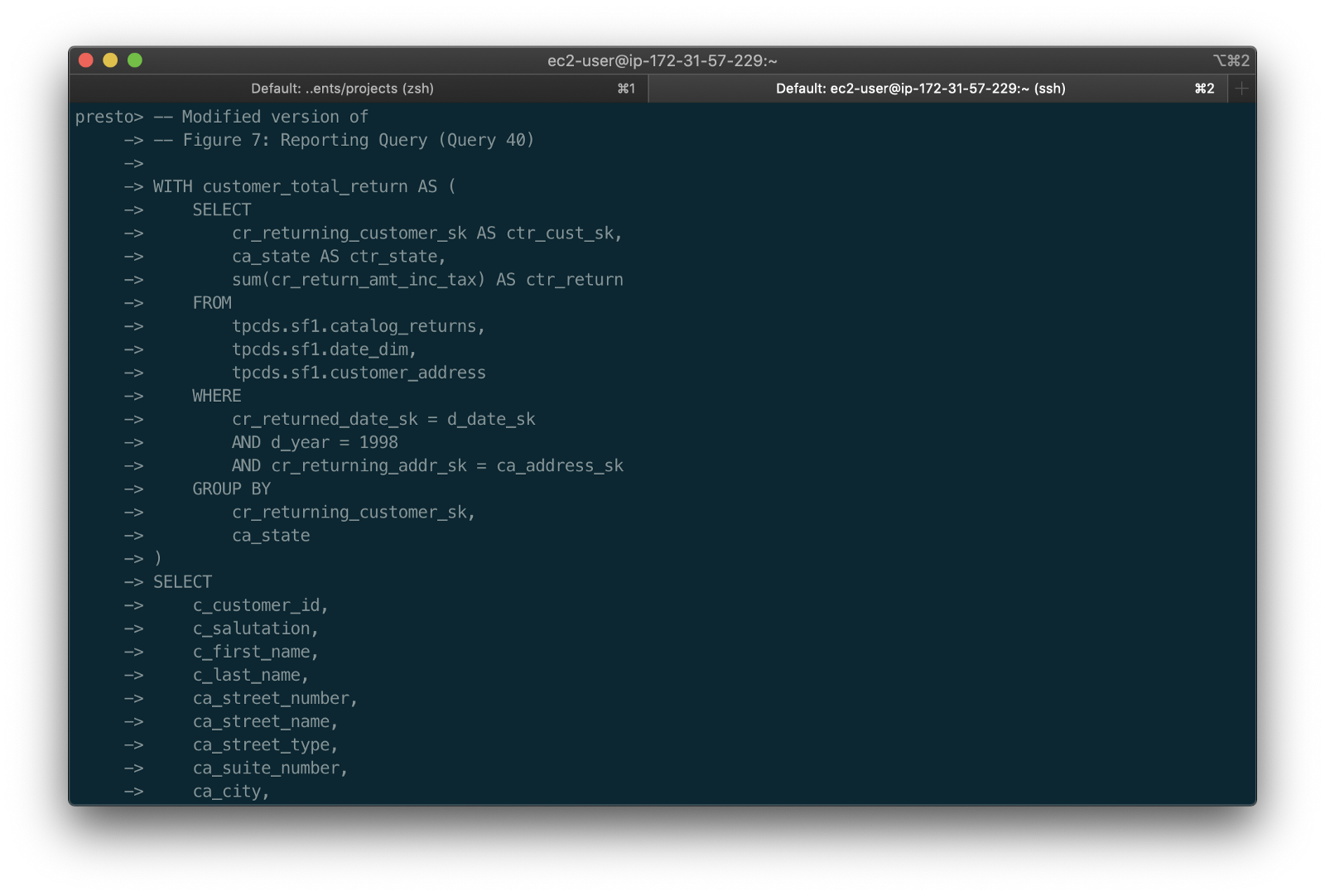
As the query is running, we can observe the live Presto query statistics (not very user friendly in my terminal).

And finally, the view the query results.

Federated Queries
The example queries used in the demonstration and included in the project were mainly extracted from the scholarly article, Why You Should Run TPC-DS: A Workload Analysis, available as a PDF on the tpc.org website. I have modified the SQL queries to work with Presto.
In the first example, we will run the three versions of the same basic query statement. Version 1 of the query is not a federated query; it only queries a single data source. Version 2 of the query queries two different data sources. Finally, version 3 of the query queries three different data sources. Each of the three versions of the SQL statement should return the same results — 93 rows of data.
Version 1: Single Data Source
The first version of the query statement, sql/presto_query2.sql, is not a federated query. Each of the query’s four tables (catalog_returns, date_dim, customer, and customer_address) reference the TPC-DS data source, which came pre-installed with the PrestoDB Sandbox. Note table references on lines 11–13 and 41–42 are all associated with the tpcds.sf1 schema.
We will run each query non-interactively using the presto-cli. We will choose the sf1 (scale factor of 1) tpcds schema. According to Presto, every unit in the scale factor (sf1, sf10, sf100) corresponds to a gigabyte of data.
presto-cli \
  --catalog tpcds \
  --schema sf1 \
  --file sql/presto_query2.sql \
  --output-format ALIGNED \
  --client-tags "presto_query2"
Below, we see the query results in the presto-cli.

Below, we see the first query running in Presto’s web interface.

Below, we see the first query’s results detailed in Presto’s web interface.

Version 2: Two Data Sources
In the second version of the query statement, sql/presto_query2_federated_v1.sql, two of the tables (catalog_returns and date_dim) reference the TPC-DS data source. The other two tables (customer and customer_address) now reference the Apache Hive Metastore for their schema and underlying data in Amazon S3. Note table references on lines 11 and 12, as opposed to lines 13, 41, and 42.
Again, run the query using the presto-cli.
presto-cli \
  --catalog tpcds \
  --schema sf1 \
  --file sql/presto_query2_federated_v1.sql \
  --output-format ALIGNED \
  --client-tags "presto_query2_federated_v1"
Below, we see the second query’s results detailed in Presto’s web interface.

Even though the data is in two separate and physically different data sources, we can easily query it as though it were all in the same place.
Version 3: Three Data Sources
In the third version of the query statement, sql/presto_query2_federated_v2.sql, two of the tables (catalog_returns and date_dim) reference the TPC-DS data source. One of the tables (hive.default.customer) references the Apache Hive Metastore. The fourth table (rds_postgresql.public.customer_address) references the new RDS for PostgreSQL database instance. The underlying data is in Amazon S3. Note table references on lines 11 and 12, and on lines 13 and 41, as opposed to line 42.
Again, we have run the query using the presto-cli.
presto-cli \
  --catalog tpcds \
  --schema sf1 \
  --file sql/presto_query2_federated_v2.sql \
  --output-format ALIGNED \
  --client-tags "presto_query2_federated_v2"
Below, we see the third query’s results detailed in Presto’s web interface.

Again, even though the data is in three separate and physically different data sources, we can easily query it as though it were all in the same place.
Additional Query Examples
The project contains several additional query statements, which I have extracted from Why You Should Run TPC-DS: A Workload Analysis and modified work with Presto and federate across multiple data sources.
# non-federated
presto-cli \
  --catalog tpcds \
  --schema sf1 \
  --file sql/presto_query1.sql \
  --output-format ALIGNED \
  --client-tags "presto_query1"
# federated - two sources
presto-cli \
  --catalog tpcds \
  --schema sf1 \
  --file sql/presto_query1_federated.sql \
  --output-format ALIGNED \
  --client-tags "presto_query1_federated"
# non-federated
presto-cli \
  --catalog tpcds \
  --schema sf1 \
  --file sql/presto_query4.sql \
  --output-format ALIGNED \
  --client-tags "presto_query4"
# federated - three sources
presto-cli \
  --catalog tpcds \
  --schema sf1 \
  --file sql/presto_query4_federated.sql \
  --output-format ALIGNED \
  --client-tags "presto_query4_federated"
# non-federated
presto-cli \
  --catalog tpcds \
  --schema sf1 \
  --file sql/presto_query5.sql \
  --output-format ALIGNED \
  --client-tags "presto_query5"
Conclusion
In this post, we gained a better understanding of Presto using Ahana’s PrestoDB Sandbox product from AWS Marketplace. We learned how Presto queries data where it lives, including Apache Hive, Thrift, Kafka, Kudu, and Cassandra, Elasticsearch, MongoDB, etc. We also learned about Apache Hive and the Apache Hive Metastore, Apache Parquet file format, and how and why to partition Hive data in Amazon S3. Most importantly, we learned how to write federated queries that join multiple disparate data sources without having to move the data into a single monolithic data store.
This blog represents my own viewpoints and not of my employer, Amazon Web Services.
Getting Started with IoT Analytics on AWS
Posted by Gary A. Stafford in AWS, Bash Scripting, Big Data, Cloud, Python, Software Development, Technology Consulting on July 15, 2020
Introduction
AWS defines AWS IoT as a set of managed services that enable ‘internet-connected devices to connect to the AWS Cloud and lets applications in the cloud interact with internet-connected devices.’ AWS IoT services span three categories: Device Software, Connectivity and Control, and Analytics. In this post, we will focus on AWS IoT Analytics, one of four services, which are part of the AWS IoT Analytics category. According to AWS, AWS IoT Analytics is a fully-managed IoT analytics service, designed specifically for IoT, which collects, pre-processes, enriches, stores, and analyzes IoT device data at scale.
Certainly, AWS IoT Analytics is not the only way to analyze the Internet of Things (IoT) or Industrial Internet of Things (IIoT) data on AWS. It is common to see Data Analyst teams using a more general AWS data analytics stack, composed of Amazon S3, Amazon Kinesis, AWS Glue, and Amazon Athena or Amazon Redshift and Redshift Spectrum, for analyzing IoT data. So then why choose AWS IoT Analytics over a more traditional AWS data analytics stack? According to AWS, IoT Analytics was purpose-built to manage the complexities of IoT and IIoT data on a petabyte-scale. According to AWS, IoT data frequently has significant gaps, corrupted messages, and false readings that must be cleaned up before analysis can occur. Additionally, IoT data must often be enriched and transformed to be meaningful. IoT Analytics can filter, transform, and enrich IoT data before storing it in a time-series data store for analysis.
In the following post, we will explore the use of AWS IoT Analytics to analyze environmental sensor data, in near real-time, from a series of IoT devices. To follow along with the post’s demonstration, there is an option to use sample data to simulate the IoT devices (see the ‘Simulating IoT Device Messages’ section of this post).
IoT Devices
In this post, we will explore IoT Analytics using IoT data generated from a series of custom-built environmental sensor arrays. Each breadboard-based sensor array is connected to a Raspberry Pi single-board computer (SBC), the popular, low cost, credit-card sized Linux computer. The IoT devices were purposely placed in physical locations that vary in temperature, humidity, and other environmental conditions.

Each device includes the following sensors:
- MQ135 Air Quality Sensor Hazardous Gas Detection Sensor: CO, LPG, Smoke (link)
(requires an MCP3008 – 8-Channel 10-Bit ADC w/ SPI Interface (link)) - DHT22/AM2302 Digital Temperature and Humidity Sensor (link)
- Onyehn IR Pyroelectric Infrared PIR Motion Sensor (link)
- Anmbest Light Intensity Detection Photosensitive Sensor (link)

AWS IoT Device SDK
Each Raspberry Pi device runs a custom Python script, sensor_collector_v2.py. The script uses the AWS IoT Device SDK for Python v2 to communicate with AWS. The script collects a total of seven different readings from the four sensors at a regular interval. Sensor readings include temperature, humidity, carbon monoxide (CO), liquid petroleum gas (LPG), smoke, light, and motion.
The script securely publishes the sensor readings, along with a device ID and timestamp, as a single message, to AWS using the ISO standard Message Queuing Telemetry Transport (MQTT) network protocol. Below is an example of an MQTT message payload, published by the collector script.
This file contains bidirectional Unicode text that may be interpreted or compiled differently than what appears below. To review, open the file in an editor that reveals hidden Unicode characters.
Learn more about bidirectional Unicode characters
| { | |
| "data": { | |
| "co": 0.006104480269226063, | |
| "humidity": 55.099998474121094, | |
| "light": true, | |
| "lpg": 0.008895956948783413, | |
| "motion": false, | |
| "smoke": 0.023978358312270912, | |
| "temp": 31.799999237060547 | |
| }, | |
| "device_id": "6e:81:c9:d4:9e:58", | |
| "ts": 1594419195.292461 | |
| } |
As shown below, using tcpdump on the IoT device, the MQTT message payloads generated by the script average approximately 275 bytes. The complete MQTT messages average around 300 bytes.

AWS IoT Core
Each Raspberry Pi is registered with AWS IoT Core. IoT Core allows users to quickly and securely connect devices to AWS. According to AWS, IoT Core can reliably scale to billions of devices and trillions of messages. Registered devices are referred to as things in AWS IoT Core. A thing is a representation of a specific device or logical entity. Information about a thing is stored in the registry as JSON data.
IoT Core provides a Device Gateway, which manages all active device connections. The Gateway currently supports MQTT, WebSockets, and HTTP 1.1 protocols. Behind the Message Gateway is a high-throughput pub/sub Message Broker, which securely transmits messages to and from all IoT devices and applications with low latency. Below, we see a typical AWS IoT Core architecture.
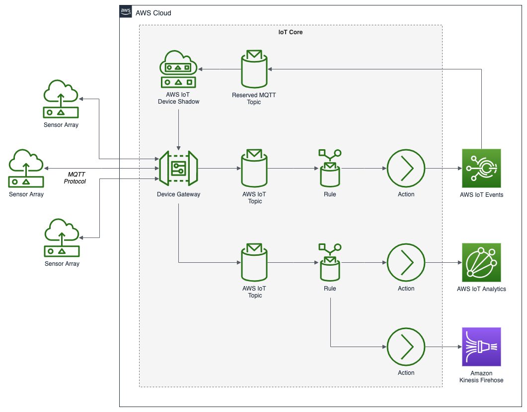
At a message frequency of five seconds, the three Raspberry Pi devices publish a total of roughly 50,000 IoT messages per day to AWS IoT Core.

AWS IoT Security
AWS IoT Core provides mutual authentication and encryption, ensuring all data is exchanged between AWS and the devices are secure by default. In the demo, all data is sent securely using Transport Layer Security (TLS) 1.2 with X.509 digital certificates on port 443. Authorization of the device to access any resource on AWS is controlled by individual AWS IoT Core Policies, similar to AWS IAM Policies. Below, we see an example of an X.509 certificate, assigned to a registered device.

AWS IoT Core Rules
Once an MQTT message is received from an IoT device (a thing), we use AWS IoT Rules to send message data to an AWS IoT Analytics Channel. Rules give your devices the ability to interact with AWS services. Rules are written in standard Structured Query Language (SQL). Rules are analyzed, and Actions are performed based on the MQTT topic stream. Below, we see an example rule that forwards our messages to IoT Analytics, in addition to AWS IoT Events and Amazon Kinesis Data Firehose.

Simulating IoT Device Messages
Building and configuring multiple Raspberry Pi-based sensor arrays, and registering the devices with AWS IoT Core would require a lot of work just for this post. Therefore, I have provided everything you need to simulate the three IoT devices, on GitHub. Use the following command to git clone a local copy of the project.
This file contains bidirectional Unicode text that may be interpreted or compiled differently than what appears below. To review, open the file in an editor that reveals hidden Unicode characters.
Learn more about bidirectional Unicode characters
| git clone \ | |
| –branch master –single-branch –depth 1 –no-tags \ | |
| https://github.com/garystafford/aws-iot-analytics-demo.git |
AWS CloudFormation
Use the CloudFormation template, iot-analytics.yaml, to create an IoT Analytics stack containing (17) resources, including the following.
- (3) AWS IoT Things
- (1) AWS IoT Core Topic Rule
- (1) AWS IoT Analytics Channel, Pipeline, Data store, and Data set
- (1) AWS Lambda and Lambda Permission
- (1) Amazon S3 Bucket
- (1) Amazon SageMaker Notebook Instance
- (5) AWS IAM Roles
Please be aware of the costs involved with the AWS resources used in the CloudFormation template before continuing. To build the AWS CloudFormation stack, run the following AWS CLI command.
This file contains bidirectional Unicode text that may be interpreted or compiled differently than what appears below. To review, open the file in an editor that reveals hidden Unicode characters.
Learn more about bidirectional Unicode characters
| aws cloudformation create-stack \ | |
| –stack-name iot-analytics-demo \ | |
| –template-body file://cloudformation/iot-analytics.yaml \ | |
| –parameters ParameterKey=ProjectName,ParameterValue=iot-analytics-demo \ | |
| ParameterKey=IoTTopicName,ParameterValue=iot-device-data \ | |
| –capabilities CAPABILITY_NAMED_IAM |
Below, we see a successful deployment of the IoT Analytics Demo CloudFormation Stack.

Publishing Sample Messages
Once the CloudFormation stack is created successfully, use an included Python script, send_sample_messages.py, to send sample IoT data to an AWS IoT Topic, from your local machine. The script will use your AWS identity and credentials, instead of an actual IoT device registered with IoT Core. The IoT data will be intercepted by an IoT Topic Rule and redirected, using a Topic Rule Action, to the IoT Analytics Channel.
First, we will ensure the IoT stack is running correctly on AWS by sending a few test messages. Go to the AWS IoT Core Test tab. Subscribe to the iot-device-data topic.

Then, run the following command using the smaller data file, raw_data_small.json.
This file contains bidirectional Unicode text that may be interpreted or compiled differently than what appears below. To review, open the file in an editor that reveals hidden Unicode characters.
Learn more about bidirectional Unicode characters
| cd sample_data/ | |
| time python3 ./send_sample_messages.py \ | |
| -f raw_data_small.json -t iot-device-data |
If successful, you should see the five messages appear in the Test tab, shown above. Example output from the script is shown below.

Then, run the second command using the larger data file, raw_data_large.json, containing 9,995 messages (a few hours worth of data). The command will take approximately 12 minutes to complete.
This file contains bidirectional Unicode text that may be interpreted or compiled differently than what appears below. To review, open the file in an editor that reveals hidden Unicode characters.
Learn more about bidirectional Unicode characters
| time python3 ./send_sample_messages.py \ | |
| -f raw_data_large.json -t iot-device-data |
Once the second command completes successfully, your IoT Analytics Channel should contain 10,000 unique messages. There is an optional extra-large data file containing approximately 50,000 IoT messages (24 hours of IoT messages).
AWS IoT Analytics
AWS IoT Analytics is composed of five primary components: Channels, Pipelines, Data stores, Data sets, and Notebooks. These components enable you to collect, prepare, store, analyze, and visualize your IoT data.

Below, we see a typical AWS IoT Analytics architecture. IoT messages are pulled from AWS IoT Core, thought a Rule Action. Amazon QuickSight provides business intelligence, visualization. Amazon QuickSight ML Insights adds anomaly detection and forecasting.

IoT Analytics Channel
An AWS IoT Analytics Channel pulls messages or data into IoT Analytics from other AWS sources, such as Amazon S3, Amazon Kinesis, or Amazon IoT Core. Channels store data for IoT Analytics Pipelines. Both Channels and Data store support storing data in your own Amazon S3 bucket or in an IoT Analytics service-managed S3 bucket. In the demonstration, we are using a service managed S3 bucket.
When creating a Channel, you also decide how long to retain the data. For the demonstration, we have set the data retention period for 14 days. Channels are generally not used for long term storage of data. Typically, you would only retain data in the Channel for the time period you need to analyze. For long term storage of IoT message data, I recommend using an AWS IoT Core Rule to send a copy of the raw IoT data to Amazon S3, using a service such as Amazon Kinesis Data Firehose.

IoT Analytics Pipeline
An AWS IoT Analytics Pipeline consumes messages from one or more Channels. Pipelines transform, filter, and enrich the messages before storing them in IoT Analytics Data stores. A Pipeline is composed of an array of activities. Logically, you must specify both a Channel (source) and a Datastore (destination) activity. Optionally, you may choose as many as 23 additional activities in the pipelineActivities array.
In our demonstration’s Pipeline, iot_analytics_pipeline, we have specified five additional activities, including DeviceRegistryEnrich, Filter, Math, Lambda, and SelectAttributes. There are two additional Activity types we did not choose, RemoveAttributes and AddAttributes.

The demonstration’s Pipeline created by CloudFormation starts with messages from the demonstration’s Channel, iot_analytics_channel, similar to the following.
This file contains bidirectional Unicode text that may be interpreted or compiled differently than what appears below. To review, open the file in an editor that reveals hidden Unicode characters.
Learn more about bidirectional Unicode characters
| { | |
| "co": 0.004782974313835918, | |
| "device_id": "ae:c4:1d:34:1c:7b", | |
| "device": "iot-device-01", | |
| "humidity": 68.81000305175781, | |
| "light": true, | |
| "lpg": 0.007456714657976871, | |
| "msg_received": "2020-07-13T19:44:58.690+0000", | |
| "motion": false, | |
| "smoke": 0.019858593777432054, | |
| "temp": 19.200000762939453, | |
| "ts": 1594496359.235107 | |
| } |
The demonstration’s Pipeline transforms the messages through a series of Pipeline Activities and then stores the resulting message in the demonstration’s Data store, iot_analytics_data_store. The resulting messages appear similar to the following.
This file contains bidirectional Unicode text that may be interpreted or compiled differently than what appears below. To review, open the file in an editor that reveals hidden Unicode characters.
Learn more about bidirectional Unicode characters
| { | |
| "co": 0.0048, | |
| "device": "iot-device-01", | |
| "humidity": 68.81, | |
| "light": true, | |
| "lpg": 0.0075, | |
| "metadata": "{defaultclientid=iot-device-01, thingname=iot-device-01, thingid=5de1c2af-14b4-49b5-b20b-b25cf251b01a, thingarn=arn:aws:iot:us-east-1:864887685992:thing/iot-device-01, thingtypename=null, attributes={installed=1594665292, latitude=37.4133144, longitude=-122.1513069}, version=2, billinggroupname=null}", | |
| "msg_received": "2020-07-13T19:44:58.690+0000", | |
| "motion": false, | |
| "smoke": 0.0199, | |
| "temp": 66.56, | |
| "ts": 1594496359.235107 | |
| } |
In our demonstration, transformations to the messages include dropping the device_id attribute and converting the temp attribute value to Fahrenheit. In addition, the Lambda Activity rounds down the temp, humidity, co, lpg, and smoke attribute values to between 2–4 decimal places of precision.

The demonstration’s Pipeline also enriches the message with the metadata attribute, containing metadata from the IoT device’s AWS IoT Core Registry. The metadata includes additional information about the device that generated the message, including custom attributes we input, such as location (longitude and latitude) and the device’s installation date.

A significant feature of Pipelines is the ability to reprocess messages. If you make a change to the Pipeline, which often happens during the data preparation stage, you can reprocess any or all messages in the associated Channel, and overwrite the messages in the Data set.

IoT Analytics Data store
An AWS IoT Analytics Data store stores prepared data from an AWS IoT Analytics Pipeline, in a fully-managed database. Both Channels and Data store support storing data in your own Amazon S3 bucket or in an IoT Analytics managed S3 bucket. In the demonstration, we are using a service-managed S3 bucket to store messages in our Data store.

IoT Analytics Data set
An AWS IoT Analytics Data set automatically provides regular, up-to-date insights for data analysts by querying a Data store using standard SQL. Regular updates are provided through the use of a cron expression. For the demonstration, we are using a 15-minute interval.
Below, we see the sample messages in the Result preview pane of the Data set. These are the five test messages we sent to check the stack. Note the SQL query used to obtain the messages, which queries the Data store. The Data store, as you will recall, contains the transformed messages from the Pipeline.

IoT Analytics Data sets also support sending content results, which are materialized views of your IoT Analytics data, to an Amazon S3 bucket.

The CloudFormation stack contains an encrypted Amazon S3 Bucket. This bucket receives a copy of the messages from the IoT Analytics Data set whenever the scheduled update is run by the cron expression.

IoT Analytics Notebook
An AWS IoT Analytics Notebook allows users to perform statistical analysis and machine learning on IoT Analytics Data sets using Jupyter Notebooks. The IoT Analytics Notebook service includes a set of notebook templates that contain AWS-authored machine learning models and visualizations. Notebooks Instances can be linked to a GitHub or other source code repository. Notebooks created with IoT Analytics Notebook can also be accessed directly through Amazon SageMaker. For the demonstration, the Notebooks Instance is associated with the project’s GitHub repository.

The repository contains a sample Jupyter Notebook, IoT_Analytics_Demo_Notebook.ipynb, based on the conda_python3 kernel. This preinstalled environment includes the default Anaconda installation and Python 3. The Notebook uses pandas, matplotlib, and plotly to manipulate and visualize the sample IoT messages we published earlier and stored in the Data set.


Notebooks can be modified, and the changes pushed back to GitHub. You could easily fork a copy of my GitHub repository and modify the CloudFormation template, to include your own GitHub repository URL.

Amazon QuickSight
Amazon QuickSight provides business intelligence (BI) and visualization. Amazon QuickSight ML Insights adds anomaly detection and forecasting. We can use Amazon QuickSight to visualize the IoT message data, stored in the IoT Analytics Data set.
Amazon QuickSight has both a Standard and an Enterprise Edition. AWS provides a detailed product comparison of each edition. For the post, I am demonstrating the Enterprise Edition, which includes additional features, such as ML Insights, hourly refreshes of SPICE (super-fast, parallel, in-memory, calculation engine), and theme customization. Please be aware of the costs of Amazon QuickSight if you choose to follow along with this part of the demo. Amazon QuickSight is enabled or configured with the demonstration’s CloudFormation template.
QuickSight Data Sets
Amazon QuickSight has a wide variety of data source options for creating Amazon QuickSight Data sets, including the ones shown below. Do not confuse Amazon QuickSight Data sets with IoT Analytics Data sets. These are two different, yet similar, constructs.

For the demonstration, we will create an Amazon QuickSight Data set that will use our IoT Analytics Data set as a data source.

Amazon QuickSight gives you the ability to modify QuickSight Data sets. For the demonstration, I have added two additional fields, converting the boolean light and motion values of true and false to binary values of 0 or 1. I have also deselected two fields that I do not need for QuickSight Analysis.

QuickSight provides a wide variety of functions, enabling us to perform dynamic calculations on the field values. Below, we see a new calculated field, light_dec, containing the original light field’s Boolean values converted to binary values. I am using a if...else formula to change the field’s value depending on the value in another field.

QuickSight Analysis
Using the QuickSight Data set, built from the IoT Analytics Data set as a data source, we create a QuickSight Analysis. The QuickSight Analysis user interface is shown below. An Analysis is primarily a collection of Visuals (Visual types). QuickSight provides a number of Visual types. Each visual is associated with a Data set. Data for the QuickSight Analysis or for each individual visual can be filtered. For the demo, I have created a QuickSight Analysis, including several typical QuickSight Visuals.

QuickSight Dashboards
To share a QuickSight Analysis, we can create a QuickSight Dashboard. Below, we see a few views of the QuickSight Analysis, shown above, as a Dashboard. A viewer of the Dashboard cannot edit the visuals, though they can apply filtering and interactively drill-down into data in the Visuals.


Geospatial Data
Amazon QuickSight understands geospatial data. If you recall, in the IoT Analytics Pipeline, we enriched the messages in the metadata from the device registry. The metadata attributes contained the device’s longitude and latitude. Quicksight will recognize those fields as geographic fields. In our QuickSight Analysis, we can visualize the geospatial data, using the geospatial chart (map) Visual type.

QuickSight Mobile App
Amazon QuickSight offers free iOS and Android versions of the Amazon QuickSight Mobile App. The mobile application makes it easy for registered QuickSight end-users to securely connect to QuickSight Dashboards, using their mobile devices. Below, we see two views of the same Dashboard, shown in the iOS version of the Amazon QuickSight Mobile App.

Amazon QuickSight ML Insights
According to Amazon, ML Insights leverages AWS’s machine learning (ML) and natural language capabilities to gain deeper insights from data. QuickSight’s ML-powered Anomaly Detection continuously analyze data to discover anomalies and variations inside of the aggregates, giving you the insights to act when business changes occur. QuickSight’s ML-powered Forecasting can be used to accurately predict your business metrics, and perform interactive what-if analysis with point-and-click simplicity. QuickSight’s built-in algorithms make it easy for anyone to use ML that learns from your data patterns to provide you with accurate predictions based on historical trends.
Below, we see the ML Insights tab in the demonstration’s QuickSight Analysis. Individually detected anomalies can be added to the QuickSight Analysis, similar to Visuals, and configured to tune the detection parameters.

Below, we see an example of humidity anomalies across all devices, based on their Anomaly Score and are higher or lower with a minimum delta of five percent.

Cleaning Up
You are charged hourly for the SageMaker Notebook Instance. Do not forget to delete your CloudFormation stack when you are done with the demonstration. Note the Amazon S3 bucket will not be deleted; you must do this manually.
This file contains bidirectional Unicode text that may be interpreted or compiled differently than what appears below. To review, open the file in an editor that reveals hidden Unicode characters.
Learn more about bidirectional Unicode characters
| aws cloudformation delete-stack \ | |
| –stack-name iot-analytics-demo |
Conclusion
In this post, we demonstrated how to use AWS IoT Analytics to analyze and visualize streaming messages from multiple IoT devices, in near real-time. Combined with other AWS IoT analytics services, such as AWS IoT SiteWise, AWS IoT Events, and AWS IoT Things Graph, you can create a robust, full-featured IoT Analytics platform, capable of handling millions of industrial, commercial, and residential IoT devices, generating petabytes of data.
This blog represents my own viewpoints and not of my employer, Amazon Web Services.
Getting Started with Data Analysis on AWS using AWS Glue, Amazon Athena, and QuickSight: Part 1
Posted by Gary A. Stafford in AWS, Bash Scripting, Big Data, Cloud, Python, Serverless, Software Development on January 5, 2020
Introduction
According to Wikipedia, data analysis is “a process of inspecting, cleansing, transforming, and modeling data with the goal of discovering useful information, informing conclusion, and supporting decision-making.” In this two-part post, we will explore how to get started with data analysis on AWS, using the serverless capabilities of Amazon Athena, AWS Glue, Amazon QuickSight, Amazon S3, and AWS Lambda. We will learn how to use these complementary services to transform, enrich, analyze, and visualize semi-structured data.
Data Analysis—discovering useful information, informing conclusion, and supporting decision-making. –Wikipedia
In part one, we will begin with raw, semi-structured data in multiple formats. We will discover how to ingest, transform, and enrich that data using Amazon S3, AWS Glue, Amazon Athena, and AWS Lambda. We will build an S3-based data lake, and learn how AWS leverages open-source technologies, such as Presto, Apache Hive, and Apache Parquet. In part two, we will learn how to further analyze and visualize the data using Amazon QuickSight. Here’s a quick preview of what we will build in part one of the post.
Demonstration
In this demonstration, we will adopt the persona of a large, US-based electric energy provider. The energy provider has developed its next-generation Smart Electrical Monitoring Hub (Smart Hub). They have sold the Smart Hub to a large number of residential customers throughout the United States. The hypothetical Smart Hub wirelessly collects detailed electrical usage data from individual, smart electrical receptacles and electrical circuit meters, spread throughout the residence. Electrical usage data is encrypted and securely transmitted from the customer’s Smart Hub to the electric provider, who is running their business on AWS.
Customers are able to analyze their electrical usage with fine granularity, per device, and over time. The goal of the Smart Hub is to enable the customers, using data, to reduce their electrical costs. The provider benefits from a reduction in load on the existing electrical grid and a better distribution of daily electrical load as customers shift usage to off-peak times to save money.
 Preview of post’s data in Amazon QuickSight.
The original concept for the Smart Hub was developed as part of a multi-day training and hackathon, I recently attended with an AWSome group of AWS Solutions Architects in San Francisco. As a team, we developed the concept of the Smart Hub integrated with a real-time, serverless, streaming data architecture, leveraging AWS IoT Core, Amazon Kinesis, AWS Lambda, and Amazon DynamoDB.
 From left: Bruno Giorgini, Mahalingam (‘Mahali’) Sivaprakasam, Gary Stafford, Amit Kumar Agrawal, and Manish Agarwal.
This post will focus on data analysis, as opposed to the real-time streaming aspect of data capture or how the data is persisted on AWS.
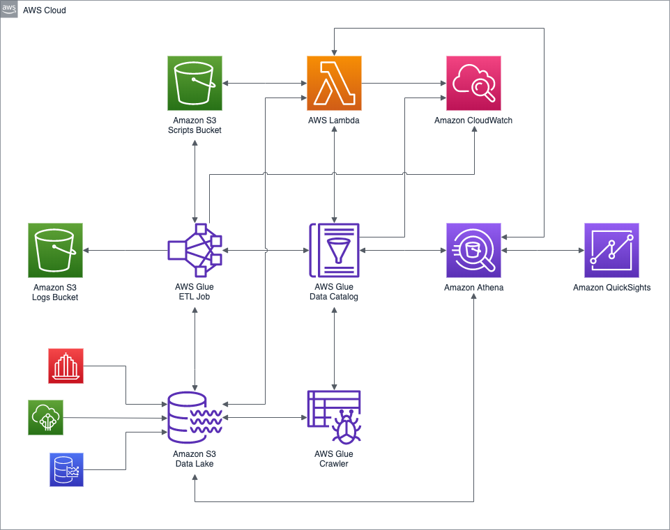 High-level AWS architecture diagram of the demonstration.
Featured Technologies
The following AWS services and open-source technologies are featured prominently in this post.

Amazon S3-based Data Lake
 An Amazon S3-based Data Lake uses Amazon S3 as its primary storage platform. Amazon S3 provides an optimal foundation for a data lake because of its virtually unlimited scalability, from gigabytes to petabytes of content. Amazon S3 provides ‘11 nines’ (99.999999999%) durability. It has scalable performance, ease-of-use features, and native encryption and access control capabilities.
AWS Glue
 AWS Glue is a fully managed extract, transform, and load (ETL) service to prepare and load data for analytics. AWS Glue discovers your data and stores the associated metadata (e.g., table definition and schema) in the AWS Glue Data Catalog. Once cataloged, your data is immediately searchable, queryable, and available for ETL.
AWS Glue Data Catalog
 The AWS Glue Data Catalog is an Apache Hive Metastore compatible, central repository to store structural and operational metadata for data assets. For a given data set, store table definition, physical location, add business-relevant attributes, as well as track how the data has changed over time.
AWS Glue Crawler
 An AWS Glue Crawler connects to a data store, progresses through a prioritized list of classifiers to extract the schema of your data and other statistics, and then populates the Glue Data Catalog with this metadata. Crawlers can run periodically to detect the availability of new data as well as changes to existing data, including table definition changes. Crawlers automatically add new tables, new partitions to an existing table, and new versions of table definitions. You can even customize Glue Crawlers to classify your own file types.
AWS Glue ETL Job
An AWS Glue ETL Job is the business logic that performs extract, transform, and load (ETL) work in AWS Glue. When you start a job, AWS Glue runs a script that extracts data from sources, transforms the data, and loads it into targets. AWS Glue generates a PySpark or Scala script, which runs on Apache Spark.
Amazon Athena
 Amazon Athena is an interactive query service that makes it easy to analyze data in Amazon S3 using standard SQL. Athena supports and works with a variety of standard data formats, including CSV, JSON, Apache ORC, Apache Avro, and Apache Parquet. Athena is integrated, out-of-the-box, with AWS Glue Data Catalog. Athena is serverless, so there is no infrastructure to manage, and you pay only for the queries that you run.
The underlying technology behind Amazon Athena is Presto, the open-source distributed SQL query engine for big data, created by Facebook. According to the AWS, the Athena query engine is based on Presto 0.172 (released April 9, 2017). In addition to Presto, Athena uses Apache Hive to define tables.
Amazon QuickSight
 Amazon QuickSight is a fully managed business intelligence (BI) service. QuickSight lets you create and publish interactive dashboards that can then be accessed from any device, and embedded into your applications, portals, and websites.
AWS Lambda
 AWS Lambda automatically runs code without requiring the provisioning or management servers. AWS Lambda automatically scales applications by running code in response to triggers. Lambda code runs in parallel. With AWS Lambda, you are charged for every 100ms your code executes and the number of times your code is triggered. You pay only for the compute time you consume.
Smart Hub Data
Everything in this post revolves around data. For the post’s demonstration, we will start with four categories of raw, synthetic data. Those data categories include Smart Hub electrical usage data, Smart Hub sensor mapping data, Smart Hub residential locations data, and electrical rate data. To demonstrate the capabilities of AWS Glue to handle multiple data formats, the four categories of raw data consist of three distinct file formats: XML, JSON, and CSV. I have attempted to incorporate as many ‘real-world’ complexities into the data without losing focus on the main subject of the post. The sample datasets are intentionally small to keep your AWS costs to a minimum for the demonstration.
To further reduce costs, we will use a variety of data partitioning schemes. According to AWS, by partitioning your data, you can restrict the amount of data scanned by each query, thus improving performance and reducing cost. We have very little data for the demonstration, in which case partitioning may negatively impact query performance. However, in a ‘real-world’ scenario, there would be millions of potential residential customers generating terabytes of data. In that case, data partitioning would be essential for both cost and performance.
Smart Hub Electrical Usage Data
The Smart Hub’s time-series electrical usage data is collected from the customer’s Smart Hub. In the demonstration’s sample electrical usage data, each row represents a completely arbitrary five-minute time interval. There are a total of ten electrical sensors whose electrical usage in kilowatt-hours (kW) is recorded and transmitted. Each Smart Hub records and transmits electrical usage for 10 device sensors, 288 times per day (24 hr / 5 min intervals), for a total of 2,880 data points per day, per Smart Hub. There are two days worth of usage data for the demonstration, for a total of 5,760 data points. The data is stored in JSON Lines format. The usage data will be partitioned in the Amazon S3-based data lake by date (e.g., ‘dt=2019-12-21’).
This file contains bidirectional Unicode text that may be interpreted or compiled differently than what appears below. To review, open the file in an editor that reveals hidden Unicode characters.
Learn more about bidirectional Unicode characters
| {"loc_id":"b6a8d42425fde548","ts":1576915200,"data":{"s_01":0,"s_02":0.00502,"s_03":0,"s_04":0,"s_05":0,"s_06":0,"s_07":0,"s_08":0,"s_09":0,"s_10":0.04167}} | |
| {"loc_id":"b6a8d42425fde548","ts":1576915500,"data":{"s_01":0,"s_02":0.00552,"s_03":0,"s_04":0,"s_05":0,"s_06":0,"s_07":0,"s_08":0,"s_09":0,"s_10":0.04147}} | |
| {"loc_id":"b6a8d42425fde548","ts":1576915800,"data":{"s_01":0.29267,"s_02":0.00642,"s_03":0,"s_04":0,"s_05":0,"s_06":0,"s_07":0,"s_08":0,"s_09":0,"s_10":0.04207}} | |
| {"loc_id":"b6a8d42425fde548","ts":1576916100,"data":{"s_01":0.29207,"s_02":0.00592,"s_03":0,"s_04":0,"s_05":0,"s_06":0,"s_07":0,"s_08":0,"s_09":0,"s_10":0.04137}} | |
| {"loc_id":"b6a8d42425fde548","ts":1576916400,"data":{"s_01":0.29217,"s_02":0.00622,"s_03":0,"s_04":0,"s_05":0,"s_06":0,"s_07":0,"s_08":0,"s_09":0,"s_10":0.04157}} | |
| {"loc_id":"b6a8d42425fde548","ts":1576916700,"data":{"s_01":0,"s_02":0.00562,"s_03":0,"s_04":0,"s_05":0,"s_06":0,"s_07":0,"s_08":0,"s_09":0,"s_10":0.04197}} | |
| {"loc_id":"b6a8d42425fde548","ts":1576917000,"data":{"s_01":0,"s_02":0.00512,"s_03":0,"s_04":0,"s_05":0,"s_06":0,"s_07":0,"s_08":0,"s_09":0,"s_10":0.04257}} | |
| {"loc_id":"b6a8d42425fde548","ts":1576917300,"data":{"s_01":0,"s_02":0.00522,"s_03":0,"s_04":0,"s_05":0,"s_06":0,"s_07":0,"s_08":0,"s_09":0,"s_10":0.04177}} | |
| {"loc_id":"b6a8d42425fde548","ts":1576917600,"data":{"s_01":0,"s_02":0.00502,"s_03":0,"s_04":0,"s_05":0,"s_06":0,"s_07":0,"s_08":0,"s_09":0,"s_10":0.04267}} | |
| {"loc_id":"b6a8d42425fde548","ts":1576917900,"data":{"s_01":0,"s_02":0.00612,"s_03":0,"s_04":0,"s_05":0,"s_06":0,"s_07":0,"s_08":0,"s_09":0,"s_10":0.04237}} |
Note the electrical usage data contains nested data. The electrical usage for each of the ten sensors is contained in a JSON array, within each time series entry. The array contains ten numeric values of type, double.
This file contains bidirectional Unicode text that may be interpreted or compiled differently than what appears below. To review, open the file in an editor that reveals hidden Unicode characters.
Learn more about bidirectional Unicode characters
| { | |
| "loc_id": "b6a8d42425fde548", | |
| "ts": 1576916400, | |
| "data": { | |
| "s_01": 0.29217, | |
| "s_02": 0.00622, | |
| "s_03": 0, | |
| "s_04": 0, | |
| "s_05": 0, | |
| "s_06": 0, | |
| "s_07": 0, | |
| "s_08": 0, | |
| "s_09": 0, | |
| "s_10": 0.04157 | |
| } | |
| } |
Real data is often complex and deeply nested. Later in the post, we will see that AWS Glue can map many common data types, including nested data objects, as illustrated below.

Smart Hub Sensor Mappings
The Smart Hub sensor mappings data maps a sensor column in the usage data (e.g., ‘s_01’ to the corresponding actual device (e.g., ‘Central Air Conditioner’). The data contains the device location, wattage, and the last time the record was modified. The data is also stored in JSON Lines format. The sensor mappings data will be partitioned in the Amazon S3-based data lake by the state of the residence (e.g., ‘state=or’ for Oregon).
This file contains bidirectional Unicode text that may be interpreted or compiled differently than what appears below. To review, open the file in an editor that reveals hidden Unicode characters.
Learn more about bidirectional Unicode characters
| {"loc_id":"b6a8d42425fde548","id":"s_01","description":"Central Air Conditioner","location":"N/A","watts":3500,"last_modified":1559347200} | |
| {"loc_id":"b6a8d42425fde548","id":"s_02","description":"Ceiling Fan","location":"Master Bedroom","watts":65,"last_modified":1559347200} | |
| {"loc_id":"b6a8d42425fde548","id":"s_03","description":"Clothes Dryer","location":"Basement","watts":5000,"last_modified":1559347200} | |
| {"loc_id":"b6a8d42425fde548","id":"s_04","description":"Clothes Washer","location":"Basement","watts":1800,"last_modified":1559347200} | |
| {"loc_id":"b6a8d42425fde548","id":"s_05","description":"Dishwasher","location":"Kitchen","watts":900,"last_modified":1559347200} | |
| {"loc_id":"b6a8d42425fde548","id":"s_06","description":"Flat Screen TV","location":"Living Room","watts":120,"last_modified":1559347200} | |
| {"loc_id":"b6a8d42425fde548","id":"s_07","description":"Microwave Oven","location":"Kitchen","watts":1000,"last_modified":1559347200} | |
| {"loc_id":"b6a8d42425fde548","id":"s_08","description":"Coffee Maker","location":"Kitchen","watts":900,"last_modified":1559347200} | |
| {"loc_id":"b6a8d42425fde548","id":"s_09","description":"Hair Dryer","location":"Master Bathroom","watts":2000,"last_modified":1559347200} | |
| {"loc_id":"b6a8d42425fde548","id":"s_10","description":"Refrigerator","location":"Kitchen","watts":500,"last_modified":1559347200} |
Smart Hub Locations
The Smart Hub locations data contains the geospatial coordinates, home address, and timezone for each residential Smart Hub. The data is stored in CSV format. The data for the four cities included in this demonstration originated from OpenAddresses, ‘the free and open global address collection.’ There are approximately 4k location records. The location data will be partitioned in the Amazon S3-based data lake by the state of the residence where the Smart Hub is installed (e.g., ‘state=or’ for Oregon).
This file contains bidirectional Unicode text that may be interpreted or compiled differently than what appears below. To review, open the file in an editor that reveals hidden Unicode characters.
Learn more about bidirectional Unicode characters
| lon | lat | number | street | unit | city | district | region | postcode | id | hash | tz | |
|---|---|---|---|---|---|---|---|---|---|---|---|---|
| -122.8077278 | 45.4715614 | 6635 | SW JUNIPER TER | 97008 | b6a8d42425fde548 | America/Los_Angeles | ||||||
| -122.8356634 | 45.4385864 | 11225 | SW PINTAIL LOOP | 97007 | 08ae3df798df8b90 | America/Los_Angeles | ||||||
| -122.8252379 | 45.4481709 | 9930 | SW WRANGLER PL | 97008 | 1c7e1f7df752663e | America/Los_Angeles | ||||||
| -122.8354211 | 45.4535977 | 9174 | SW PLATINUM PL | 97007 | b364854408ee431e | America/Los_Angeles | ||||||
| -122.8315771 | 45.4949449 | 15040 | SW MILLIKAN WAY | # 233 | 97003 | 0e97796ba31ba3b4 | America/Los_Angeles | |||||
| -122.7950339 | 45.4470259 | 10006 | SW CONESTOGA DR | # 113 | 97008 | 2b5307be5bfeb026 | America/Los_Angeles | |||||
| -122.8072836 | 45.4908594 | 12600 | SW CRESCENT ST | # 126 | 97005 | 4d74167f00f63f50 | America/Los_Angeles | |||||
| -122.8211801 | 45.4689303 | 7100 | SW 140TH PL | 97008 | c5568631f0b9de9c | America/Los_Angeles | ||||||
| -122.831154 | 45.4317057 | 15050 | SW MALLARD DR | # 101 | 97007 | dbd1321080ce9682 | America/Los_Angeles | |||||
| -122.8162856 | 45.4442878 | 10460 | SW 136TH PL | 97008 | 008faab8a9a3e519 | America/Los_Angeles |
Electrical Rates
Lastly, the electrical rate data contains the cost of electricity. In this demonstration, the assumption is that the rate varies by state, by month, and by the hour of the day. The data is stored in XML, a data export format still common to older, legacy systems. The electrical rate data will not be partitioned in the Amazon S3-based data lake.
This file contains bidirectional Unicode text that may be interpreted or compiled differently than what appears below. To review, open the file in an editor that reveals hidden Unicode characters.
Learn more about bidirectional Unicode characters
| <?xml version="1.0" encoding="UTF-8"?> | |
| <root> | |
| <row> | |
| <state>or</state> | |
| <year>2019</year> | |
| <month>12</month> | |
| <from>19:00:00</from> | |
| <to>19:59:59</to> | |
| <type>peak</type> | |
| <rate>12.623</rate> | |
| </row> | |
| <row> | |
| <state>or</state> | |
| <year>2019</year> | |
| <month>12</month> | |
| <from>20:00:00</from> | |
| <to>20:59:59</to> | |
| <type>partial-peak</type> | |
| <rate>7.232</rate> | |
| </row> | |
| <row> | |
| <state>or</state> | |
| <year>2019</year> | |
| <month>12</month> | |
| <from>21:00:00</from> | |
| <to>21:59:59</to> | |
| <type>partial-peak</type> | |
| <rate>7.232</rate> | |
| </row> | |
| <row> | |
| <state>or</state> | |
| <year>2019</year> | |
| <month>12</month> | |
| <from>22:00:00</from> | |
| <to>22:59:59</to> | |
| <type>off-peak</type> | |
| <rate>4.209</rate> | |
| </row> | |
| </root> |
Data Analysis Process
Due to the number of steps involved in the data analysis process in the demonstration, I have divided the process into four logical stages: 1) Raw Data Ingestion, 2) Data Transformation, 3) Data Enrichment, and 4) Data Visualization and Business Intelligence (BI).
 Full data analysis workflow diagram (click to enlarge…)
Raw Data Ingestion
In the Raw Data Ingestion stage, semi-structured CSV-, XML-, and JSON-format data files are copied to a secure Amazon Simple Storage Service (S3) bucket. Within the bucket, data files are organized into folders based on their physical data structure (schema). Due to the potentially unlimited number of data files, files are further organized (partitioned) into subfolders. Organizational strategies for data files are based on date, time, geographic location, customer id, or other common data characteristics.
This collection of semi-structured data files, S3 buckets, and partitions form what is referred to as a Data Lake. According to AWS, a data lake is a centralized repository that allows you to store all your structured and unstructured data at any scale.
A series of AWS Glue Crawlers process the raw CSV-, XML-, and JSON-format files, extracting metadata, and creating table definitions in the AWS Glue Data Catalog. According to AWS, an AWS Glue Data Catalog contains metadata tables, where each table specifies a single data store.

Data Transformation
In the Data Transformation stage, the raw data in the previous stage is transformed. Data transformation may include both modifying the data and changing the data format. Data modifications include data cleansing, re-casting data types, changing date formats, field-level computations, and field concatenation.
The data is then converted from CSV-, XML-, and JSON-format to Apache Parquet format and written back to the Amazon S3-based data lake. Apache Parquet is a compressed, efficient columnar storage format. Amazon Athena, like many Cloud-based services, charges you by the amount of data scanned per query. Hence, using data partitioning, bucketing, compression, and columnar storage formats, like Parquet, will reduce query cost.
Lastly, the transformed Parquet-format data is cataloged to new tables, alongside the raw CSV, XML, and JSON data, in the Glue Data Catalog.

Data Enrichment
According to ScienceDirect, data enrichment or augmentation is the process of enhancing existing information by supplementing missing or incomplete data. Typically, data enrichment is achieved by using external data sources, but that is not always the case.
Data Enrichment—the process of enhancing existing information by supplementing missing or incomplete data. –ScienceDirect
In the Data Enrichment stage, the Parquet-format Smart Hub usage data is augmented with related data from the three other data sources: sensor mappings, locations, and electrical rates. The customer’s Smart Hub usage data is enriched with the customer’s device types, the customer’s timezone, and customer’s electricity cost per monitored period based on the customer’s geographic location and time of day.

Once the data is enriched, it is converted to Parquet and optimized for query performance, stored in the data lake, and cataloged. At this point, the original CSV-, XML-, and JSON-format raw data files, the transformed Parquet-format data files, and the Parquet-format enriched data files are all stored in the Amazon S3-based data lake and cataloged in the Glue Data Catalog.

Data Visualization
In the final Data Visualization and Business Intelligence (BI) stage, the enriched data is presented and analyzed. There are many enterprise-grade services available for visualization and Business Intelligence, which integrate with Athena. Amazon services include Amazon QuickSight, Amazon EMR, and Amazon SageMaker. Third-party solutions from AWS Partners, available on the AWS Marketplace, include Tableau, Looker, Sisense, and Domo. In this demonstration, we will focus on Amazon QuickSight.
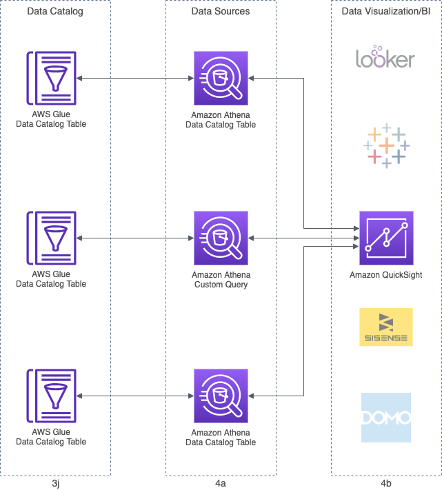
Getting Started
Requirements
To follow along with the demonstration, you will need an AWS Account and a current version of the AWS CLI. To get the most from the demonstration, you should also have Python 3 and jq installed in your work environment.
Source Code
All source code for this post can be found on GitHub. Use the following command to clone a copy of the project.
This file contains bidirectional Unicode text that may be interpreted or compiled differently than what appears below. To review, open the file in an editor that reveals hidden Unicode characters.
Learn more about bidirectional Unicode characters
| git clone \ | |
| –branch master –single-branch –depth 1 –no-tags \ | |
| https://github.com/garystafford/athena-glue-quicksight-demo.git |
Source code samples in this post are displayed as GitHub Gists, which will not display correctly on some mobile and social media browsers.
TL;DR?
Just want the jump in without reading the instructions? All the AWS CLI commands, found within the post, are consolidated in the GitHub project’s README file.
CloudFormation Stack
To start, create the ‘smart-hub-athena-glue-stack’ CloudFormation stack using the smart-hub-athena-glue.yml template. The template will create (3) Amazon S3 buckets, (1) AWS Glue Data Catalog Database, (5) Data Catalog Database Tables, (6) AWS Glue Crawlers, (1) AWS Glue ETL Job, and (1) IAM Service Role for AWS Glue.
Make sure to change the DATA_BUCKET, SCRIPT_BUCKET, and LOG_BUCKET variables, first, to your own unique S3 bucket names. I always suggest using the standard AWS 3-part convention of 1) descriptive name, 2) AWS Account ID or Account Alias, and 3) AWS Region, to name your bucket (e.g. ‘smart-hub-data-123456789012-us-east-1’).
This file contains bidirectional Unicode text that may be interpreted or compiled differently than what appears below. To review, open the file in an editor that reveals hidden Unicode characters.
Learn more about bidirectional Unicode characters
| # *** CHANGE ME *** | |
| BUCKET_SUFFIX="123456789012-us-east-1" | |
| DATA_BUCKET="smart-hub-data-${BUCKET_SUFFIX}" | |
| SCRIPT_BUCKET="smart-hub-scripts-${BUCKET_SUFFIX}" | |
| LOG_BUCKET="smart-hub-logs-${BUCKET_SUFFIX}" | |
| aws cloudformation create-stack \ | |
| –stack-name smart-hub-athena-glue-stack \ | |
| –template-body file://cloudformation/smart-hub-athena-glue.yml \ | |
| –parameters ParameterKey=DataBucketName,ParameterValue=${DATA_BUCKET} \ | |
| ParameterKey=ScriptBucketName,ParameterValue=${SCRIPT_BUCKET} \ | |
| ParameterKey=LogBucketName,ParameterValue=${LOG_BUCKET} \ | |
| –capabilities CAPABILITY_NAMED_IAM |
Raw Data Files
Next, copy the raw CSV-, XML-, and JSON-format data files from the local project to the DATA_BUCKET S3 bucket (steps 1a-1b in workflow diagram). These files represent the beginnings of the S3-based data lake. Each category of data uses a different strategy for organizing and separating the files. Note the use of the Apache Hive-style partitions (e.g., /smart_hub_data_json/dt=2019-12-21). As discussed earlier, the assumption is that the actual, large volume of data in the data lake would necessitate using partitioning to improve query performance.
This file contains bidirectional Unicode text that may be interpreted or compiled differently than what appears below. To review, open the file in an editor that reveals hidden Unicode characters.
Learn more about bidirectional Unicode characters
| # location data | |
| aws s3 cp data/locations/denver_co_1576656000.csv \ | |
| s3://${DATA_BUCKET}/smart_hub_locations_csv/state=co/ | |
| aws s3 cp data/locations/palo_alto_ca_1576742400.csv \ | |
| s3://${DATA_BUCKET}/smart_hub_locations_csv/state=ca/ | |
| aws s3 cp data/locations/portland_metro_or_1576742400.csv \ | |
| s3://${DATA_BUCKET}/smart_hub_locations_csv/state=or/ | |
| aws s3 cp data/locations/stamford_ct_1576569600.csv \ | |
| s3://${DATA_BUCKET}/smart_hub_locations_csv/state=ct/ | |
| # sensor mapping data | |
| aws s3 cp data/mappings/ \ | |
| s3://${DATA_BUCKET}/sensor_mappings_json/state=or/ \ | |
| –recursive | |
| # electrical usage data | |
| aws s3 cp data/usage/2019-12-21/ \ | |
| s3://${DATA_BUCKET}/smart_hub_data_json/dt=2019-12-21/ \ | |
| –recursive | |
| aws s3 cp data/usage/2019-12-22/ \ | |
| s3://${DATA_BUCKET}/smart_hub_data_json/dt=2019-12-22/ \ | |
| –recursive | |
| # electricity rates data | |
| aws s3 cp data/rates/ \ | |
| s3://${DATA_BUCKET}/electricity_rates_xml/ \ | |
| –recursive |
Confirm the contents of the DATA_BUCKET S3 bucket with the following command.
This file contains bidirectional Unicode text that may be interpreted or compiled differently than what appears below. To review, open the file in an editor that reveals hidden Unicode characters.
Learn more about bidirectional Unicode characters
| aws s3 ls s3://${DATA_BUCKET}/ \ | |
| –recursive –human-readable –summarize |
There should be a total of (14) raw data files in the DATA_BUCKET S3 bucket.
This file contains bidirectional Unicode text that may be interpreted or compiled differently than what appears below. To review, open the file in an editor that reveals hidden Unicode characters.
Learn more about bidirectional Unicode characters
| 2020-01-04 14:39:51 20.0 KiB electricity_rates_xml/2019_12_1575270000.xml | |
| 2020-01-04 14:39:46 1.3 KiB sensor_mappings_json/state=or/08ae3df798df8b90_1550908800.json | |
| 2020-01-04 14:39:46 1.3 KiB sensor_mappings_json/state=or/1c7e1f7df752663e_1559347200.json | |
| 2020-01-04 14:39:46 1.3 KiB sensor_mappings_json/state=or/b6a8d42425fde548_1568314800.json | |
| 2020-01-04 14:39:47 44.9 KiB smart_hub_data_json/dt=2019-12-21/08ae3df798df8b90_1576915200.json | |
| 2020-01-04 14:39:47 44.9 KiB smart_hub_data_json/dt=2019-12-21/1c7e1f7df752663e_1576915200.json | |
| 2020-01-04 14:39:47 44.9 KiB smart_hub_data_json/dt=2019-12-21/b6a8d42425fde548_1576915200.json | |
| 2020-01-04 14:39:49 44.6 KiB smart_hub_data_json/dt=2019-12-22/08ae3df798df8b90_15770016000.json | |
| 2020-01-04 14:39:49 44.6 KiB smart_hub_data_json/dt=2019-12-22/1c7e1f7df752663e_1577001600.json | |
| 2020-01-04 14:39:49 44.6 KiB smart_hub_data_json/dt=2019-12-22/b6a8d42425fde548_15770016001.json | |
| 2020-01-04 14:39:39 89.7 KiB smart_hub_locations_csv/state=ca/palo_alto_ca_1576742400.csv | |
| 2020-01-04 14:39:37 84.2 KiB smart_hub_locations_csv/state=co/denver_co_1576656000.csv | |
| 2020-01-04 14:39:44 78.6 KiB smart_hub_locations_csv/state=ct/stamford_ct_1576569600.csv | |
| 2020-01-04 14:39:42 91.6 KiB smart_hub_locations_csv/state=or/portland_metro_or_1576742400.csv | |
| Total Objects: 14 | |
| Total Size: 636.7 KiB |
Lambda Functions
Next, package the (5) Python3.8-based AWS Lambda functions for deployment.
This file contains bidirectional Unicode text that may be interpreted or compiled differently than what appears below. To review, open the file in an editor that reveals hidden Unicode characters.
Learn more about bidirectional Unicode characters
| pushd lambdas/athena-json-to-parquet-data || exit | |
| zip -r package.zip index.py | |
| popd || exit | |
| pushd lambdas/athena-csv-to-parquet-locations || exit | |
| zip -r package.zip index.py | |
| popd || exit | |
| pushd lambdas/athena-json-to-parquet-mappings || exit | |
| zip -r package.zip index.py | |
| popd || exit | |
| pushd lambdas/athena-complex-etl-query || exit | |
| zip -r package.zip index.py | |
| popd || exit | |
| pushd lambdas/athena-parquet-to-parquet-elt-data || exit | |
| zip -r package.zip index.py | |
| popd || exit |
Copy the five Lambda packages to the SCRIPT_BUCKET S3 bucket. The ZIP archive Lambda packages are accessed by the second CloudFormation stack, smart-hub-serverless. This CloudFormation stack, which creates the Lambda functions, will fail to deploy if the packages are not found in the SCRIPT_BUCKET S3 bucket.
I have chosen to place the packages in a different S3 bucket then the raw data files. In a real production environment, these two types of files would be separated, minimally, into separate buckets for security. Remember, only data should go into the data lake.
This file contains bidirectional Unicode text that may be interpreted or compiled differently than what appears below. To review, open the file in an editor that reveals hidden Unicode characters.
Learn more about bidirectional Unicode characters
| aws s3 cp lambdas/athena-json-to-parquet-data/package.zip \ | |
| s3://${SCRIPT_BUCKET}/lambdas/athena_json_to_parquet_data/ | |
| aws s3 cp lambdas/athena-csv-to-parquet-locations/package.zip \ | |
| s3://${SCRIPT_BUCKET}/lambdas/athena_csv_to_parquet_locations/ | |
| aws s3 cp lambdas/athena-json-to-parquet-mappings/package.zip \ | |
| s3://${SCRIPT_BUCKET}/lambdas/athena_json_to_parquet_mappings/ | |
| aws s3 cp lambdas/athena-complex-etl-query/package.zip \ | |
| s3://${SCRIPT_BUCKET}/lambdas/athena_complex_etl_query/ | |
| aws s3 cp lambdas/athena-parquet-to-parquet-elt-data/package.zip \ | |
| s3://${SCRIPT_BUCKET}/lambdas/athena_parquet_to_parquet_elt_data/ |
Create the second ‘smart-hub-lambda-stack’ CloudFormation stack using the smart-hub-lambda.yml CloudFormation template. The template will create (5) AWS Lambda functions and (1) Lambda execution IAM Service Role.
This file contains bidirectional Unicode text that may be interpreted or compiled differently than what appears below. To review, open the file in an editor that reveals hidden Unicode characters.
Learn more about bidirectional Unicode characters
| aws cloudformation create-stack \ | |
| –stack-name smart-hub-lambda-stack \ | |
| –template-body file://cloudformation/smart-hub-lambda.yml \ | |
| –capabilities CAPABILITY_NAMED_IAM |
At this point, we have deployed all of the AWS resources required for the demonstration using CloudFormation. We have also copied all of the raw CSV-, XML-, and JSON-format data files in the Amazon S3-based data lake.
AWS Glue Crawlers
If you recall, we created five tables in the Glue Data Catalog database as part of the CloudFormation stack. One table for each of the four raw data types and one table to hold temporary ELT data later in the demonstration. To confirm the five tables were created in the Glue Data Catalog database, use the Glue Data Catalog Console, or run the following AWS CLI / jq command.
This file contains bidirectional Unicode text that may be interpreted or compiled differently than what appears below. To review, open the file in an editor that reveals hidden Unicode characters.
Learn more about bidirectional Unicode characters
| aws glue get-tables \ | |
| –database-name smart_hub_data_catalog \ | |
| | jq -r '.TableList[].Name' |
The five data catalog tables should be as follows.
This file contains bidirectional Unicode text that may be interpreted or compiled differently than what appears below. To review, open the file in an editor that reveals hidden Unicode characters.
Learn more about bidirectional Unicode characters
| electricity_rates_xml | |
| etl_tmp_output_parquet | |
| sensor_mappings_json | |
| smart_hub_data_json | |
| smart_hub_locations_csv |
We also created six Glue Crawlers as part of the CloudFormation template. Four of these Crawlers are responsible for cataloging the raw CSV-, XML-, and JSON-format data from S3 into the corresponding, existing Glue Data Catalog database tables. The Crawlers will detect any new partitions and add those to the tables as well. Each Crawler corresponds to one of the four raw data types. Crawlers can be scheduled to run periodically, cataloging new data and updating data partitions. Crawlers will also create a Data Catalog database tables. We use Crawlers to create new tables, later in the post.
Run the four Glue Crawlers using the AWS CLI (step 1c in workflow diagram).
This file contains bidirectional Unicode text that may be interpreted or compiled differently than what appears below. To review, open the file in an editor that reveals hidden Unicode characters.
Learn more about bidirectional Unicode characters
| aws glue start-crawler –name smart-hub-locations-csv | |
| aws glue start-crawler –name smart-hub-sensor-mappings-json | |
| aws glue start-crawler –name smart-hub-data-json | |
| aws glue start-crawler –name smart-hub-rates-xml |
You can check the Glue Crawler Console to ensure the four Crawlers finished successfully.

Alternately, use another AWS CLI / jq command.
This file contains bidirectional Unicode text that may be interpreted or compiled differently than what appears below. To review, open the file in an editor that reveals hidden Unicode characters.
Learn more about bidirectional Unicode characters
| aws glue get-crawler-metrics \ | |
| | jq -r '.CrawlerMetricsList[] | "\(.CrawlerName): \(.StillEstimating), \(.TimeLeftSeconds)"' \ | |
| | grep "^smart-hub-[A-Za-z-]*" |
When complete, all Crawlers should all be in a state of ‘Still Estimating = false’ and ‘TimeLeftSeconds = 0’. In my experience, the Crawlers can take up one minute to start, after the estimation stage, and one minute to stop when complete.
This file contains bidirectional Unicode text that may be interpreted or compiled differently than what appears below. To review, open the file in an editor that reveals hidden Unicode characters.
Learn more about bidirectional Unicode characters
| smart-hub-data-json: true, 0 | |
| smart-hub-etl-tmp-output-parquet: false, 0 | |
| smart-hub-locations-csv: false, 15 | |
| smart-hub-rates-parquet: false, 0 | |
| smart-hub-rates-xml: false, 15 | |
| smart-hub-sensor-mappings-json: false, 15 |
Successfully running the four Crawlers completes the Raw Data Ingestion stage of the demonstration.
Converting to Parquet with CTAS
With the Raw Data Ingestion stage completed, we will now transform the raw Smart Hub usage data, sensor mapping data, and locations data into Parquet-format using three AWS Lambda functions. Each Lambda subsequently calls Athena, which executes a CREATE TABLE AS SELECT SQL statement (aka CTAS) . Each Lambda executes a similar command, varying only by data source, data destination, and partitioning scheme. Below, is an example of the command used for the Smart Hub electrical usage data, taken from the Python-based Lambda, athena-json-to-parquet-data/index.py.
This file contains bidirectional Unicode text that may be interpreted or compiled differently than what appears below. To review, open the file in an editor that reveals hidden Unicode characters.
Learn more about bidirectional Unicode characters
| query = \ | |
| "CREATE TABLE IF NOT EXISTS " + data_catalog + "." + output_directory + " " \ | |
| "WITH ( " \ | |
| " format = 'PARQUET', " \ | |
| " parquet_compression = 'SNAPPY', " \ | |
| " partitioned_by = ARRAY['dt'], " \ | |
| " external_location = 's3://" + data_bucket + "/" + output_directory + "' " \ | |
| ") AS " \ | |
| "SELECT * " \ | |
| "FROM " + data_catalog + "." + input_directory + ";" |
This compact, yet powerful CTAS statement converts a copy of the raw JSON- and CSV-format data files into Parquet-format, and partitions and stores the resulting files back into the S3-based data lake. Additionally, the CTAS SQL statement catalogs the Parquet-format data files into the Glue Data Catalog database, into new tables. Unfortunately, this method will not work for the XML-format raw data files, which we will tackle next.
The five deployed Lambda functions should be visible from the Lambda Console’s Functions tab.

Invoke the three Lambda functions using the AWS CLI. (part of step 2a in workflow diagram).
This file contains bidirectional Unicode text that may be interpreted or compiled differently than what appears below. To review, open the file in an editor that reveals hidden Unicode characters.
Learn more about bidirectional Unicode characters
| aws lambda invoke \ | |
| –function-name athena-json-to-parquet-data \ | |
| response.json | |
| aws lambda invoke \ | |
| –function-name athena-csv-to-parquet-locations \ | |
| response.json | |
| aws lambda invoke \ | |
| –function-name athena-json-to-parquet-mappings \ | |
| response.json |
Here is an example of the same CTAS command, shown above for the Smart Hub electrical usage data, as it is was executed successfully by Athena.
This file contains bidirectional Unicode text that may be interpreted or compiled differently than what appears below. To review, open the file in an editor that reveals hidden Unicode characters.
Learn more about bidirectional Unicode characters
| CREATE TABLE IF NOT EXISTS smart_hub_data_catalog.smart_hub_data_parquet | |
| WITH (format = 'PARQUET', | |
| parquet_compression = 'SNAPPY', | |
| partitioned_by = ARRAY['dt'], | |
| external_location = 's3://smart-hub-data-demo-account-1-us-east-1/smart_hub_data_parquet') | |
| AS | |
| SELECT * | |
| FROM smart_hub_data_catalog.smart_hub_data_json |
We can view any Athena SQL query from the Athena Console’s History tab. Clicking on a query (in pink) will copy it to the Query Editor tab and execute it. Below, we see the three SQL statements executed by the Lamba functions.
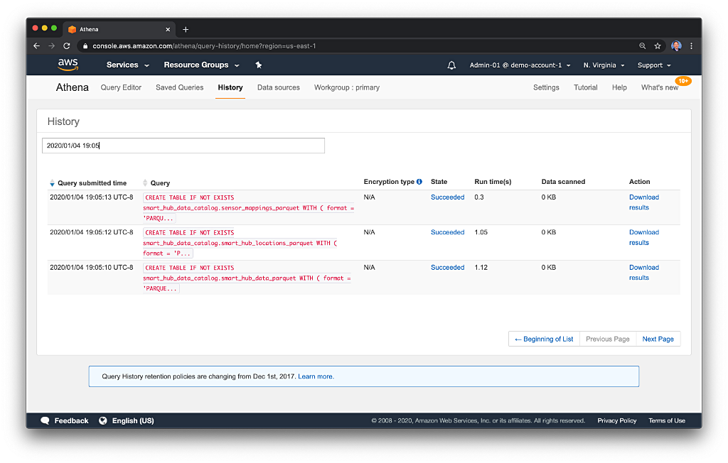
AWS Glue ETL Job for XML
If you recall, the electrical rate data is in XML format. The Lambda functions we just executed, converted the CSV and JSON data to Parquet using Athena. Currently, unlike CSV, JSON, ORC, Parquet, and Avro, Athena does not support the older XML data format. For the XML data files, we will use an AWS Glue ETL Job to convert the XML data to Parquet. The Glue ETL Job is written in Python and uses Apache Spark, along with several AWS Glue PySpark extensions. For this job, I used an existing script created in the Glue ETL Jobs Console as a base, then modified the script to meet my needs.
This file contains bidirectional Unicode text that may be interpreted or compiled differently than what appears below. To review, open the file in an editor that reveals hidden Unicode characters.
Learn more about bidirectional Unicode characters
| import sys | |
| from awsglue.transforms import * | |
| from awsglue.utils import getResolvedOptions | |
| from pyspark.context import SparkContext | |
| from awsglue.context import GlueContext | |
| from awsglue.job import Job | |
| args = getResolvedOptions(sys.argv, [ | |
| 'JOB_NAME', | |
| 's3_output_path', | |
| 'source_glue_database', | |
| 'source_glue_table' | |
| ]) | |
| s3_output_path = args['s3_output_path'] | |
| source_glue_database = args['source_glue_database'] | |
| source_glue_table = args['source_glue_table'] | |
| sc = SparkContext() | |
| glueContext = GlueContext(sc) | |
| spark = glueContext.spark_session | |
| job = Job(glueContext) | |
| job.init(args['JOB_NAME'], args) | |
| datasource0 = glueContext. \ | |
| create_dynamic_frame. \ | |
| from_catalog(database=source_glue_database, | |
| table_name=source_glue_table, | |
| transformation_ctx="datasource0") | |
| applymapping1 = ApplyMapping.apply( | |
| frame=datasource0, | |
| mappings=[("from", "string", "from", "string"), | |
| ("to", "string", "to", "string"), | |
| ("type", "string", "type", "string"), | |
| ("rate", "double", "rate", "double"), | |
| ("year", "int", "year", "int"), | |
| ("month", "int", "month", "int"), | |
| ("state", "string", "state", "string")], | |
| transformation_ctx="applymapping1") | |
| resolvechoice2 = ResolveChoice.apply( | |
| frame=applymapping1, | |
| choice="make_struct", | |
| transformation_ctx="resolvechoice2") | |
| dropnullfields3 = DropNullFields.apply( | |
| frame=resolvechoice2, | |
| transformation_ctx="dropnullfields3") | |
| datasink4 = glueContext.write_dynamic_frame.from_options( | |
| frame=dropnullfields3, | |
| connection_type="s3", | |
| connection_options={ | |
| "path": s3_output_path, | |
| "partitionKeys": ["state"] | |
| }, | |
| format="parquet", | |
| transformation_ctx="datasink4") | |
| job.commit() |
The three Python command-line arguments the script expects (lines 10–12, above) are defined in the CloudFormation template, smart-hub-athena-glue.yml. Below, we see them on lines 10–12 of the CloudFormation snippet. They are injected automatically when the job is run and can be overridden from the command line when starting the job.
This file contains bidirectional Unicode text that may be interpreted or compiled differently than what appears below. To review, open the file in an editor that reveals hidden Unicode characters.
Learn more about bidirectional Unicode characters
| GlueJobRatesToParquet: | |
| Type: AWS::Glue::Job | |
| Properties: | |
| GlueVersion: 1.0 | |
| Command: | |
| Name: glueetl | |
| PythonVersion: 3 | |
| ScriptLocation: !Sub "s3://${ScriptBucketName}/glue_scripts/rates_xml_to_parquet.py" | |
| DefaultArguments: { | |
| "–s3_output_path": !Sub "s3://${DataBucketName}/electricity_rates_parquet", | |
| "–source_glue_database": !Ref GlueDatabase, | |
| "–source_glue_table": "electricity_rates_xml", | |
| "–job-bookmark-option": "job-bookmark-enable", | |
| "–enable-spark-ui": "true", | |
| "–spark-event-logs-path": !Sub "s3://${LogBucketName}/glue-etl-jobs/" | |
| } | |
| Description: "Convert electrical rates XML data to Parquet" | |
| ExecutionProperty: | |
| MaxConcurrentRuns: 2 | |
| MaxRetries: 0 | |
| Name: rates-xml-to-parquet | |
| Role: !GetAtt "CrawlerRole.Arn" | |
| DependsOn: | |
| – CrawlerRole | |
| – GlueDatabase | |
| – DataBucket | |
| – ScriptBucket | |
| – LogBucket |
First, copy the Glue ETL Job Python script to the SCRIPT_BUCKET S3 bucket.
This file contains bidirectional Unicode text that may be interpreted or compiled differently than what appears below. To review, open the file in an editor that reveals hidden Unicode characters.
Learn more about bidirectional Unicode characters
| aws s3 cp glue-scripts/rates_xml_to_parquet.py \ | |
| s3://${SCRIPT_BUCKET}/glue_scripts/ |
Next, start the Glue ETL Job (part of step 2a in workflow diagram). Although the conversion is a relatively simple set of tasks, the creation of the Apache Spark environment, to execute the tasks, will take several minutes. Whereas the Glue Crawlers took about 2 minutes on average, the Glue ETL Job could take 10–15 minutes in my experience. The actual execution time only takes about 1–2 minutes of the 10–15 minutes to complete. In my opinion, waiting up to 15 minutes is too long to be viable for ad-hoc jobs against smaller datasets; Glue ETL Jobs are definitely targeted for big data.
This file contains bidirectional Unicode text that may be interpreted or compiled differently than what appears below. To review, open the file in an editor that reveals hidden Unicode characters.
Learn more about bidirectional Unicode characters
| aws glue start-job-run –job-name rates-xml-to-parquet |
To check on the status of the job, use the Glue ETL Jobs Console, or use the AWS CLI.
This file contains bidirectional Unicode text that may be interpreted or compiled differently than what appears below. To review, open the file in an editor that reveals hidden Unicode characters.
Learn more about bidirectional Unicode characters
| # get status of most recent job (the one that is running) | |
| aws glue get-job-run \ | |
| –job-name rates-xml-to-parquet \ | |
| –run-id "$(aws glue get-job-runs \ | |
| –job-name rates-xml-to-parquet \ | |
| | jq -r '.JobRuns[0].Id')" |
When complete, you should see results similar to the following. Note the ‘JobRunState’ is ‘SUCCEEDED.’ This particular job ran for a total of 14.92 minutes, while the actual execution time was 2.25 minutes.
This file contains bidirectional Unicode text that may be interpreted or compiled differently than what appears below. To review, open the file in an editor that reveals hidden Unicode characters.
Learn more about bidirectional Unicode characters
| { | |
| "JobRun": { | |
| "Id": "jr_f7186b26bf042ea7773ad08704d012d05299f080e7ac9b696ca8dd575f79506b", | |
| "Attempt": 0, | |
| "JobName": "rates-xml-to-parquet", | |
| "StartedOn": 1578022390.301, | |
| "LastModifiedOn": 1578023285.632, | |
| "CompletedOn": 1578023285.632, | |
| "JobRunState": "SUCCEEDED", | |
| "PredecessorRuns": [], | |
| "AllocatedCapacity": 10, | |
| "ExecutionTime": 135, | |
| "Timeout": 2880, | |
| "MaxCapacity": 10.0, | |
| "LogGroupName": "/aws-glue/jobs", | |
| "GlueVersion": "1.0" | |
| } | |
| } |
The job’s progress and the results are also visible in the AWS Glue Console’s ETL Jobs tab.

Detailed Apache Spark logs are also available in CloudWatch Management Console, which is accessible directly from the Logs link in the AWS Glue Console’s ETL Jobs tab.

The last step in the Data Transformation stage is to convert catalog the Parquet-format electrical rates data, created with the previous Glue ETL Job, using yet another Glue Crawler (part of step 2b in workflow diagram). Start the following Glue Crawler to catalog the Parquet-format electrical rates data.
This file contains bidirectional Unicode text that may be interpreted or compiled differently than what appears below. To review, open the file in an editor that reveals hidden Unicode characters.
Learn more about bidirectional Unicode characters
| aws glue start-crawler –name smart-hub-rates-parquet |
This concludes the Data Transformation stage. The raw and transformed data is in the data lake, and the following nine tables should exist in the Glue Data Catalog.
This file contains bidirectional Unicode text that may be interpreted or compiled differently than what appears below. To review, open the file in an editor that reveals hidden Unicode characters.
Learn more about bidirectional Unicode characters
| electricity_rates_parquet | |
| electricity_rates_xml | |
| etl_tmp_output_parquet | |
| sensor_mappings_json | |
| sensor_mappings_parquet | |
| smart_hub_data_json | |
| smart_hub_data_parquet | |
| smart_hub_locations_csv | |
| smart_hub_locations_parquet |
If we examine the tables, we should observe the data partitions we used to organize the data files in the Amazon S3-based data lake are contained in the table metadata. Below, we see the four partitions, based on state, of the Parquet-format locations data.

Data Enrichment
To begin the Data Enrichment stage, we will invoke the AWS Lambda, athena-complex-etl-query/index.py. This Lambda accepts input parameters (lines 28–30, below), passed in the Lambda handler’s event parameter. The arguments include the Smart Hub ID, the start date for the data requested, and the end date for the data requested. The scenario for the demonstration is that a customer with the location id value, using the electrical provider’s application, has requested data for a particular range of days (start date and end date), to visualize and analyze.
The Lambda executes a series of Athena INSERT INTO SQL statements, one statement for each of the possible Smart Hub connected electrical sensors, s_01 through s_10, for which there are values in the Smart Hub electrical usage data. Amazon just released the Amazon Athena INSERT INTO a table using the results of a SELECT query capability in September 2019, an essential addition to Athena. New Athena features are listed in the release notes.
Here, the SELECT query is actually a series of chained subqueries, using Presto SQL’s WITH clause capability. The queries join the Parquet-format Smart Hub electrical usage data sources in the S3-based data lake, with the other three Parquet-format, S3-based data sources: sensor mappings, locations, and electrical rates. The Parquet-format data is written as individual files to S3 and inserted into the existing ‘etl_tmp_output_parquet’ Glue Data Catalog database table. Compared to traditional relational database-based queries, the capabilities of Glue and Athena to enable complex SQL queries across multiple semi-structured data files, stored in S3, is truly amazing!
The capabilities of Glue and Athena to enable complex SQL queries across multiple semi-structured data files, stored in S3, is truly amazing!
Below, we see the SQL statement starting on line 43.
This file contains bidirectional Unicode text that may be interpreted or compiled differently than what appears below. To review, open the file in an editor that reveals hidden Unicode characters.
Learn more about bidirectional Unicode characters
| import boto3 | |
| import os | |
| import logging | |
| import json | |
| from typing import Dict | |
| # environment variables | |
| data_catalog = os.getenv('DATA_CATALOG') | |
| data_bucket = os.getenv('DATA_BUCKET') | |
| # variables | |
| output_directory = 'etl_tmp_output_parquet' | |
| # uses list comprehension to generate the equivalent of: | |
| # ['s_01', 's_02', …, 's_09', 's_10'] | |
| sensors = [f's_{i:02d}' for i in range(1, 11)] | |
| # logging | |
| logger = logging.getLogger() | |
| logger.setLevel(logging.INFO) | |
| # athena client | |
| athena_client = boto3.client('athena') | |
| def handler(event, context): | |
| args = { | |
| "loc_id": event['loc_id'], | |
| "date_from": event['date_from'], | |
| "date_to": event['date_to'] | |
| } | |
| athena_query(args) | |
| return { | |
| 'statusCode': 200, | |
| 'body': json.dumps("function 'athena-complex-etl-query' complete") | |
| } | |
| def athena_query(args: Dict[str, str]): | |
| for sensor in sensors: | |
| query = \ | |
| "INSERT INTO " + data_catalog + "." + output_directory + " " \ | |
| "WITH " \ | |
| " t1 AS " \ | |
| " (SELECT d.loc_id, d.ts, d.data." + sensor + " AS kwh, l.state, l.tz " \ | |
| " FROM smart_hub_data_catalog.smart_hub_data_parquet d " \ | |
| " LEFT OUTER JOIN smart_hub_data_catalog.smart_hub_locations_parquet l " \ | |
| " ON d.loc_id = l.hash " \ | |
| " WHERE d.loc_id = '" + args['loc_id'] + "' " \ | |
| " AND d.dt BETWEEN cast('" + args['date_from'] + \ | |
| "' AS date) AND cast('" + args['date_to'] + "' AS date)), " \ | |
| " t2 AS " \ | |
| " (SELECT at_timezone(from_unixtime(t1.ts, 'UTC'), t1.tz) AS ts, " \ | |
| " date_format(at_timezone(from_unixtime(t1.ts, 'UTC'), t1.tz), '%H') AS rate_period, " \ | |
| " m.description AS device, m.location, t1.loc_id, t1.state, t1.tz, t1.kwh " \ | |
| " FROM t1 LEFT OUTER JOIN smart_hub_data_catalog.sensor_mappings_parquet m " \ | |
| " ON t1.loc_id = m.loc_id " \ | |
| " WHERE t1.loc_id = '" + args['loc_id'] + "' " \ | |
| " AND m.state = t1.state " \ | |
| " AND m.description = (SELECT m2.description " \ | |
| " FROM smart_hub_data_catalog.sensor_mappings_parquet m2 " \ | |
| " WHERE m2.loc_id = '" + args['loc_id'] + "' AND m2.id = '" + sensor + "')), " \ | |
| " t3 AS " \ | |
| " (SELECT substr(r.to, 1, 2) AS rate_period, r.type, r.rate, r.year, r.month, r.state " \ | |
| " FROM smart_hub_data_catalog.electricity_rates_parquet r " \ | |
| " WHERE r.year BETWEEN cast(date_format(cast('" + args['date_from'] + \ | |
| "' AS date), '%Y') AS integer) AND cast(date_format(cast('" + args['date_to'] + \ | |
| "' AS date), '%Y') AS integer)) " \ | |
| "SELECT replace(cast(t2.ts AS VARCHAR), concat(' ', t2.tz), '') AS ts, " \ | |
| " t2.device, t2.location, t3.type, t2.kwh, t3.rate AS cents_per_kwh, " \ | |
| " round(t2.kwh * t3.rate, 4) AS cost, t2.state, t2.loc_id " \ | |
| "FROM t2 LEFT OUTER JOIN t3 " \ | |
| " ON t2.rate_period = t3.rate_period " \ | |
| "WHERE t3.state = t2.state " \ | |
| "ORDER BY t2.ts, t2.device;" | |
| logger.info(query) | |
| response = athena_client.start_query_execution( | |
| QueryString=query, | |
| QueryExecutionContext={ | |
| 'Database': data_catalog | |
| }, | |
| ResultConfiguration={ | |
| 'OutputLocation': 's3://' + data_bucket + '/tmp/' + output_directory | |
| }, | |
| WorkGroup='primary' | |
| ) | |
| logger.info(response) |
Below, is an example of one of the final queries, for the s_10 sensor, as executed by Athena. All the input parameter values, Python variables, and environment variables have been resolved into the query.
This file contains bidirectional Unicode text that may be interpreted or compiled differently than what appears below. To review, open the file in an editor that reveals hidden Unicode characters.
Learn more about bidirectional Unicode characters
| INSERT INTO smart_hub_data_catalog.etl_tmp_output_parquet | |
| WITH t1 AS (SELECT d.loc_id, d.ts, d.data.s_10 AS kwh, l.state, l.tz | |
| FROM smart_hub_data_catalog.smart_hub_data_parquet d | |
| LEFT OUTER JOIN smart_hub_data_catalog.smart_hub_locations_parquet l ON d.loc_id = l.hash | |
| WHERE d.loc_id = 'b6a8d42425fde548' | |
| AND d.dt BETWEEN cast('2019-12-21' AS date) AND cast('2019-12-22' AS date)), | |
| t2 AS (SELECT at_timezone(from_unixtime(t1.ts, 'UTC'), t1.tz) AS ts, | |
| date_format(at_timezone(from_unixtime(t1.ts, 'UTC'), t1.tz), '%H') AS rate_period, | |
| m.description AS device, | |
| m.location, | |
| t1.loc_id, | |
| t1.state, | |
| t1.tz, | |
| t1.kwh | |
| FROM t1 | |
| LEFT OUTER JOIN smart_hub_data_catalog.sensor_mappings_parquet m ON t1.loc_id = m.loc_id | |
| WHERE t1.loc_id = 'b6a8d42425fde548' | |
| AND m.state = t1.state | |
| AND m.description = (SELECT m2.description | |
| FROM smart_hub_data_catalog.sensor_mappings_parquet m2 | |
| WHERE m2.loc_id = 'b6a8d42425fde548' | |
| AND m2.id = 's_10')), | |
| t3 AS (SELECT substr(r.to, 1, 2) AS rate_period, r.type, r.rate, r.year, r.month, r.state | |
| FROM smart_hub_data_catalog.electricity_rates_parquet r | |
| WHERE r.year BETWEEN cast(date_format(cast('2019-12-21' AS date), '%Y') AS integer) | |
| AND cast(date_format(cast('2019-12-22' AS date), '%Y') AS integer)) | |
| SELECT replace(cast(t2.ts AS VARCHAR), concat(' ', t2.tz), '') AS ts, | |
| t2.device, | |
| t2.location, | |
| t3.type, | |
| t2.kwh, | |
| t3.rate AS cents_per_kwh, | |
| round(t2.kwh * t3.rate, 4) AS cost, | |
| t2.state, | |
| t2.loc_id | |
| FROM t2 | |
| LEFT OUTER JOIN t3 ON t2.rate_period = t3.rate_period | |
| WHERE t3.state = t2.state | |
| ORDER BY t2.ts, t2.device; |
Along with enriching the data, the query performs additional data transformation using the other data sources. For example, the Unix timestamp is converted to a localized timestamp containing the date and time, according to the customer’s location (line 7, above). Transforming dates and times is a frequent, often painful, data analysis task. Another example of data enrichment is the augmentation of the data with a new, computed column. The column’s values are calculated using the values of two other columns (line 33, above).
Invoke the Lambda with the following three parameters in the payload (step 3a in workflow diagram).
This file contains bidirectional Unicode text that may be interpreted or compiled differently than what appears below. To review, open the file in an editor that reveals hidden Unicode characters.
Learn more about bidirectional Unicode characters
| aws lambda invoke \ | |
| –function-name athena-complex-etl-query \ | |
| –payload "{ \"loc_id\": \"b6a8d42425fde548\", | |
| \"date_from\": \"2019-12-21\", \"date_to\": \"2019-12-22\"}" \ | |
| response.json |
The ten INSERT INTO SQL statement’s result statuses (one per device sensor) are visible from the Athena Console’s History tab.

Each Athena query execution saves that query’s results to the S3-based data lake as individual, uncompressed Parquet-format data files. The data is partitioned in the Amazon S3-based data lake by the Smart Meter location ID (e.g., ‘loc_id=b6a8d42425fde548’).
Below is a snippet of the enriched data for a customer’s clothes washer (sensor ‘s_04’). Note the timestamp is now an actual date and time in the local timezone of the customer (e.g., ‘2019-12-21 20:10:00.000’). The sensor ID (‘s_04’) is replaced with the actual device name (‘Clothes Washer’). The location of the device (‘Basement’) and the type of electrical usage period (e.g. ‘peak’ or ‘partial-peak’) has been added. Finally, the cost column has been computed.
This file contains bidirectional Unicode text that may be interpreted or compiled differently than what appears below. To review, open the file in an editor that reveals hidden Unicode characters.
Learn more about bidirectional Unicode characters
| ts | device | location | type | kwh | cents_per_kwh | cost | state | loc_id | |
|---|---|---|---|---|---|---|---|---|---|
| 2019-12-21 19:40:00.000 | Clothes Washer | Basement | peak | 0.0 | 12.623 | 0.0 | or | b6a8d42425fde548 | |
| 2019-12-21 19:45:00.000 | Clothes Washer | Basement | peak | 0.0 | 12.623 | 0.0 | or | b6a8d42425fde548 | |
| 2019-12-21 19:50:00.000 | Clothes Washer | Basement | peak | 0.1501 | 12.623 | 1.8947 | or | b6a8d42425fde548 | |
| 2019-12-21 19:55:00.000 | Clothes Washer | Basement | peak | 0.1497 | 12.623 | 1.8897 | or | b6a8d42425fde548 | |
| 2019-12-21 20:00:00.000 | Clothes Washer | Basement | partial-peak | 0.1501 | 7.232 | 1.0855 | or | b6a8d42425fde548 | |
| 2019-12-21 20:05:00.000 | Clothes Washer | Basement | partial-peak | 0.2248 | 7.232 | 1.6258 | or | b6a8d42425fde548 | |
| 2019-12-21 20:10:00.000 | Clothes Washer | Basement | partial-peak | 0.2247 | 7.232 | 1.625 | or | b6a8d42425fde548 | |
| 2019-12-21 20:15:00.000 | Clothes Washer | Basement | partial-peak | 0.2248 | 7.232 | 1.6258 | or | b6a8d42425fde548 | |
| 2019-12-21 20:20:00.000 | Clothes Washer | Basement | partial-peak | 0.2253 | 7.232 | 1.6294 | or | b6a8d42425fde548 | |
| 2019-12-21 20:25:00.000 | Clothes Washer | Basement | partial-peak | 0.151 | 7.232 | 1.092 | or | b6a8d42425fde548 |
To transform the enriched CSV-format data to Parquet-format, we need to catalog the CSV-format results using another Crawler, first (step 3d in workflow diagram).
This file contains bidirectional Unicode text that may be interpreted or compiled differently than what appears below. To review, open the file in an editor that reveals hidden Unicode characters.
Learn more about bidirectional Unicode characters
| aws glue start-crawler –name smart-hub-etl-tmp-output-parquet |
Optimizing Enriched Data
The previous step created enriched Parquet-format data. However, this data is not as optimized for query efficiency as it should be. Using the Athena INSERT INTO WITH SQL statement, allowed the data to be partitioned. However, the method does not allow the Parquet data to be easily combined into larger files and compressed. To perform both these optimizations, we will use one last Lambda, athena-parquet-to-parquet-elt-data/index.py. The Lambda will create a new location in the Amazon S3-based data lake, containing all the enriched data, in a single file and compressed using Snappy compression.
This file contains bidirectional Unicode text that may be interpreted or compiled differently than what appears below. To review, open the file in an editor that reveals hidden Unicode characters.
Learn more about bidirectional Unicode characters
| aws lambda invoke \ | |
| –function-name athena-parquet-to-parquet-elt-data \ | |
| response.json |
The resulting Parquet file is visible in the S3 Management Console.

The final step in the Data Enrichment stage is to catalog the optimized Parquet-format enriched ETL data. To catalog the data, run the following Glue Crawler (step 3i in workflow diagram
This file contains bidirectional Unicode text that may be interpreted or compiled differently than what appears below. To review, open the file in an editor that reveals hidden Unicode characters.
Learn more about bidirectional Unicode characters
| aws glue start-crawler –name smart-hub-etl-output-parquet |
Final Data Lake and Data Catalog
We should now have the following ten top-level folders of partitioned data in the S3-based data lake. The ‘tmp’ folder may be ignored.
This file contains bidirectional Unicode text that may be interpreted or compiled differently than what appears below. To review, open the file in an editor that reveals hidden Unicode characters.
Learn more about bidirectional Unicode characters
| aws s3 ls s3://${DATA_BUCKET}/ |
This file contains bidirectional Unicode text that may be interpreted or compiled differently than what appears below. To review, open the file in an editor that reveals hidden Unicode characters.
Learn more about bidirectional Unicode characters
| PRE electricity_rates_parquet/ | |
| PRE electricity_rates_xml/ | |
| PRE etl_output_parquet/ | |
| PRE etl_tmp_output_parquet/ | |
| PRE sensor_mappings_json/ | |
| PRE sensor_mappings_parquet/ | |
| PRE smart_hub_data_json/ | |
| PRE smart_hub_data_parquet/ | |
| PRE smart_hub_locations_csv/ | |
| PRE smart_hub_locations_parquet/ |
Similarly, we should now have the following ten corresponding tables in the Glue Data Catalog. Use the AWS Glue Console to confirm the tables exist.

Alternately, use the following AWS CLI / jq command to list the table names.
This file contains bidirectional Unicode text that may be interpreted or compiled differently than what appears below. To review, open the file in an editor that reveals hidden Unicode characters.
Learn more about bidirectional Unicode characters
| aws glue get-tables \ | |
| –database-name smart_hub_data_catalog \ | |
| | jq -r '.TableList[].Name' |
This file contains bidirectional Unicode text that may be interpreted or compiled differently than what appears below. To review, open the file in an editor that reveals hidden Unicode characters.
Learn more about bidirectional Unicode characters
| electricity_rates_parquet | |
| electricity_rates_xml | |
| etl_output_parquet | |
| etl_tmp_output_parquet | |
| sensor_mappings_json | |
| sensor_mappings_parquet | |
| smart_hub_data_json | |
| smart_hub_data_parquet | |
| smart_hub_locations_csv | |
| smart_hub_locations_parquet |
‘Unknown’ Bug
You may have noticed the four tables created with the AWS Lambda functions, using the CTAS SQL statement, erroneously have the ‘Classification’ of ‘Unknown’ as opposed to ‘parquet’. I am not sure why, I believe it is a possible bug with the CTAS feature. It seems to have no adverse impact on the table’s functionality. However, to fix the issue, run the following set of commands. This aws glue update-table hack will switch the table’s ‘Classification’ to ‘parquet’.
This file contains bidirectional Unicode text that may be interpreted or compiled differently than what appears below. To review, open the file in an editor that reveals hidden Unicode characters.
Learn more about bidirectional Unicode characters
| database=smart_hub_data_catalog | |
| tables=(smart_hub_locations_parquet sensor_mappings_parquet smart_hub_data_parquet etl_output_parquet) | |
| for table in ${tables}; do | |
| fixed_table=$(aws glue get-table \ | |
| –database-name "${database}" \ | |
| –name "${table}" \ | |
| | jq '.Table.Parameters.classification = "parquet" | del(.Table.DatabaseName) | del(.Table.CreateTime) | del(.Table.UpdateTime) | del(.Table.CreatedBy) | del(.Table.IsRegisteredWithLakeFormation)') | |
| fixed_table=$(echo ${fixed_table} | jq .Table) | |
| aws glue update-table \ | |
| –database-name "${database}" \ | |
| –table-input "${fixed_table}" | |
| echo "table '${table}' classification changed to 'parquet'" | |
| done |
The results of the fix may be seen from the AWS Glue Console. All ten tables are now classified correctly.

Explore the Data
Before starting to visualize and analyze the data with Amazon QuickSight, try executing a few Athena queries against the tables in the Glue Data Catalog database, using the Athena Query Editor. Working in the Editor is the best way to understand the data, learn Athena, and debug SQL statements and queries. The Athena Query Editor has convenient developer features like SQL auto-complete and query formatting capabilities.
Be mindful when writing queries and searching the Internet for SQL references, the Athena query engine is based on Presto 0.172. The current version of Presto, 0.229, is more than 50 releases ahead of the current Athena version. Both Athena and Presto functionality has changed and diverged. There are additional considerations and limitations for SQL queries in Athena to be aware of.

Here are a few simple, ad-hoc queries to run in the Athena Query Editor.
This file contains bidirectional Unicode text that may be interpreted or compiled differently than what appears below. To review, open the file in an editor that reveals hidden Unicode characters.
Learn more about bidirectional Unicode characters
| — preview the final etl data | |
| SELECT * | |
| FROM smart_hub_data_catalog.etl_output_parquet | |
| LIMIT 10; | |
| — total cost in $'s for each device, at location 'b6a8d42425fde548' | |
| — from high to low, on December 21, 2019 | |
| SELECT device, | |
| concat('$', cast(cast(sum(cost) / 100 AS decimal(10, 2)) AS varchar)) AS total_cost | |
| FROM smart_hub_data_catalog.etl_tmp_output_parquet | |
| WHERE loc_id = 'b6a8d42425fde548' | |
| AND date (cast(ts AS timestamp)) = date '2019-12-21' | |
| GROUP BY device | |
| ORDER BY total_cost DESC; | |
| — count of smart hub residential locations in Oregon and California, | |
| — grouped by zip code, sorted by count | |
| SELECT DISTINCT postcode, upper(state), count(postcode) AS smart_hub_count | |
| FROM smart_hub_data_catalog.smart_hub_locations_parquet | |
| WHERE state IN ('or', 'ca') | |
| AND length(cast(postcode AS varchar)) >= 5 | |
| GROUP BY state, postcode | |
| ORDER BY smart_hub_count DESC, postcode; | |
| — electrical usage for the clothes washer | |
| — over a 30-minute period, on December 21, 2019 | |
| SELECT ts, device, location, type, cost | |
| FROM smart_hub_data_catalog.etl_tmp_output_parquet | |
| WHERE loc_id = 'b6a8d42425fde548' | |
| AND device = 'Clothes Washer' | |
| AND cast(ts AS timestamp) | |
| BETWEEN timestamp '2019-12-21 08:45:00' | |
| AND timestamp '2019-12-21 09:15:00' | |
| ORDER BY ts; |
Cleaning Up
You may choose to save the AWS resources created in part one of this demonstration, to be used in part two. Since you are not actively running queries against the data, ongoing AWS costs will be minimal. If you eventually choose to clean up the AWS resources created in part one of this demonstration, execute the following AWS CLI commands. To avoid failures, make sure each command completes before running the subsequent command. You will need to confirm the CloudFormation stacks are deleted using the AWS CloudFormation Console or the AWS CLI. These commands will not remove Amazon QuickSight data sets, analyses, and dashboards created in part two. However, deleting the AWS Glue Data Catalog and the underlying data sources will impact the ability to visualize the data in QuickSight.
This file contains bidirectional Unicode text that may be interpreted or compiled differently than what appears below. To review, open the file in an editor that reveals hidden Unicode characters.
Learn more about bidirectional Unicode characters
| # delete s3 contents first | |
| aws s3 rm s3://${DATA_BUCKET} –recursive | |
| aws s3 rm s3://${SCRIPT_BUCKET} –recursive | |
| aws s3 rm s3://${LOG_BUCKET} –recursive | |
| # then, delete lambda cfn stack | |
| aws cloudformation delete-stack –stack-name smart-hub-lambda-stack | |
| # finally, delete athena-glue-s3 stack | |
| aws cloudformation delete-stack –stack-name smart-hub-athena-glue-stack |
Part Two
In part one, starting with raw, semi-structured data in multiple formats, we learned how to ingest, transform, and enrich that data using Amazon S3, AWS Glue, Amazon Athena, and AWS Lambda. We built an S3-based data lake and learned how AWS leverages open-source technologies, including Presto, Apache Hive, and Apache Parquet. In part two of this post, we will use the transformed and enriched datasets, stored in the data lake, to create compelling visualizations using Amazon QuickSight.
All opinions expressed in this post are my own and not necessarily the views of my current or past employers or their clients.
Getting Started with Data Analytics using Jupyter Notebooks, PySpark, and Docker
Posted by Gary A. Stafford in Bash Scripting, Big Data, Build Automation, DevOps, Python, Software Development on December 6, 2019
There is little question, big data analytics, data science, artificial intelligence (AI), and machine learning (ML), a subcategory of AI, have all experienced a tremendous surge in popularity over the last few years. Behind the marketing hype, these technologies are having a significant influence on many aspects of our modern lives. Due to their popularity and potential benefits, commercial enterprises, academic institutions, and the public sector are rushing to develop hardware and software solutions to lower the barriers to entry and increase the velocity of ML and Data Scientists and Engineers.

(courtesy Google Trends and Plotly)
Many open-source software projects are also lowering the barriers to entry into these technologies. An excellent example of one such open-source project working on this challenge is Project Jupyter. Similar to Apache Zeppelin and the newly open-sourced Netflix’s Polynote, Jupyter Notebooks enables data-driven, interactive, and collaborative data analytics.
This post will demonstrate the creation of a containerized data analytics environment using Jupyter Docker Stacks. The particular environment will be suited for learning and developing applications for Apache Spark using the Python, Scala, and R programming languages. We will focus on Python and Spark, using PySpark.
Featured Technologies
The following technologies are featured prominently in this post.
Jupyter Notebooks
According to Project Jupyter, the Jupyter Notebook, formerly known as the IPython Notebook, is an open-source web application that allows users to create and share documents that contain live code, equations, visualizations, and narrative text. Uses include data cleansing and transformation, numerical simulation, statistical modeling, data visualization, machine learning, and much more. The word, Jupyter, is a loose acronym for Julia, Python, and R, but today, Jupyter supports many programming languages.
Interest in Jupyter Notebooks has grown dramatically over the last 3–5 years, fueled in part by the major Cloud providers, AWS, Google Cloud, and Azure. Amazon Sagemaker, Amazon EMR (Elastic MapReduce), Google Cloud Dataproc, Google Colab (Collaboratory), and Microsoft Azure Notebooks all have direct integrations with Jupyter notebooks for big data analytics and machine learning.

(courtesy Google Trends and Plotly)
Jupyter Docker Stacks
To enable quick and easy access to Jupyter Notebooks, Project Jupyter has created Jupyter Docker Stacks. The stacks are ready-to-run Docker images containing Jupyter applications, along with accompanying technologies. Currently, the Jupyter Docker Stacks focus on a variety of specializations, including the r-notebook, scipy-notebook, tensorflow-notebook, datascience-notebook, pyspark-notebook, and the subject of this post, the all-spark-notebook. The stacks include a wide variety of well-known packages to extend their functionality, such as scikit-learn, pandas, Matplotlib, Bokeh, NumPy, and Facets.
Apache Spark
According to Apache, Spark is a unified analytics engine for large-scale data processing. Starting as a research project at the UC Berkeley AMPLab in 2009, Spark was open-sourced in early 2010 and moved to the Apache Software Foundation in 2013. Reviewing the postings on any major career site will confirm that Spark is widely used by well-known modern enterprises, such as Netflix, Adobe, Capital One, Lockheed Martin, JetBlue Airways, Visa, and Databricks. At the time of this post, LinkedIn, alone, had approximately 3,500 listings for jobs that reference the use of Apache Spark, just in the United States.
With speeds up to 100 times faster than Hadoop, Apache Spark achieves high performance for static, batch, and streaming data, using a state-of-the-art DAG (Directed Acyclic Graph) scheduler, a query optimizer, and a physical execution engine. Spark’s polyglot programming model allows users to write applications quickly in Scala, Java, Python, R, and SQL. Spark includes libraries for Spark SQL (DataFrames and Datasets), MLlib (Machine Learning), GraphX (Graph Processing), and DStreams (Spark Streaming). You can run Spark using its standalone cluster mode, Apache Hadoop YARN, Mesos, or Kubernetes.
PySpark
The Spark Python API, PySpark, exposes the Spark programming model to Python. PySpark is built on top of Spark’s Java API and uses Py4J. According to Apache, Py4J, a bridge between Python and Java, enables Python programs running in a Python interpreter to dynamically access Java objects in a Java Virtual Machine (JVM). Data is processed in Python and cached and shuffled in the JVM.
Docker
According to Docker, their technology gives developers and IT the freedom to build, manage, and secure business-critical applications without the fear of technology or infrastructure lock-in. For this post, I am using the current stable version of Docker Desktop Community version for macOS, as of March 2020.

Docker Swarm
Current versions of Docker include both a Kubernetes and Swarm orchestrator for deploying and managing containers. We will choose Swarm for this demonstration. According to Docker, the cluster management and orchestration features embedded in the Docker Engine are built using swarmkit. Swarmkit is a separate project that implements Docker’s orchestration layer and is used directly within Docker.
PostgreSQL
PostgreSQL is a powerful, open-source, object-relational database system. According to their website, PostgreSQL comes with many features aimed to help developers build applications, administrators to protect data integrity and build fault-tolerant environments, and help manage data no matter how big or small the dataset.
Demonstration
In this demonstration, we will explore the capabilities of the Spark Jupyter Docker Stack to provide an effective data analytics development environment. We will explore a few everyday uses, including executing Python scripts, submitting PySpark jobs, and working with Jupyter Notebooks, and reading and writing data to and from different file formats and a database. We will be using the latest jupyter/all-spark-notebook Docker Image. This image includes Python, R, and Scala support for Apache Spark, using Apache Toree.
Architecture
As shown below, we will deploy a Docker stack to a single-node Docker swarm. The stack consists of a Jupyter All-Spark-Notebook, PostgreSQL (Alpine Linux version 12), and Adminer container. The Docker stack will have two local directories bind-mounted into the containers. Files from our GitHub project will be shared with the Jupyter application container through a bind-mounted directory. Our PostgreSQL data will also be persisted through a bind-mounted directory. This allows us to persist data external to the ephemeral containers. If the containers are restarted or recreated, the data is preserved locally.
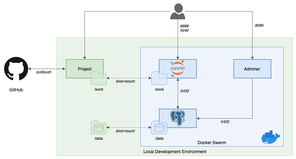
Source Code
All source code for this post can be found on GitHub. Use the following command to clone the project. Note this post uses the v2 branch.
git clone \
  --branch v2 --single-branch --depth 1 --no-tags \
  https://github.com/garystafford/pyspark-setup-demo.git
Source code samples are displayed as GitHub Gists, which may not display correctly on some mobile and social media browsers.
Deploy Docker Stack
To start, create the $HOME/data/postgres directory to store PostgreSQL data files.
mkdir -p ~/data/postgres
This directory will be bind-mounted into the PostgreSQL container on line 41 of the stack.yml file, $HOME/data/postgres:/var/lib/postgresql/data. The HOME environment variable assumes you are working on Linux or macOS and is equivalent to HOMEPATH on Windows.
The Jupyter container’s working directory is set on line 15 of the stack.yml file, working_dir: /home/$USER/work. The local bind-mounted working directory is $PWD/work. This path is bind-mounted to the working directory in the Jupyter container, on line 29 of the Docker stack file, $PWD/work:/home/$USER/work. The PWD environment variable assumes you are working on Linux or macOS (CD on Windows).
By default, the user within the Jupyter container is jovyan. We will override that user with our own local host’s user account, as shown on line 21 of the Docker stack file, NB_USER: $USER. We will use the host’s USER environment variable value (equivalent to USERNAME on Windows). There are additional options for configuring the Jupyter container. Several of those options are used on lines 17–22 of the Docker stack file (gist).
This file contains bidirectional Unicode text that may be interpreted or compiled differently than what appears below. To review, open the file in an editor that reveals hidden Unicode characters.
Learn more about bidirectional Unicode characters
| # docker stack deploy -c stack.yml jupyter | |
| # optional pgadmin container | |
| version: "3.7" | |
| networks: | |
| demo-net: | |
| services: | |
| spark: | |
| image: jupyter/all-spark-notebook:latest | |
| ports: | |
| – "8888:8888/tcp" | |
| – "4040:4040/tcp" | |
| networks: | |
| – demo-net | |
| working_dir: /home/$USER/work | |
| environment: | |
| CHOWN_HOME: "yes" | |
| GRANT_SUDO: "yes" | |
| NB_UID: 1000 | |
| NB_GID: 100 | |
| NB_USER: $USER | |
| NB_GROUP: staff | |
| user: root | |
| deploy: | |
| replicas: 1 | |
| restart_policy: | |
| condition: on-failure | |
| volumes: | |
| – $PWD/work:/home/$USER/work | |
| postgres: | |
| image: postgres:12-alpine | |
| environment: | |
| POSTGRES_USERNAME: postgres | |
| POSTGRES_PASSWORD: postgres1234 | |
| POSTGRES_DB: bakery | |
| ports: | |
| – "5432:5432/tcp" | |
| networks: | |
| – demo-net | |
| volumes: | |
| – $HOME/data/postgres:/var/lib/postgresql/data | |
| deploy: | |
| restart_policy: | |
| condition: on-failure | |
| adminer: | |
| image: adminer:latest | |
| ports: | |
| – "8080:8080/tcp" | |
| networks: | |
| – demo-net | |
| deploy: | |
| restart_policy: | |
| condition: on-failure | |
| # pgadmin: | |
| # image: dpage/pgadmin4:latest | |
| # environment: | |
| # PGADMIN_DEFAULT_EMAIL: user@domain.com | |
| # PGADMIN_DEFAULT_PASSWORD: 5up3rS3cr3t! | |
| # ports: | |
| # – "8180:80/tcp" | |
| # networks: | |
| # – demo-net | |
| # deploy: | |
| # restart_policy: | |
| # condition: on-failure |
The jupyter/all-spark-notebook Docker image is large, approximately 5 GB. Depending on your Internet connection, if this is the first time you have pulled this image, the stack may take several minutes to enter a running state. Although not required, I usually pull new Docker images in advance.
docker pull jupyter/all-spark-notebook:latest
docker pull postgres:12-alpine
docker pull adminer:latest
Assuming you have a recent version of Docker installed on your local development machine and running in swarm mode, standing up the stack is as easy as running the following docker command from the root directory of the project.
docker stack deploy -c stack.yml jupyter
The Docker stack consists of a new overlay network, jupyter_demo-net, and three containers. To confirm the stack deployed successfully, run the following docker command.
docker stack ps jupyter --no-trunc

To access the Jupyter Notebook application, you need to obtain the Jupyter URL and access token. The Jupyter URL and the access token are output to the Jupyter container log, which can be accessed with the following command.
docker logs $(docker ps | grep jupyter_spark | awk '{print $NF}')
You should observe log output similar to the following. Retrieve the complete URL, for example, http://127.0.0.1:8888/?token=f78cbe..., to access the Jupyter web-based user interface.

From the Jupyter dashboard landing page, you should see all the files in the project’s work/ directory. Note the types of files you can create from the dashboard, including Python 3, R, and Scala (using Apache Toree or spylon-kernal) notebooks, and text. You can also open a Jupyter terminal or create a new Folder from the drop-down menu. At the time of this post (March 2020), the latest jupyter/all-spark-notebook Docker Image runs Spark 2.4.5, Scala 2.11.12, Python 3.7.6, and OpenJDK 64-Bit Server VM, Java 1.8.0 Update 242.

Bootstrap Environment
Included in the project is a bootstrap script, bootstrap_jupyter.sh. The script will install the required Python packages using pip, the Python package installer, and a requirement.txt file. The bootstrap script also installs the latest PostgreSQL driver JAR, configures Apache Log4j to reduce log verbosity when submitting Spark jobs, and installs htop. Although these tasks could also be done from a Jupyter terminal or from within a Jupyter notebook, using a bootstrap script ensures you will have a consistent work environment every time you spin up the Jupyter Docker stack. Add or remove items from the bootstrap script as necessary.
This file contains bidirectional Unicode text that may be interpreted or compiled differently than what appears below. To review, open the file in an editor that reveals hidden Unicode characters.
Learn more about bidirectional Unicode characters
| #!/bin/bash | |
| set -ex | |
| # update/upgrade and install htop | |
| sudo apt-get update -y && sudo apt-get upgrade -y | |
| sudo apt-get install htop | |
| # install required python packages | |
| python3 -m pip install –user –upgrade pip | |
| python3 -m pip install -r requirements.txt –upgrade | |
| # download latest postgres driver jar | |
| POSTGRES_JAR="postgresql-42.2.17.jar" | |
| if [ -f "$POSTGRES_JAR" ]; then | |
| echo "$POSTGRES_JAR exist" | |
| else | |
| wget -nv "https://jdbc.postgresql.org/download/${POSTGRES_JAR}" | |
| fi | |
| # spark-submit logging level from INFO to WARN | |
| sudo cp log4j.properties /usr/local/spark/conf/log4j.properties |
That’s it, our new Jupyter environment is ready to start exploring.
Running Python Scripts
One of the simplest tasks we could perform in our new Jupyter environment is running Python scripts. Instead of worrying about installing and maintaining the correct versions of Python and multiple Python packages on your own development machine, we can run Python scripts from within the Jupyter container. At the time of this post update, the latest jupyter/all-spark-notebook Docker image runs Python 3.7.3 and Conda 4.7.12. Let’s start with a simple Python script, 01_simple_script.py.
This file contains bidirectional Unicode text that may be interpreted or compiled differently than what appears below. To review, open the file in an editor that reveals hidden Unicode characters.
Learn more about bidirectional Unicode characters
| #!/usr/bin/python3 | |
| import random | |
| technologies = [ | |
| 'PySpark', 'Python', 'Spark', 'Scala', 'Java', 'Project Jupyter', 'R' | |
| ] | |
| print("Technologies: %s\n" % technologies) | |
| technologies.sort() | |
| print("Sorted: %s\n" % technologies) | |
| print("I'm interested in learning about %s." % random.choice(technologies)) |
From a Jupyter terminal window, use the following command to run the script.
python3 01_simple_script.py
You should observe the following output.

Kaggle Datasets
To explore more features of the Jupyter and PySpark, we will use a publicly available dataset from Kaggle. Kaggle is an excellent open-source resource for datasets used for big-data and ML projects. Their tagline is ‘Kaggle is the place to do data science projects’. For this demonstration, we will use the Transactions from a bakery dataset from Kaggle. The dataset is available as a single CSV-format file. A copy is also included in the project.

The ‘Transactions from a bakery’ dataset contains 21,294 rows with 4 columns of data. Although certainly not big data, the dataset is large enough to test out the Spark Jupyter Docker Stack functionality. The data consists of 9,531 customer transactions for 21,294 bakery items between 2016-10-30 and 2017-04-09 (gist).
This file contains bidirectional Unicode text that may be interpreted or compiled differently than what appears below. To review, open the file in an editor that reveals hidden Unicode characters.
Learn more about bidirectional Unicode characters
| Date | Time | Transaction | Item | |
|---|---|---|---|---|
| 2016-10-30 | 09:58:11 | 1 | Bread | |
| 2016-10-30 | 10:05:34 | 2 | Scandinavian | |
| 2016-10-30 | 10:05:34 | 2 | Scandinavian | |
| 2016-10-30 | 10:07:57 | 3 | Hot chocolate | |
| 2016-10-30 | 10:07:57 | 3 | Jam | |
| 2016-10-30 | 10:07:57 | 3 | Cookies | |
| 2016-10-30 | 10:08:41 | 4 | Muffin | |
| 2016-10-30 | 10:13:03 | 5 | Coffee | |
| 2016-10-30 | 10:13:03 | 5 | Pastry | |
| 2016-10-30 | 10:13:03 | 5 | Bread |
Submitting Spark Jobs
We are not limited to Jupyter notebooks to interact with Spark. We can also submit scripts directly to Spark from the Jupyter terminal. This is typically how Spark is used in a Production for performing analysis on large datasets, often on a regular schedule, using tools such as Apache Airflow. With Spark, you are load data from one or more data sources. After performing operations and transformations on the data, the data is persisted to a datastore, such as a file or a database, or conveyed to another system for further processing.
The project includes a simple Python PySpark ETL script, 02_pyspark_job.py. The ETL script loads the original Kaggle Bakery dataset from the CSV file into memory, into a Spark DataFrame. The script then performs a simple Spark SQL query, calculating the total quantity of each type of bakery item sold, sorted in descending order. Finally, the script writes the results of the query to a new CSV file, output/items-sold.csv.
This file contains bidirectional Unicode text that may be interpreted or compiled differently than what appears below. To review, open the file in an editor that reveals hidden Unicode characters.
Learn more about bidirectional Unicode characters
| #!/usr/bin/python3 | |
| from pyspark.sql import SparkSession | |
| spark = SparkSession \ | |
| .builder \ | |
| .appName('spark-demo') \ | |
| .getOrCreate() | |
| df_bakery = spark.read \ | |
| .format('csv') \ | |
| .option('header', 'true') \ | |
| .option('delimiter', ',') \ | |
| .option('inferSchema', 'true') \ | |
| .load('BreadBasket_DMS.csv') | |
| df_sorted = df_bakery.cube('item').count() \ | |
| .filter('item NOT LIKE \'NONE\'') \ | |
| .filter('item NOT LIKE \'Adjustment\'') \ | |
| .orderBy(['count', 'item'], ascending=[False, True]) | |
| df_sorted.show(10, False) | |
| df_sorted.coalesce(1) \ | |
| .write.format('csv') \ | |
| .option('header', 'true') \ | |
| .save('output/items-sold.csv', mode='overwrite') |
Run the script directly from a Jupyter terminal using the following command.
python3 02_pyspark_job.py
An example of the output of the Spark job is shown below.

Typically, you would submit the Spark job using the spark-submit command. Use a Jupyter terminal to run the following command.
$SPARK_HOME/bin/spark-submit 02_pyspark_job.py
Below, we see the output from the spark-submit command. Printing the results in the output is merely for the purposes of the demo. Typically, Spark jobs are submitted non-interactively, and the results are persisted directly to a datastore or conveyed to another system.
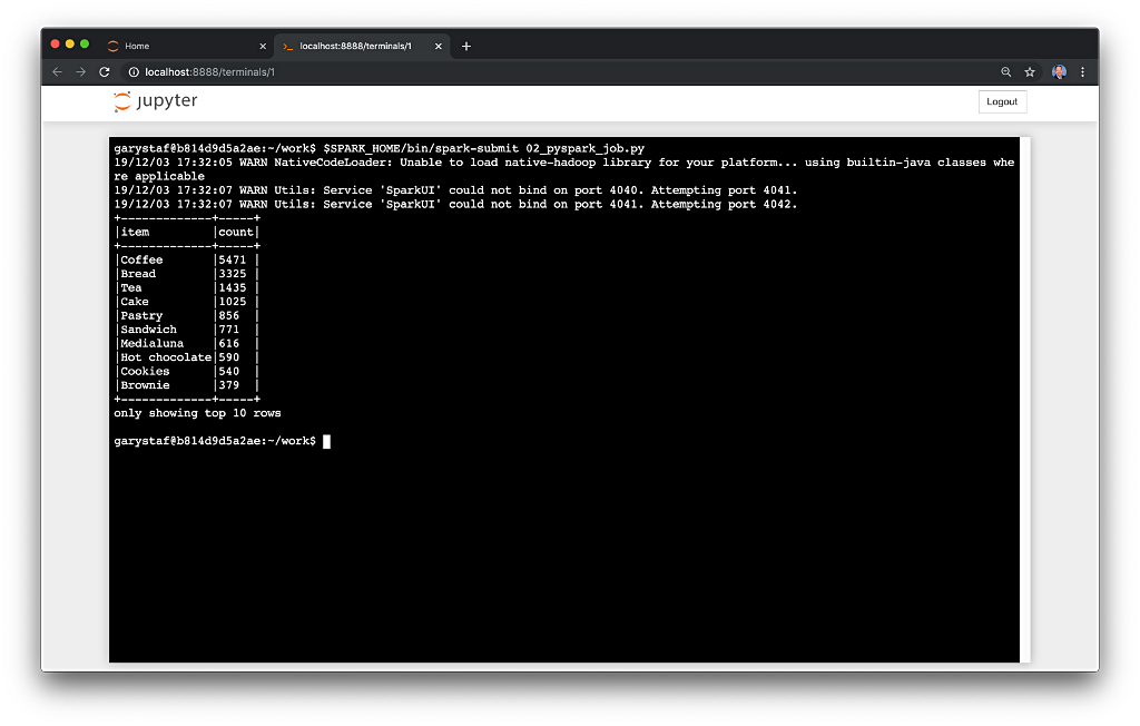
Using the following commands, we can view the resulting CVS file, created by the spark job.
ls -alh output/items-sold.csv/
head -5 output/items-sold.csv/*.csv
An example of the files created by the spark job is shown below. We should have discovered that coffee is the most commonly sold bakery item with 5,471 sales, followed by bread with 3,325 sales.

Interacting with Databases
To demonstrate the flexibility of Jupyter to work with databases, PostgreSQL is part of the Docker Stack. We can read and write data from the Jupyter container to the PostgreSQL instance, running in a separate container. To begin, we will run a SQL script, written in Python, to create our database schema and some test data in a new database table. To do so, we will use the psycopg2, the PostgreSQL database adapter package for the Python, we previously installed into our Jupyter container using the bootstrap script. The below Python script, 03_load_sql.py, will execute a set of SQL statements contained in a SQL file, bakery.sql, against the PostgreSQL container instance.
This file contains bidirectional Unicode text that may be interpreted or compiled differently than what appears below. To review, open the file in an editor that reveals hidden Unicode characters.
Learn more about bidirectional Unicode characters
| #!/usr/bin/python3 | |
| import psycopg2 | |
| # connect to database | |
| connect_str = 'host=postgres port=5432 dbname=bakery user=postgres password=postgres1234' | |
| conn = psycopg2.connect(connect_str) | |
| conn.autocommit = True | |
| cursor = conn.cursor() | |
| # execute sql script | |
| sql_file = open('bakery.sql', 'r') | |
| sqlFile = sql_file.read() | |
| sql_file.close() | |
| sqlCommands = sqlFile.split(';') | |
| for command in sqlCommands: | |
| print(command) | |
| if command.strip() != '': | |
| cursor.execute(command) | |
| # import data from csv file | |
| with open('BreadBasket_DMS.csv', 'r') as f: | |
| next(f) # Skip the header row. | |
| cursor.copy_from( | |
| f, | |
| 'transactions', | |
| sep=',', | |
| columns=('date', 'time', 'transaction', 'item') | |
| ) | |
| conn.commit() | |
| # confirm by selecting record | |
| command = 'SELECT COUNT(*) FROM public.transactions;' | |
| cursor.execute(command) | |
| recs = cursor.fetchall() | |
| print('Row count: %d' % recs[0]) |
The SQL file, bakery.sql.
This file contains bidirectional Unicode text that may be interpreted or compiled differently than what appears below. To review, open the file in an editor that reveals hidden Unicode characters.
Learn more about bidirectional Unicode characters
| DROP TABLE IF EXISTS "transactions"; | |
| DROP SEQUENCE IF EXISTS transactions_id_seq; | |
| CREATE SEQUENCE transactions_id_seq INCREMENT 1 MINVALUE 1 MAXVALUE 2147483647 START 1 CACHE 1; | |
| CREATE TABLE "public"."transactions" | |
| ( | |
| "id" integer DEFAULT nextval('transactions_id_seq') NOT NULL, | |
| "date" character varying(10) NOT NULL, | |
| "time" character varying(8) NOT NULL, | |
| "transaction" integer NOT NULL, | |
| "item" character varying(50) NOT NULL | |
| ) WITH (oids = false); |
To execute the script, run the following command.
python3 03_load_sql.py
This should result in the following output, if successful.

Adminer
To confirm the SQL script’s success, use Adminer. Adminer (formerly phpMinAdmin) is a full-featured database management tool written in PHP. Adminer natively recognizes PostgreSQL, MySQL, SQLite, and MongoDB, among other database engines. The current version is 4.7.6 (March 2020).
Adminer should be available on localhost port 8080. The password credentials, shown below, are located in the stack.yml file. The server name, postgres, is the name of the PostgreSQL Docker container. This is the domain name the Jupyter container will use to communicate with the PostgreSQL container.
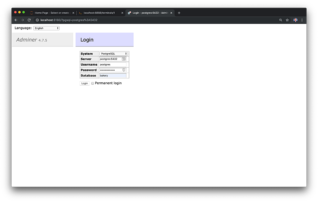
Connecting to the new bakery database with Adminer, we should see the transactions table.

The table should contain 21,293 rows, each with 5 columns of data.

pgAdmin
Another excellent choice for interacting with PostgreSQL, in particular, is pgAdmin 4. It is my favorite tool for the administration of PostgreSQL. Although limited to PostgreSQL, the user interface and administrative capabilities of pgAdmin is superior to Adminer, in my opinion. For brevity, I chose not to include pgAdmin in this post. The Docker stack also contains a pgAdmin container, which has been commented out. To use pgAdmin, just uncomment the container and re-run the Docker stack deploy command. pgAdmin should then be available on localhost port 81. The pgAdmin login credentials are in the Docker stack file.


Developing Jupyter Notebooks
The real power of the Jupyter Docker Stacks containers is Jupyter Notebooks. According to the Jupyter Project, the notebook extends the console-based approach to interactive computing in a qualitatively new direction, providing a web-based application suitable for capturing the whole computation process, including developing, documenting, and executing code, as well as communicating the results. Notebook documents contain the inputs and outputs of an interactive session as well as additional text that accompanies the code but is not meant for execution.
To explore the capabilities of Jupyter notebooks, the project includes two simple Jupyter notebooks. The first notebooks, 04_notebook.ipynb, demonstrates typical PySpark functions, such as loading data from a CSV file and from the PostgreSQL database, performing basic data analysis with Spark SQL including the use of PySpark user-defined functions (UDF), graphing the data using BokehJS, and finally, saving data back to the database, as well as to the fast and efficient Apache Parquet file format. Below we see several notebook cells demonstrating these features.
IDE Integration
Recall, the working directory, containing the GitHub source code for the project, is bind-mounted to the Jupyter container. Therefore, you can also edit any of the files, including notebooks, in your favorite IDE, such as JetBrains PyCharm and Microsoft Visual Studio Code. PyCharm has built-in language support for Jupyter Notebooks, as shown below.

As does Visual Studio Code using the Python extension.
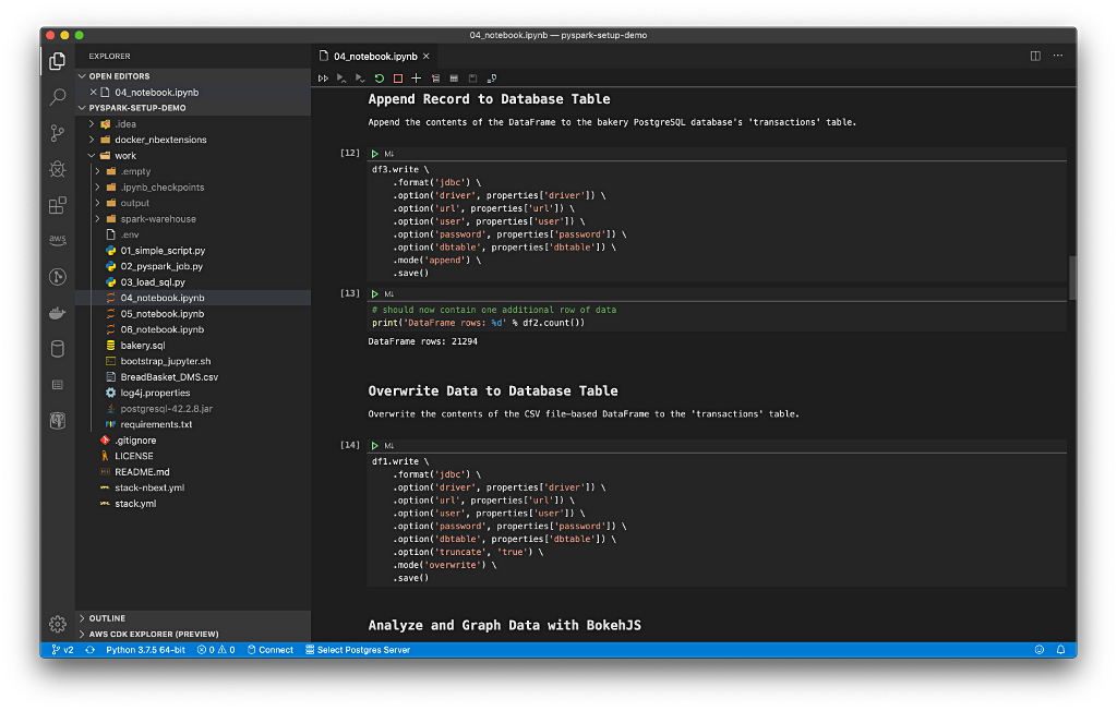
Using Additional Packages
As mentioned in the Introduction, the Jupyter Docker Stacks come ready-to-run, with a wide variety of Python packages to extend their functionality. To demonstrate the use of these packages, the project contains a second Jupyter notebook document, 05_notebook.ipynb. This notebook uses SciPy, the well-known Python package for mathematics, science, and engineering, NumPy, the well-known Python package for scientific computing, and the Plotly Python Graphing Library. While NumPy and SciPy are included on the Jupyter Docker Image, the bootstrap script uses pip to install the required Plotly packages. Similar to Bokeh, shown in the previous notebook, we can use these libraries to create richly interactive data visualizations.
Plotly
To use Plotly from within the notebook, you will first need to sign up for a free account and obtain a username and API key. To ensure we do not accidentally save sensitive Plotly credentials in the notebook, we are using python-dotenv. This Python package reads key/value pairs from a .env file, making them available as environment variables to our notebook. Modify and run the following two commands from a Jupyter terminal to create the .env file and set you Plotly username and API key credentials. Note that the .env file is part of the .gitignore file and will not be committed to back to git, potentially compromising the credentials.
echo "PLOTLY_USERNAME=your-username" >> .env
echo "PLOTLY_API_KEY=your-api-key" >> .env
The notebook expects to find the two environment variables, which it uses to authenticate with Plotly.
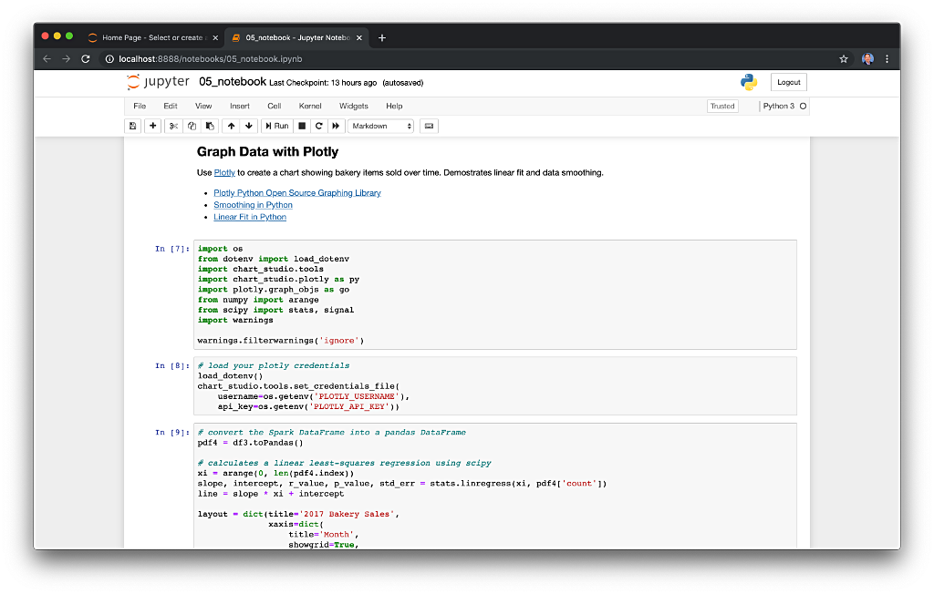
Shown below, we use Plotly to construct a bar chart of daily bakery items sold. The chart uses SciPy and NumPy to construct a linear fit (regression) and plot a line of best fit for the bakery data and overlaying the vertical bars. The chart also uses SciPy’s Savitzky-Golay Filter to plot the second line, illustrating a smoothing of our bakery data.
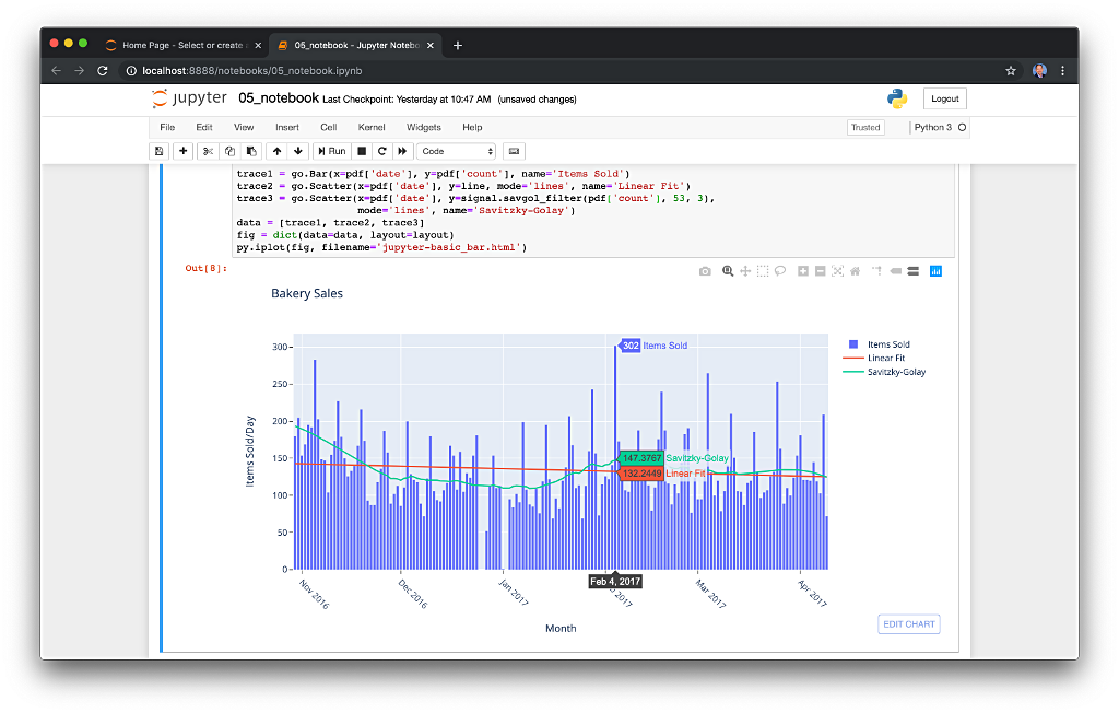
Plotly also provides Chart Studio Online Chart Maker. Plotly describes Chart Studio as the world’s most modern enterprise data visualization solutions. We can enhance, stylize, and share our data visualizations using the free version of Chart Studio Cloud.

Jupyter Notebook Viewer
Notebooks can also be viewed using nbviewer, an open-source project under Project Jupyter. Thanks to Rackspace hosting, the nbviewer instance is a free service.

Using nbviewer, below, we see the output of a cell within the 04_notebook.ipynb notebook. View this notebook, here, using nbviewer.

Monitoring Spark Jobs
The Jupyter Docker container exposes Spark’s monitoring and instrumentation web user interface. We can review each completed Spark Job in detail.

We can review details of each stage of the Spark job, including a visualization of the DAG (Directed Acyclic Graph), which Spark constructs as part of the job execution plan, using the DAG Scheduler.
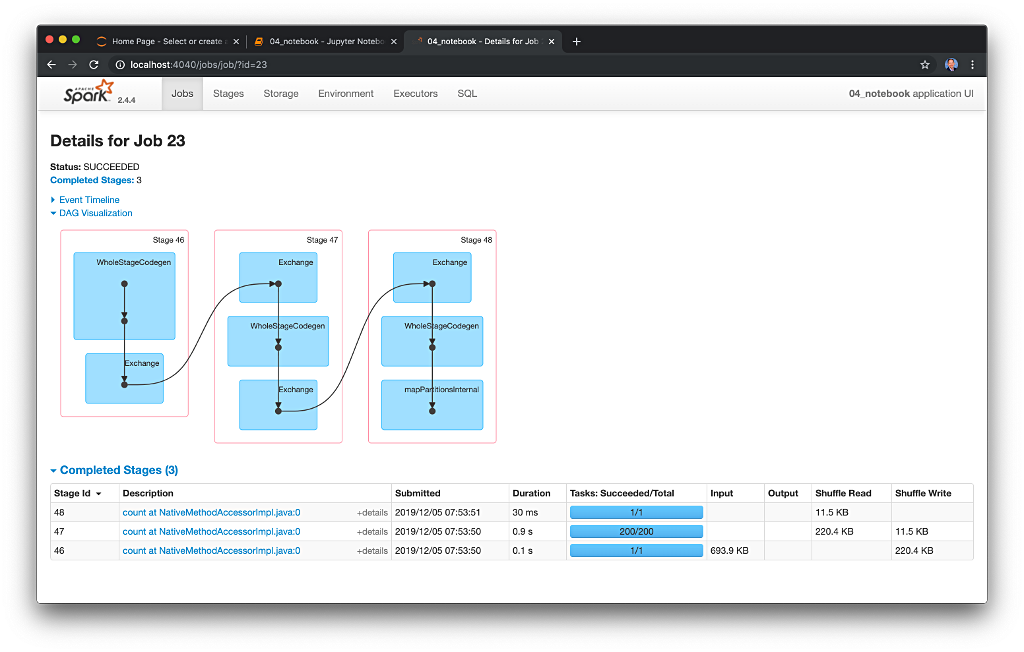
We can also review the task composition and timing of each event occurring as part of the stages of the Spark job.

We can also use the Spark interface to review and confirm the runtime environment configuration, including versions of Java, Scala, and Spark, as well as packages available on the Java classpath.

Local Spark Performance
Running Spark on a single node within the Jupyter Docker container on your local development system is not a substitute for a true Spark cluster, Production-grade, multi-node Spark clusters running on bare metal or robust virtualized hardware, and managed with Apache Hadoop YARN, Apache Mesos, or Kubernetes. In my opinion, you should only adjust your Docker resources limits to support an acceptable level of Spark performance for running small exploratory workloads. You will not realistically replace the need to process big data and execute jobs requiring complex calculations on a Production-grade, multi-node Spark cluster.

We can use the following docker stats command to examine the container’s CPU and memory metrics.
docker stats --format "table {{.Name}}\t{{.CPUPerc}}\t{{.MemUsage}}\t{{.MemPerc}}"
Below, we see the stats from the Docker stack’s three containers showing little or no activity.

Compare those stats with the ones shown below, recorded while a notebook was reading and writing data, and executing Spark SQL queries. The CPU and memory output show spikes, but both appear to be within acceptable ranges.

Linux Process Monitors
Another option to examine container performance metrics is top, which is pre-installed in our Jupyter container. For example, execute the following top command from a Jupyter terminal, sorting processes by CPU usage.
top -o %CPU
We should observe the individual performance of each process running in the Jupyter container.

A step up from top is htop, an interactive process viewer for Unix. It was installed in the container by the bootstrap script. For example, we can execute the htop command from a Jupyter terminal, sorting processes by CPU % usage.
htop --sort-key PERCENT_CPU
With htop, observe the individual CPU activity. Here, the four CPUs at the top left of the htop window are the CPUs assigned to Docker. We get insight into the way Spark is using multiple CPUs, as well as other performance metrics, such as memory and swap.

Assuming your development machine is robust, it is easy to allocate and deallocate additional compute resources to Docker if required. Be careful not to allocate excessive resources to Docker, starving your host machine of available compute resources for other applications.

Notebook Extensions
There are many ways to extend the Jupyter Docker Stacks. A popular option is jupyter-contrib-nbextensions. According to their website, the jupyter-contrib-nbextensions package contains a collection of community-contributed unofficial extensions that add functionality to the Jupyter notebook. These extensions are mostly written in JavaScript and will be loaded locally in your browser. Installed notebook extensions can be enabled, either by using built-in Jupyter commands, or more conveniently by using the jupyter_nbextensions_configurator server extension.
The project contains an alternate Docker stack file, stack-nbext.yml. The stack uses an alternative Docker image, garystafford/all-spark-notebook-nbext:latest, This Dockerfile, which builds it, uses the jupyter/all-spark-notebook:latest image as a base image. The alternate image adds in the jupyter-contrib-nbextensions and jupyter_nbextensions_configurator packages. Since Jupyter would need to be restarted after nbextensions is deployed, it cannot be done from within a running jupyter/all-spark-notebook container.
This file contains bidirectional Unicode text that may be interpreted or compiled differently than what appears below. To review, open the file in an editor that reveals hidden Unicode characters.
Learn more about bidirectional Unicode characters
| FROM jupyter/all-spark-notebook:latest | |
| USER root | |
| RUN pip install jupyter_contrib_nbextensions \ | |
| && jupyter contrib nbextension install –system \ | |
| && pip install jupyter_nbextensions_configurator \ | |
| && jupyter nbextensions_configurator enable –system \ | |
| && pip install yapf # for code pretty | |
| USER $NB_UID |
Using this alternate stack, below in our Jupyter container, we see the sizable list of extensions available. Some of my favorite extensions include ‘spellchecker’, ‘Codefolding’, ‘Code pretty’, ‘ExecutionTime’, ‘Table of Contents’, and ‘Toggle all line numbers’.

Below, we see five new extension icons that have been added to the menu bar of 04_notebook.ipynb. You can also observe the extensions have been applied to the notebook, including the table of contents, code-folding, execution time, and line numbering. The spellchecking and pretty code extensions were both also applied.

Conclusion
In this brief post, we have seen how easy it is to get started learning and performing data analytics using Jupyter notebooks, Python, Spark, and PySpark, all thanks to the Jupyter Docker Stacks. We could use this same stack to learn and perform machine learning using Scala and R. Extending the stack’s capabilities is as simple as swapping out this Jupyter image for another, with a different set of tools, as well as adding additional containers to the stack, such as MySQL, MongoDB, RabbitMQ, Apache Kafka, and Apache Cassandra.
All opinions expressed in this post are my own and not necessarily the views of my current or past employers, their clients.
Getting Started with Apache Zeppelin on Amazon EMR, using AWS Glue, RDS, and S3: Part 1
Posted by Gary A. Stafford in AWS, Bash Scripting, Big Data, Build Automation, Cloud, DevOps, Python, Software Development on November 22, 2019
Introduction
There is little question big data analytics, data science, artificial intelligence (AI), and machine learning (ML), a subcategory of AI, have all experienced a tremendous surge in popularity over the last 3–5 years. Behind the hype cycles and marketing buzz, these technologies are having a significant influence on many aspects of our modern lives. Due to their popularity, commercial enterprises, academic institutions, and the public sector have all rushed to develop hardware and software solutions to decrease the barrier to entry and increase the velocity of ML and Data Scientists and Engineers.
 Data Science: 5-Year Search Trend (courtesy Google Trends)
 Machine Learning: 5-Year Search Trend (courtesy Google Trends)
Technologies
All three major cloud providers, Amazon Web Services (AWS), Microsoft Azure, and Google Cloud, have rapidly maturing big data analytics, data science, and AI and ML services. AWS, for example, introduced Amazon Elastic MapReduce (EMR) in 2009, primarily as an Apache Hadoop-based big data processing service. Since then, according to Amazon, EMR has evolved into a service that uses Apache Spark, Apache Hadoop, and several other leading open-source frameworks to quickly and cost-effectively process and analyze vast amounts of data. More recently, in late 2017, Amazon released SageMaker, a service that provides the ability to build, train, and deploy machine learning models quickly and securely.
Simultaneously, organizations are building solutions that integrate and enhance these Cloud-based big data analytics, data science, AI, and ML services. One such example is Apache Zeppelin. Similar to the immensely popular Project Jupyter and the newly open-sourced Netflix’s Polynote, Apache Zeppelin is a web-based, polyglot, computational notebook. Zeppelin enables data-driven, interactive data analytics and document collaboration using a number of interpreters such as Scala (with Apache Spark), Python (with Apache Spark), Spark SQL, JDBC, Markdown, Shell and so on. Zeppelin is one of the core applications supported natively by Amazon EMR.

In the following two-part post, we will explore the use of Apache Zeppelin on EMR for data science and data analytics using a series of Zeppelin notebooks. The notebooks feature the use of AWS Glue, the fully managed extract, transform, and load (ETL) service that makes it easy to prepare and load data for analytics. The notebooks also feature the use of Amazon Relational Database Service (RDS) for PostgreSQL and Amazon Simple Cloud Storage Service (S3). Amazon S3 will serve as a Data Lake to store our unstructured data. Given the current choice of Zeppelin’s more than twenty different interpreters, we will use Python3 and Apache Spark, specifically Spark SQL and PySpark, for all notebooks.
We will build an economical single-node EMR cluster for data exploration, as well as a larger multi-node EMR cluster for analyzing large data sets. Amazon S3 will be used to store input and output data, while intermediate results are stored in the Hadoop Distributed File System (HDFS) on the EMR cluster. Amazon provides a good overview of EMR architecture. Below is a high-level architectural diagram of the infrastructure we will construct during Part 1 for this demonstration.
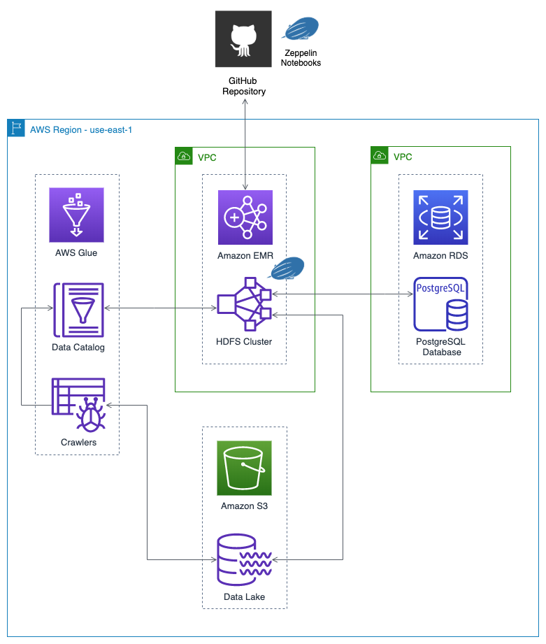
Notebook Features
Below is an overview of each Zeppelin notebook with a link to view it using Zepl’s free Notebook Explorer. Zepl was founded by the same engineers that developed Apache Zeppelin, including Moonsoo Lee, Zepl CTO and creator for Apache Zeppelin. Zepl’s enterprise collaboration platform, built on Apache Zeppelin, enables both Data Science and AI/ML teams to collaborate around data.
Notebook 1
The first notebook uses a small 21k row kaggle dataset, Transactions from a Bakery. The notebook demonstrates Zeppelin’s integration capabilities with the Helium plugin system for adding new chart types, the use of Amazon S3 for data storage and retrieval, and the use of Apache Parquet, a compressed and efficient columnar data storage format, and Zeppelin’s storage integration with GitHub for notebook version control.

Notebook 2
The second notebook demonstrates the use of a single-node and multi-node Amazon EMR cluster for the exploration and analysis of public datasets ranging from approximately 100k rows up to 27MM rows, using Zeppelin. We will use the latest GroupLens MovieLens rating datasets to examine the performance characteristics of Zeppelin, using Spark, on single- verses multi-node EMR clusters for analyzing big data using a variety of Amazon EC2 Instance Types.

Notebook 3
The third notebook demonstrates Amazon EMR and Zeppelin’s integration capabilities with AWS Glue Data Catalog as an Apache Hive-compatible metastore for Spark SQL. We will create an Amazon S3-based Data Lake using the AWS Glue Data Catalog and a set of AWS Glue Crawlers.
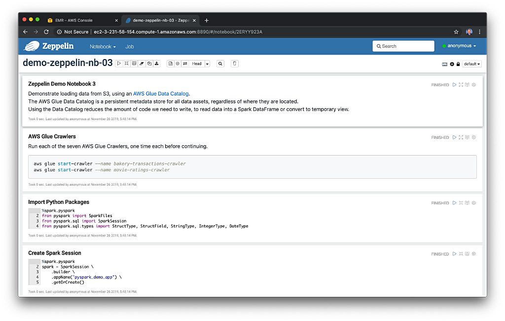
Notebook 4
The fourth notebook demonstrates Zeppelin’s ability to integrate with an external data source. In this case, we will interact with data in an Amazon RDS PostgreSQL relational database using three methods, including the Psycopg 2 PostgreSQL adapter for Python, Spark’s native JDBC capability, and Zeppelin’s JDBC Interpreter.

Demonstration
In Part 1 of the post, as a DataOps Engineer, we will create and configure the AWS resources required to demonstrate the use of Apache Zeppelin on EMR, using an AWS Glue Data Catalog, Amazon RDS PostgreSQL database, and an S3-based data lake. In Part 2 of this post, as a Data Scientist, we will explore Apache Zeppelin’s features and integration capabilities with a variety of AWS services using the Zeppelin notebooks.
Source Code
The demonstration’s source code is contained in two public GitHub repositories. The first repository, zeppelin-emr-demo, includes the four Zeppelin notebooks, organized according to the conventions of Zeppelin’s pluggable notebook storage mechanisms.
.
├── 2ERVVKTCG
│   └── note.json
├── 2ERYY923A
│   └── note.json
├── 2ESH8DGFS
│   └── note.json
├── 2EUZKQXX7
│   └── note.json
├── LICENSE
└── README.md
Zeppelin GitHub Storage
During the demonstration, changes made to your copy of the Zeppelin notebooks running on EMR will be automatically pushed back to GitHub when a commit occurs. To accomplish this, instead of just cloning a local copy of my zeppelin-emr-demo project repository, you will want your own copy, within your personal GitHub account. You could folk my zeppelin-emr-demo GitHub repository or copy a clone into your own GitHub repository.
To make a copy of the project in your own GitHub account, first, create a new empty repository on GitHub, for example, ‘my-zeppelin-emr-demo-copy’. Then, execute the following commands from your terminal, to clone the original project repository to your local environment, and finally, push it to your GitHub account.
# change me
GITHUB_ACCOUNT="your-account-name" # i.e. garystafford
GITHUB_REPO="your-new-project-name" # i.e. my-zeppelin-emr-demo-copy

# shallow clone into new directory
git clone --branch master \
    --single-branch --depth 1 --no-tags \
    https://github.com/garystafford/zeppelin-emr-demo.git \
    ${GITHUB_REPO}

# re-initialize repository
cd ${GITHUB_REPO}
rm -rf .git
git init

# re-commit code
git add -A
git commit -m "Initial commit of my copy of zeppelin-emr-demo"

# push to your repo
git remote add origin \
    https://github.com/$GITHUB_ACCOUNT/$GITHUB_REPO.git
git push -u origin master
GitHub Personal Access Token
To automatically push changes to your GitHub repository when a commit occurs, Zeppelin will need a GitHub personal access token. Create a personal access token with the scope shown below. Be sure to keep the token secret. Make sure you do not accidentally check your token value into your source code on GitHub. To minimize the risk, change or delete the token after completing the demo.

The second repository, zeppelin-emr-config, contains the necessary bootstrap files, CloudFormation templates, and PostgreSQL DDL (Data Definition Language) SQL script.
.
├── LICENSE
├── README.md
├── bootstrap
│   ├── bootstrap.sh
│   ├── emr-config.json
│   ├── helium.json
├── cloudformation
│   ├── crawler.yml
│   ├── emr_single_node.yml
│   ├── emr_cluster.yml
│   └── rds_postgres.yml
└── sql
    └── ratings.sql
Use the following AWS CLI command to clone the GitHub repository to your local environment.
git clone --branch master \
    --single-branch --depth 1 --no-tags \
    https://github.com/garystafford/zeppelin-emr-demo-setup.git
Requirements
To follow along with the demonstration, you will need an AWS Account, an existing Amazon S3 bucket to store EMR configuration and data, and an EC2 key pair. You will also need a current version of the AWS CLI installed in your work environment. Due to the particular EMR features, we will be using, I recommend using the us-east-1 AWS Region to create the demonstration’s resources.
# create secure emr config and data bucket
# change me
ZEPPELIN_DEMO_BUCKET="your-bucket-name"

aws s3api create-bucket \
    --bucket ${ZEPPELIN_DEMO_BUCKET}
aws s3api put-public-access-block \
    --bucket ${ZEPPELIN_DEMO_BUCKET} \
    --public-access-block-configuration \
    BlockPublicAcls=true,IgnorePublicAcls=true,BlockPublicPolicy=true,RestrictPublicBuckets=true
Copy Configuration Files to S3
To start, we need to copy three configuration files, bootstrap.sh, helium.json, and ratings.sql, from the zeppelin-emr-demo-setup project directory to our S3 bucket. Change the ZEPPELIN_DEMO_BUCKET variable value, then run the following s3 cp API command, using the AWS CLI. The three files will be copied to a bootstrap directory within your S3 bucket.
# change me
ZEPPELIN_DEMO_BUCKET="your-bucket-name"

aws s3 cp bootstrap/bootstrap.sh s3://${ZEPPELIN_DEMO_BUCKET}/bootstrap/
aws s3 cp bootstrap/helium.json s3://${ZEPPELIN_DEMO_BUCKET}/bootstrap/
aws s3 cp sql/ratings.sql s3://${ZEPPELIN_DEMO_BUCKET}/bootstrap/
Below, sample output from copying local files to S3.

Create AWS Resources
We will start by creating most of the required AWS resources for the demonstration using three CloudFormation templates. We will create a single-node Amazon EMR cluster, an Amazon RDS PostgresSQL database, an AWS Glue Data Catalog database, two AWS Glue Crawlers, and a Glue IAM Role. We will wait to create the multi-node EMR cluster due to the compute costs of running large EC2 instances in the cluster. You should understand the cost of these resources before proceeding, and that you ensure they are destroyed immediately upon completion of the demonstration to minimize your expenses.
Single-Node EMR Cluster
We will start by creating the single-node Amazon EMR cluster, consisting of just one master node with no core or task nodes (a cluster of one). All operations will take place on the master node.
Default EMR Resources
The following EMR instructions assume you have already created at least one EMR cluster in the past, in your current AWS Region, using the EMR web interface with the ‘Create Cluster – Quick Options’ option. Creating a cluster this way creates several additional AWS resources, such as the EMR_EC2_DefaultRole EC2 instance profile, the default EMR_DefaultRole EMR IAM Role, and the default EMR S3 log bucket.

If you haven’t created any EMR clusters using the EMR ‘Create Cluster – Quick Options’ in the past, don’t worry, you can also create the required resources with a few quick AWS CLI commands. Change the following LOG_BUCKET variable value, then run the aws emr and aws s3api API commands, using the AWS CLI. The LOG_BUCKET variable value follows the convention of aws-logs-awsaccount-region. For example, aws-logs-012345678901-us-east-1.
# create emr roles
aws emr create-default-roles

# create log secure bucket
# change me
LOG_BUCKET="aws-logs-your_aws_account_id-your_region"

aws s3api create-bucket --bucket ${LOG_BUCKET}
aws s3api put-public-access-block --bucket ${LOG_BUCKET} \
    --public-access-block-configuration \
    BlockPublicAcls=true,IgnorePublicAcls=true,BlockPublicPolicy=true,RestrictPublicBuckets=true
The new EMR IAM Roles can be viewed in the IAM Roles web interface.

Often, I see tutorials that reference these default EMR resources from the AWS CLI or CloudFormation, without any understanding or explanation of how they are created.
EMR Bootstrap Script
As part of creating our EMR cluster, the CloudFormation template, emr_single_node.yml, will call the bootstrap script we copied to S3, earlier, bootstrap.sh. The bootstrap script pre-installs required Python and Linux software packages, and the PostgreSQL driver JAR. The bootstrap script also clones your copy of the zeppelin-emr-demo GitHub repository.
#!/bin/bash
set -ex

if [[ $# -ne 2 ]] ; then
    echo "Script requires two arguments"
    exit 1
fi

GITHUB_ACCOUNT=$1
GITHUB_REPO=$2

# install extra python packages
sudo python3 -m pip install psycopg2-binary boto3

# install extra linux packages
yes | sudo yum install git htop

# clone github repo
cd /tmp
git clone "https://github.com/${GITHUB_ACCOUNT}/${GITHUB_REPO}.git"

# install extra jars
POSTGRES_JAR="postgresql-42.2.8.jar"
wget -nv "https://jdbc.postgresql.org/download/${POSTGRES_JAR}"
sudo chown -R hadoop:hadoop ${POSTGRES_JAR}
mkdir -p /home/hadoop/extrajars/
cp ${POSTGRES_JAR} /home/hadoop/extrajars/
EMR Application Configuration
The EMR CloudFormation template will also modify the EMR cluster’s Spark and Zeppelin application configurations. Amongst other configuration properties, the template sets the default Python version to Python3, instructs Zeppelin to use the cloned GitHub notebook directory path, and adds the PostgreSQL Driver JAR to the JVM ClassPath. Below we can see the configuration properties applied to an existing EMR cluster.

EMR Application Versions
As of the date of this post, EMR is at version 5.28.0. Below, as shown in the EMR web interface, are the current (21) applications and frameworks available for installation on EMR.

For this demo, we will install Apache Spark v2.4.4, Ganglia v3.7.2, and Zeppelin 0.8.2.
 Apache Zeppelin: Web Interface
 Apache Spark: DAG Visualization
 Ganglia: Cluster CPU Monitoring
Create the EMR CloudFormation Stack
Change the following (7) variable values, then run the emr cloudformation create-stack API command, using the AWS CLI.
# change me
ZEPPELIN_DEMO_BUCKET="your-bucket-name"
EC2_KEY_NAME="your-key-name"
LOG_BUCKET="aws-logs-your_aws_account_id-your_region"
GITHUB_ACCOUNT="your-account-name" # i.e. garystafford
GITHUB_REPO="your-new-project-name" # i.e. my-zeppelin-emr-demo
GITHUB_TOKEN="your-token-value"
MASTER_INSTANCE_TYPE="m5.xlarge" # optional

aws cloudformation create-stack \
    --stack-name zeppelin-emr-dev-stack \
    --template-body file://cloudformation/emr_single_node.yml \
    --parameters ParameterKey=ZeppelinDemoBucket,ParameterValue=${ZEPPELIN_DEMO_BUCKET} \
                 ParameterKey=Ec2KeyName,ParameterValue=${EC2_KEY_NAME} \
                 ParameterKey=LogBucket,ParameterValue=${LOG_BUCKET} \
                 ParameterKey=MasterInstanceType,ParameterValue=${MASTER_INSTANCE_TYPE} \
                 ParameterKey=GitHubAccount,ParameterValue=${GITHUB_ACCOUNT} \
                 ParameterKey=GitHubRepository,ParameterValue=${GITHUB_REPO} \
                 ParameterKey=GitHubToken,ParameterValue=${GITHUB_TOKEN}
You can use the Amazon EMR web interface to confirm the results of the CloudFormation stack. The cluster should be in the ‘Waiting’ state.

PostgreSQL on Amazon RDS
Next, create a simple, single-AZ, single-master, non-replicated Amazon RDS PostgreSQL database, using the included CloudFormation template, rds_postgres.yml. We will use this database in Notebook 4. For the demo, I have selected the current-generation general purpose db.m4.large EC2 instance type to run PostgreSQL. You can easily change the instance type to another RDS-supported instance type to suit your own needs.
Change the following (3) variable values, then run the cloudformation create-stack API command, using the AWS CLI.
# change me
DB_MASTER_USER="your-db-username" # i.e. masteruser
DB_MASTER_PASSWORD="your-db-password" # i.e. 5up3r53cr3tPa55w0rd
MASTER_INSTANCE_TYPE="db.m4.large" # optional

aws cloudformation create-stack \
    --stack-name zeppelin-rds-stack \
    --template-body file://cloudformation/rds_postgres.yml \
    --parameters ParameterKey=DBUser,ParameterValue=${DB_MASTER_USER} \
                 ParameterKey=DBPassword,ParameterValue=${DB_MASTER_PASSWORD} \
                 ParameterKey=DBInstanceClass,ParameterValue=${MASTER_INSTANCE_TYPE}
You can use the Amazon RDS web interface to confirm the results of the CloudFormation stack.

AWS Glue
Next, create the AWS Glue Data Catalog database, the Apache Hive-compatible metastore for Spark SQL, two AWS Glue Crawlers, and a Glue IAM Role (ZeppelinDemoCrawlerRole), using the included CloudFormation template, crawler.yml. The AWS Glue Data Catalog database will be used in Notebook 3.
Change the following variable value, then run the cloudformation create-stack API command, using the AWS CLI.
# change me
ZEPPELIN_DEMO_BUCKET="your-bucket-name"

aws cloudformation create-stack \
    --stack-name zeppelin-crawlers-stack \
    --template-body file://cloudformation/crawler.yml \
    --parameters ParameterKey=ZeppelinDemoBucket,ParameterValue=${ZEPPELIN_DEMO_BUCKET} \
    --capabilities CAPABILITY_NAMED_IAM
You can use the AWS Glue web interface to confirm the results of the CloudFormation stack. Note the Data Catalog database and the two Glue Crawlers. We will not run the two crawlers until Part 2 of the post, so no tables will exist in the Data Catalog database, yet.


At this point in the demonstration, you should have successfully created a single-node Amazon EMR cluster, an Amazon RDS PostgresSQL database, and several AWS Glue resources, all using CloudFormation templates.

Post-EMR Creation Configuration
RDS Security
For the new EMR cluster to communicate with the RDS PostgreSQL database, we need to ensure that port 5432 is open from the RDS database’s VPC security group, which is the default VPC security group, to the security groups of the EMR nodes. Obtain the Group ID of the ElasticMapReduce-master and ElasticMapReduce-slave Security Groups from the EMR web interface.

Access the Security Group for the RDS database using the RDS web interface. Change the inbound rule for port 5432 to include both Security Group IDs.

SSH to EMR Master Node
In addition to the bootstrap script and configurations, we already applied to the EMR cluster, we need to make several post-EMR creation configuration changes to the EMR cluster for our demonstration. These changes will require SSH’ing to the EMR cluster. Using the master node’s public DNS address and SSH command provided in the EMR web console, SSH into the master node.

If you cannot access the node using SSH, check that port 22 is open on the associated EMR master node IAM Security Group (ElasticMapReduce-master) to your IP address or address range.


Git Permissions
We need to change permissions on the git repository we installed during the EMR bootstrapping phase. Typically, with an EC2 instance, you perform operations as the ec2-user user. With Amazon EMR, you often perform actions as the hadoop user. With Zeppelin on EMR, the notebooks perform operations, including interacting with the git repository as the zeppelin user. As a result of the bootstrap.sh script, the contents of the git repository directory, /tmp/zeppelin-emr-demo/, are owned by the hadoop user and group by default.

We will change their owner to the zeppelin user and group. We could not perform this step as part of the bootstrap script since the the zeppelin user and group did not exist at the time the script was executed.
cd /tmp/zeppelin-emr-demo/
sudo chown -R zeppelin:zeppelin .
The results should look similar to the following output.

Pre-Install Visualization Packages
Next, we will pre-install several Apache Zeppelin Visualization packages. According to the Zeppelin website, an Apache Zeppelin Visualization is a pluggable package that can be loaded/unloaded on runtime through the Helium framework in Zeppelin. We can use them just like any other built-in visualization in the notebook. A Visualization is a javascript npm package. For example, here is a link to the ultimate-pie-chart on the public npm registry.
We can pre-load plugins by replacing the /usr/lib/zeppelin/conf/helium.json file with the version of helium.json we copied to S3, earlier, and restarting Zeppelin. If you have a lot of Visualizations or package types or use any DataOps automation to create EMR clusters, this approach is much more efficient and repeatable than manually loading plugins using the Zeppelin UI, each time you create a new EMR cluster. Below, the helium.json file, which pre-loads (8) Visualization packages.
{
    "enabled": {
        "ultimate-pie-chart": "ultimate-pie-chart@0.0.2",
        "ultimate-column-chart": "ultimate-column-chart@0.0.2",
        "ultimate-scatter-chart": "ultimate-scatter-chart@0.0.2",
        "ultimate-range-chart": "ultimate-range-chart@0.0.2",
        "ultimate-area-chart": "ultimate-area-chart@0.0.1",
        "ultimate-line-chart": "ultimate-line-chart@0.0.1",
        "zeppelin-bubblechart": "zeppelin-bubblechart@0.0.4",
        "zeppelin-highcharts-scatterplot": "zeppelin-highcharts-scatterplot@0.0.2"
    },
    "packageConfig": {},
    "bundleDisplayOrder": [
        "ultimate-pie-chart",
        "ultimate-column-chart",
        "ultimate-scatter-chart",
        "ultimate-range-chart",
        "ultimate-area-chart",
        "ultimate-line-chart",
        "zeppelin-bubblechart",
        "zeppelin-highcharts-scatterplot"
    ]
}
Run the following commands to load the plugins and adjust the permissions on the file.
# change me
ZEPPELIN_DEMO_BUCKET="your-bucket-name"

sudo aws s3 cp s3://${ZEPPELIN_DEMO_BUCKET}/bootstrap/helium.json \
    /usr/lib/zeppelin/conf/helium.json
sudo chown zeppelin:zeppelin /usr/lib/zeppelin/conf/helium.json
Create New JDBC Interpreter
Lastly, we need to create a new Zeppelin JDBC Interpreter to connect to our RDS database. By default, Zeppelin has several interpreters installed. You can review a list of available interpreters using the following command.
sudo sh /usr/lib/zeppelin/bin/install-interpreter.sh --list

The new JDBC interpreter will allow us to connect to our RDS PostgreSQL database, using Java Database Connectivity (JDBC). First, ensure all available interpreters are installed, including the current Zeppelin JDBC driver (org.apache.zeppelin:zeppelin-jdbc:0.8.0) to /usr/lib/zeppelin/interpreter/jdbc.
Creating a new interpreter is a two-part process. In this stage, we install the required interpreter files on the master node using the following command. Then later, in the Zeppelin web interface, we will configure the new PostgreSQL JDBC interpreter. Note we must provide a unique name for the interpreter (I chose ‘postgres’ in this case), which we will refer to in part two of the interpreter creation process.
sudo sh /usr/lib/zeppelin/bin/install-interpreter.sh --all

sudo sh /usr/lib/zeppelin/bin/install-interpreter.sh \
    --name "postgres" \
    --artifact org.apache.zeppelin:zeppelin-jdbc:0.8.0
To complete the post-EMR creation configuration on the master node, we must restart Zeppelin for our changes to take effect.
sudo stop zeppelin && sudo start zeppelin
In my experience, it could take 2–3 minutes for the Zeppelin UI to become fully responsive after a restart.

Zeppelin Web Interface Access
With all the EMR application configuration complete, we will access the Zeppelin web interface running on the master node. Use the Zeppelin connection information provided in the EMR web interface to setup SSH tunneling to the Zeppelin web interface, running on the master node. Using this method, we can also access the Spark History Server, Ganglia, and Hadoop Resource Manager web interfaces; all links are provided from EMR.

To set up a web connection to the applications installed on the EMR cluster, I am using FoxyProxy as a proxy management tool with Google Chrome.

If everything is working so far, you should see the Zeppelin web interface with all four Zeppelin notebooks available from the cloned GitHub repository. You will be logged in as the anonymous user. Zeppelin offers authentication for accessing notebooks on the EMR cluster. For brevity, we will not cover setting up authentication in Zeppelin, using Shiro Authentication.
To confirm the path to the local, cloned copy of the GitHub notebook repository, is correct, check the Notebook Repos interface, accessible under the Settings dropdown (anonymous user) in the upper right of the screen. The value should match the ZEPPELIN_NOTEBOOK_DIR configuration property value in the emr_single_node.yml CloudFormation template we executed earlier.

To confirm the Helium Visualizations were pre-installed correctly, using the helium.json file, open the Helium interface, accessible under the Settings dropdown (anonymous user) in the upper right of the screen.
 Note the enabled visualizations. And, it is easy to enable additional plugins through the web interface.
New PostgreSQL JDBC Interpreter
If you recall, earlier, we install the required interpreter files on the master node using the following command using the bootstrap script. We will now complete the process of configuring the new PostgreSQL JDBC interpreter. Open the Interpreter interface, accessible under the Settings dropdown (anonymous user) in the upper right of the screen.
The title of the new interpreter must match the name we used to install the interpreter files, ‘postgres’. The interpreter group will be ‘jdbc’. There are, minimally, three properties we need to configure for your specific RDS database instance, including default.url, default.user, and default.password. These should match the values you used to create your RDS instance, earlier. Make sure to includes the database name in the default.url. An example is shown below.
default.url: jdbc:postgresql://zeppelin-demo.abcd1234efg56.us-east-1.rds.amazonaws.com:5432/ratings
default.user: masteruser
default.password: 5up3r53cr3tPa55w0rd
We also need to provide a path to the PostgreSQL driver JAR dependency. This path is the location where we placed the JAR using the bootstrap.sh script, earlier, /home/hadoop/extrajars/postgresql-42.2.8.jar. Save the new interpreter and make sure it starts successfully (shows a green icon).


Switch Interpreters to Python 3
The last thing we need to do is change the Spark and Python interpreters to use Python 3 instead of the default Python 2. On the same screen you used to create a new interpreter, modify the Spark and Python interpreters. First, for the Python interpreter, change the zeppelin.python property to python3.

Next, for the Spark interpreter, change the zeppelin.pyspark.python property to python3.

Part 2
In Part 1 of this post, we created and configured the AWS resources required to demonstrate the use of Apache Zeppelin on EMR, using an AWS Glue Data Catalog, Amazon RDS PostgreSQL database, and an S3 data lake. In Part 2 of this post, we will explore some of Apache Zeppelin’s features and integration capabilities with a variety of AWS services using the notebooks.
All opinions expressed in this post are my own and not necessarily the views of my current or past employers or their clients.
Gary Stafford
AWS Area Principal Solutions Architect | 10x AWS Certified Pro | DevOps | Data/ML | Serverless | Polyglot Developer | Former ThoughtWorks and Accenture
