Posts Tagged Streaming data

Streaming Data on AWS: Amazon Kinesis Data Streams or Amazon MSK?

Posted by Gary A. Stafford in Analytics, AWS, Big Data, Serverless on April 23, 2023

Given similar functionality, what differences make one AWS-managed streaming service a better choice over the other?

Kinesis Data Streams and Amazon MSK can often be used interchangeably in streaming data workflows

Data streaming has emerged as a powerful tool in the last few years thanks to its ability to quickly and efficiently process large volumes of data, provide real-time insights, and scale and adapt to meet changing needs. As IoT, social media, and mobile devices continue to generate vast amounts of data, it has become imperative to have platforms that can handle the real-time ingestion, processing, and analysis of this data.

Key Differentiators

Amazon Kinesis Data Streams and Amazon Managed Streaming for Apache Kafka (Amazon MSK) are two managed streaming services offered by AWS. While both platforms offer similar features, choosing the right service largely depends on your specific use cases and business requirements.

Amazon Kinesis Data Streams

Simplicity: Kinesis Data Streams is generally considered a less complicated service than Amazon MSK, which requires you to manage more of the underlying infrastructure. This can make setting up and managing your streaming data pipeline easier, especially if you have limited experience with Apache Kafka. Amazon MSK Serverless, which went GA in April 2022, is a cluster type for Amazon MSK that allows you to run Apache Kafka without managing and scaling cluster capacity. Unlike Amazon MSK provisioned, Amazon MSK Serverless greatly reduces the effort required to use Amazon MSK, making ‘Simplicity’ less of a Kinesis differentiator.
Integration with AWS services: Kinesis Data Streams integrates well with other AWS services, such as AWS Lambda, Amazon S3, and Amazon OpenSearch. This can make building end-to-end data processing pipelines easier using these services.
Low latency: Kinesis Data Streams is designed to deliver low-latency processing of streaming data, which can be important for applications that require near real-time processing.
Predictable pricing: Kinesis Data Streams is generally considered to have a more predictable pricing model than Amazon MSK, based on instance sizes and hourly usage. With Kinesis Data Streams, you pay for the data you process, making estimating and managing fees easier (additional fees may apply).

Example Architecture #1: Ingestion of features into SageMaker Feature Store using Amazon Kinesis

Amazon MSK

Compatibility with Apache Kafka: Amazon MSK may be a better choice if you have an existing Apache Kafka deployment or are already familiar with Kafka. Amazon MSK is a fully managed version of Apache Kafka, which you can use with existing Kafka applications and tools.
Customization: With Amazon MSK, you have more control over the underlying cluster infrastructure, configuration, deployment, and version of Kafka, which means you can customize the cluster to meet your needs. This can be important if you have specialized requirements or want to optimize performance (e.g., high-volume financial trading, real-time gaming).
Larger ecosystem: Apache Kafka has a large ecosystem of tools and integrations compared to Kinesis Data Streams. This can provide flexibility and choice when building and managing your streaming data pipeline. Some common tools include MirrorMaker, Kafka Connect, LinkedIn’s Cruise Control, kcat (fka kafkacat), Lenses, Confluent Schema Registry, and Appicurio Registry.
Preference for Open Source: You may prefer the flexibility, transparency, pace of innovation, and interoperability of employing open source software (OSS) over proprietary software and services for your streaming solution.

Ultimately, the choice between Amazon Kinesis Data Streams and Amazon MSK will depend on your specific needs and priorities. Kinesis Data Streams might be better if you prioritize simplicity, integration with other AWS services, and low latency. If you have an existing Kafka deployment, require more customization, or need access to a larger ecosystem of tools and integrations, Amazon MSK might be a better fit. In my opinion, the newer Amazon MSK Serverless option lessens several traditional differentiators between the two services.

Scaling Capabilities

Amazon Kinesis Data Streams and Amazon MSK are designed to be scalable streaming services that can handle large volumes of data. However, there are some differences in their scaling capabilities.

Amazon Kinesis Data Streams

Scalability: Kinesis Data Streams has two capacity modes, on-demand and provisioned. With the on-demand mode, Kinesis Data Streams automatically manages the shards to provide the necessary throughput based on the amount of data you process. This means the service can automatically adjust the number of shards based on the incoming data volume, allowing you to handle increased traffic without manually adjusting the infrastructure.
Limitations: Per the documentation, there is no upper quota on the number of streams with the provisioned mode you can have in an account. A shard can ingest up to 1 MB of data per second (including partition keys) or 1,000 records per second for writes. The maximum size of the data payload of a record before base64-encoding is up to 1 MB. GetRecords can retrieve up to 10 MB of data per call from a single shard and up to 10,000 records per call. Each call to GetRecords is counted as one read transaction. Each shard can support up to five read transactions per second. Each read transaction can provide up to 10,000 records with an upper quota of 10 MB per transaction. Each shard can support a maximum total data read rate of 2 MB per second via GetRecords. If a call to GetRecords returns 10 MB, subsequent calls made within the next 5 seconds throw an exception.
Cost: Kinesis Data Streams has two capacity modes — on-demand and provisioned — with different pricing models. With on-demand capacity mode, you pay per GB of data written and read from your data streams. You do not need to specify how much read and write throughput you expect your application to perform. With provisioned capacity mode, you select the number of shards necessary for your application based on its write and read request rate. There are additional fees PUT Payload Units, enhanced fan-out, extended data retention, and retrieval of long-term retention data.

Amazon MSK

Scalability: Amazon MSK is designed to be highly scalable and can handle millions of messages per second. With Amazon MSK provisioned, you can scale your Kafka cluster by adding or removing instances (brokers) and storage as needed. Amazon MSK can automatically rebalance partitions across instances. Alternately, Amazon MSK Serverless automatically provisions and scales capacity while managing the partitions in your topic, so you can stream data without thinking about right-sizing or scaling clusters.
Flexibility: With Amazon MSK, you have more control over the underlying infrastructure, which means you can customize the deployment to meet your needs. This can be important if you have specialized requirements or want to optimize performance.
Amazon MSK also offers multiple authentication methods. You can use IAM to authenticate clients and to allow or deny Apache Kafka actions. Alternatively, with Amazon MSK provisioned, you can use TLS or SASL/SCRAM to authenticate clients and Apache Kafka ACLs to allow or deny actions.
Cost: Scaling up or down with Amazon MSK can impact the cost based on instance sizes and hourly usage. Therefore, adding more instances can increase the overall cost of the service. Pricing models for Amazon MSK and Amazon MSK Serverless vary.

Amazon Kinesis Data Streams and Amazon MSK are highly scalable services. Kinesis Data Streams can scale automatically based on the amount of data you process. At the same time, Amazon MSK allows you to scale your Kafka cluster by adding or removing instances and adding storage as needed. However, adding more shards with Kinesis can lead to a more manual process that can take some time to propagate and impact cost, while scaling up or down with Amazon MSK is based on instance sizes and hourly usage. Ultimately, the choice between the two will depend on your specific use case and requirements.

Throughput

Throughput can be measured in the maximum MB/s of data and the maximum number of records per second. The maximum throughput of both Amazon Kinesis Data Streams and Amazon MSK are not hard limits. Depending on the service, you can exceed these limits by adding more resources, including shards or brokers. Total maximum system throughput is affected by the maximum throughput of both upstream and downstream producing and consuming components.

Amazon Kinesis Data Streams

The maximum throughput of Kinesis Data Streams depends on the number of shards and the size of the data being processed. Each shard in a Kinesis stream can handle up to 1 MB/s of data input and up to 2 MB/s of data output, or up to 1,000 records per second for writes and up to 10,000 records per second for reads. When a consumer uses enhanced fan-out, it gets its own 2 MB/s allotment of read throughput, allowing multiple consumers to read data from the same stream in parallel without contending for read throughput with other consumers.

The maximum throughput of a Kinesis stream is determined by the number of shards you have multiplied by the maximum throughput per shard. For example, if you have a stream with 10 shards, the maximum throughput of the stream would be 10 MB/s for data input and 20 MB/s for data output, or up to 10,000 records per second for writes and up to 100,000 records per second for reads.

The maximum throughput is not a hard limit, and you can exceed these limits by adding more shards to your stream. However, adding more shards can impact the cost of the service, and you should consider the optimal shard count for your use case to ensure efficient and cost-effective processing of your data.

Amazon MSK

As discussed in the Amazon MSK best practices documentation, the maximum throughput of Amazon MSK depends on the number of brokers and the instance type of those brokers. Amazon MSK allows you to scale the number of instances in a Kafka cluster up or down based on your needs.

The maximum throughput of an Amazon MSK cluster depends on the number of brokers and the performance characteristics of the instance types you are using. Each broker in an Amazon MSK cluster can handle tens of thousands of messages per second, depending on the instance type and configuration. The actual throughput you can achieve will depend on your specific use case and the message size. The AWS blog post, Best practices for right-sizing your Apache Kafka clusters to optimize performance and cost, is an excellent reference.

The maximum throughput is not a hard limit, and you can exceed these limits by adding more brokers or upgrading to more powerful instances. However, adding more instances or upgrading to more powerful instances can impact the service’s cost. Therefore, consider your use case’s optimal instance count and type to ensure efficient and cost-effective data processing.

Writing Messages

Compatibility with multiple producers and consumers is essential when choosing a streaming technology. There are multiple ways to write messages to Amazon Kinesis Data Streams and Amazon MSK.

Amazon Kinesis Data Streams

AWS SDK: Use the AWS SDK for your preferred programming language.
Kinesis Producer Library (KPL): KPL is a high-performance library that allows you to write data to Kinesis Data Streams at a high rate. KPL handles all heavy lifting, including batching, retrying failed records, and load balancing across shards.
Amazon Kinesis Data Firehose: Kinesis Data Firehose is a fully managed service that can ingest and transform streaming data in real-time. It can be used to write data to Kinesis Data Streams, as well as to other AWS services such as S3, Redshift, and Elasticsearch.
Amazon Kinesis Data Analytics: Kinesis Data Analytics is a fully managed service that allows you to process and analyze streaming data in real-time. It can read data from Kinesis Data Streams, perform real-time analytics and transformations, and write the results to another Kinesis stream or an external data store.
Kinesis Agent: Kinesis Agent is a standalone Java application that collects and sends data to Kinesis Data Streams. It can monitor log files or other data sources and automatically send data to Kinesis Data Streams as it is generated.
Third-party libraries and tools: There are many third-party libraries and tools available for writing data to Kinesis Data Streams, including Apache Kafka Connect, Apache Storm, and Fluentd. These tools can integrate Kinesis Data Streams with existing data processing pipelines or build custom streaming applications.

Example Architecture #3: Example of using Kinesis Producer Library to write messages to Kinesis Data Streams

Amazon MSK

Kafka command line tools: The Kafka command line tools (e.g., kafka-console-producer.sh) can be used to write messages to a Kafka topic in an Amazon MSK cluster. These tools are part of the Kafka distribution and are pre-installed on the Amazon MSK broker nodes.
Kafka client libraries: You can use Kafka client libraries in your preferred programming language (e.g., Java, Python, C#) to write messages to an Amazon MSK cluster. These libraries provide a more flexible and customizable way to produce messages to Kafka topics.
AWS SDKs: You can use AWS SDKs (e.g., AWS SDK for Java, AWS SDK for Python) to interact with Amazon MSK and write messages to Kafka topics. These SDKs provide a higher-level abstraction over the Kafka client libraries, making integrating Amazon MSK into your AWS infrastructure easier.
Third-party libraries and tools: There are many third-party tools and frameworks, including Apache NiFi, Apache Camel, and Apache Beam. They provide Kafka connectors and producers, which can be used to write messages to Kafka topics in Amazon MSK. These tools can simplify the process of writing messages and provide additional features such as data transformation and routing.

Schema Registry

You can use AWS Glue Schema Registry with Amazon Kinesis Data Streams and Amazon MSK. AWS Glue Schema Registry is a fully managed service that provides a central schema repository for organizing, validating, and tracking the evolution of your data schemas. It enables you to store, manage, and discover schemas for your data in a single, centralized location.

With AWS Glue Schema Registry, you can define and register schemas for your data in the registry. You can then use these schemas to validate the data being ingested into your streaming applications, ensuring that the data conforms to the expected structure and format.

Both Kinesis Data Streams and Amazon MSK support the use of AWS Glue Schema Registry through the use of Apache Avro schemas. Avro is a compact, fast, binary data format that can improve the performance of your streaming applications. You can configure your streaming applications to use the registry to validate incoming data, ensuring that it conforms to the schema before processing.

Using AWS Glue Schema Registry can help ensure the consistency and quality of your data across your streaming applications and provide a centralized location for managing and tracking schema changes. Amazon MSK is also compatible with popular alternative schema registries, such as Confluent Schema Registry and RedHat’s open-source Apicurio Registry.

Example Architecture #4: Change Data Capture (CDC) using Amazon MSK and Glue Schema Registry

Stream Processing

According to TechTarget, Stream processing is a data management technique that involves ingesting a continuous data stream to quickly analyze, filter, transform, or enhance the data in real-time. Several leading stream processing tools are available, compatible with Amazon Kinesis Data Streams and Amazon MSK. Each tool with its own strengths and use cases. Some of the more popular tools include:

Apache Flink: Apache Flink is a distributed stream processing framework that provides fast, scalable, and fault-tolerant data processing for real-time and batch data streams. It supports a variety of data sources and sinks and provides a powerful stream processing API and SQL interface. In addition, Amazon offers its managed version of Apache Flink, Amazon Kinesis Data Analytics (KDA), which is compatible with both Amazon Kinesis Data Streams and Amazon MSK.
Apache Spark Structured Streaming: Apache Spark Structured Streaming is a stream processing framework that allows developers to build real-time stream processing applications using the familiar Spark API. It provides high-level APIs for processing data streams and supports integration with various data sources and sinks. Apache Spark is compatible with both Amazon Kinesis Data Streams and Amazon MSK. Spark Streaming is available as a managed service on AWS via AWS Glue Studio and Amazon EMR.
Apache NiFi: Apache NiFi is an open-source data integration and processing tool that provides a web-based UI for building data pipelines. It supports batch and stream processing and offers a variety of processors for data ingestion, transformation, and delivery. Apache NiFi is compatible with both Amazon Kinesis Data Streams and Amazon MSK.
Amazon Kinesis Data Firehose (KDA): Kinesis Data Firehose is a fully managed service that can ingest and transform streaming data in real time. It can be used to write data to Kinesis Data Streams, as well as to other AWS services such as S3, Redshift, and Elasticsearch. Kinesis Data Firehose is compatible with Amazon Kinesis Data Streams and Amazon MSK.
Apache Kafka Streams (aka KStream): Apache Kafka Streams is a lightweight stream processing library that allows developers to build scalable and fault-tolerant real-time applications and microservices. KStreams integrates seamlessly with Amazon MSK and provides a high-level DSL for stream processing.
ksqlDB: ksqlDB is a database for building stream processing applications on top of Apache Kafka. It is distributed, scalable, reliable, and real-time. ksqlDB combines the power of real-time stream processing with the approachable feel of a relational database through a familiar, lightweight SQL syntax. ksqlDB is compatible with Amazon MSK.

Several stream-processing tools are detailed in my recent two-part blog post, Exploring Popular Open-source Stream Processing Technologies.

Conclusion

Amazon Kinesis Data Streams and Amazon Managed Streaming for Apache Kafka (Amazon MSK) are managed streaming services. While they offer similar functionality, some differences might make one a better choice, depending on your use cases and experience. Ensure you understand your streaming requirements and each service’s capabilities before making a final architectural decision.

🔔 To keep up with future content, follow Gary Stafford on LinkedIn.

This blog represents my viewpoints and not those of my employer, Amazon Web Services (AWS). All product names, logos, and brands are the property of their respective owners.

Amazon Kinesis Data Streams, Amazon Managed Streaming for Apache Kafka, Amazon MSK, Amazon Web Services, AWS, Stream Processing, Streaming data

Exploring Popular Open-source Stream Processing Technologies: Part 2 of 2

Posted by Gary A. Stafford in Analytics, Big Data, Java Development, Python, Software Development, SQL on September 26, 2022

A brief demonstration of Apache Spark Structured Streaming, Apache Kafka Streams, Apache Flink, and Apache Pinot with Apache Superset

Introduction

According to TechTarget, “Stream processing is a data management technique that involves ingesting a continuous data stream to quickly analyze, filter, transform or enhance the data in real-time. Once processed, the data is passed off to an application, data store, or another stream processing engine.” Confluent, a fully-managed Apache Kafka market leader, defines stream processing as “a software paradigm that ingests, processes, and manages continuous streams of data while they’re still in motion.”

This two-part post series and forthcoming video explore four popular open-source software (OSS) stream processing projects: Apache Spark Structured Streaming, Apache Kafka Streams, Apache Flink, and Apache Pinot.

This post uses the open-source projects, making it easier to follow along with the demonstration and keeping costs to a minimum. However, you could easily substitute the open-source projects for your preferred SaaS, CSP, or COSS service offerings.

Part Two

We will continue our exploration in part two of this two-part post, covering Apache Flink and Apache Pinot. In addition, we will incorporate Apache Superset into the demonstration to visualize the real-time results of our stream processing pipelines as a dashboard.

Demonstration #3: Apache Flink

In the third demonstration of four, we will examine Apache Flink. For this part of the post, we will also use the third of the three GitHub repository projects, flink-kafka-demo. The project contains a Flink application written in Java, which performs stream processing, incremental aggregation, and multi-stream joins.

High-level workflow for Apache Flink demonstration

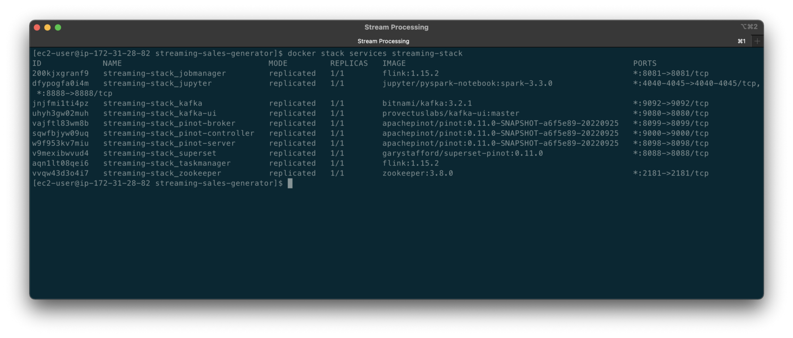
New Streaming Stack

To get started, we need to replace the first streaming Docker Swarm stack, deployed in part one, with the second streaming Docker Swarm stack. The second stack contains Apache Kafka, Apache Zookeeper, Apache Flink, Apache Pinot, Apache Superset, UI for Apache Kafka, and Project Jupyter (JupyterLab).

https://programmaticponderings.wordpress.com/media/601efca17604c3a467a4200e93d7d3ff

The stack will take a few minutes to deploy fully. When complete, there should be ten containers running in the stack.

Viewing the Docker streaming stack’s ten containers

Flink Application

The Flink application has two entry classes. The first class, RunningTotals, performs an identical aggregation function as the previous KStreams demo.

	public static void flinkKafkaPipeline(Properties prop) throws Exception {
	StreamExecutionEnvironment env = StreamExecutionEnvironment.getExecutionEnvironment();

	// assumes PLAINTEXT authentication
	KafkaSource<Purchase> source = KafkaSource.<Purchase>builder()
	.setBootstrapServers(prop.getProperty("BOOTSTRAP_SERVERS"))
	.setTopics(prop.getProperty("PURCHASES_TOPIC"))
	.setGroupId("flink_reduce_demo")
	.setStartingOffsets(OffsetsInitializer.earliest())
	.setValueOnlyDeserializer(new PurchaseDeserializationSchema())
	.build();

	DataStream<Purchase> purchases = env.fromSource(source, WatermarkStrategy.noWatermarks(), "Kafka Source");

	DataStream<RunningTotal> runningTotals = purchases
	.flatMap((FlatMapFunction<Purchase, RunningTotal>) (purchase, out) -> out.collect(
	new RunningTotal(
	purchase.getTransactionTime(),
	purchase.getProductId(),
	1,
	purchase.getQuantity(),
	purchase.getTotalPurchase()
	))
	).returns(RunningTotal.class)
	.keyBy(RunningTotal::getProductId)
	.reduce((runningTotal1, runningTotal2) -> {
	runningTotal2.setTransactions(runningTotal1.getTransactions() + runningTotal2.getTransactions());
	runningTotal2.setQuantities(runningTotal1.getQuantities() + runningTotal2.getQuantities());
	runningTotal2.setSales(runningTotal1.getSales().add(runningTotal2.getSales()));
	return runningTotal2;
	});

	KafkaSink<RunningTotal> sink = KafkaSink.<RunningTotal>builder()
	.setBootstrapServers(prop.getProperty("BOOTSTRAP_SERVERS"))
	.setRecordSerializer(KafkaRecordSerializationSchema.builder()
	.setTopic(prop.getProperty("RUNNING_TOTALS_TOPIC"))
	.setValueSerializationSchema(new RunningTotalSerializationSchema())
	.build()
	).setDeliveryGuarantee(DeliveryGuarantee.AT_LEAST_ONCE)
	.build();

	runningTotals.sinkTo(sink);

	env.execute("Flink Running Totals Demo");
	}

view raw RunningTotals.java hosted with ❤ by GitHub

The second class, JoinStreams, joins the stream of data from the demo.purchases topic and the demo.products topic, processing and combining them, in real-time, into an enriched transaction and publishing the results to a new topic, demo.purchases.enriched.

	public static void flinkKafkaPipeline(Properties prop) throws Exception {
	StreamExecutionEnvironment env = StreamExecutionEnvironment.getExecutionEnvironment();
	StreamTableEnvironment tableEnv = StreamTableEnvironment.create(env);

	// assumes PLAINTEXT authentication
	KafkaSource<Product> productSource = KafkaSource.<Product>builder()
	.setBootstrapServers(prop.getProperty("BOOTSTRAP_SERVERS"))
	.setTopics(prop.getProperty("PRODUCTS_TOPIC"))
	.setGroupId("flink_join_demo")
	.setStartingOffsets(OffsetsInitializer.earliest())
	.setValueOnlyDeserializer(new ProductDeserializationSchema())
	.build();

	DataStream<Product> productsStream = env.fromSource(
	productSource, WatermarkStrategy.noWatermarks(), "Kafka Products Source");

	tableEnv.createTemporaryView("products", productsStream);

	KafkaSource<Purchase> purchasesSource = KafkaSource.<Purchase>builder()
	.setBootstrapServers(prop.getProperty("BOOTSTRAP_SERVERS"))
	.setTopics(prop.getProperty("PURCHASES_TOPIC"))
	.setGroupId("flink_join_demo")
	.setStartingOffsets(OffsetsInitializer.earliest())
	.setValueOnlyDeserializer(new PurchaseDeserializationSchema())
	.build();

	DataStream<Purchase> purchasesStream = env.fromSource(
	purchasesSource, WatermarkStrategy.noWatermarks(), "Kafka Purchases Source");

	tableEnv.createTemporaryView("purchases", purchasesStream);

	Table result =
	tableEnv.sqlQuery(
	"SELECT " +
	"purchases.transactionTime, " +
	"TO_TIMESTAMP(purchases.transactionTime), " +
	"purchases.transactionId, " +
	"purchases.productId, " +
	"products.category, " +
	"products.item, " +
	"products.size, " +
	"products.cogs, " +
	"products.price, " +
	"products.containsFruit, " +
	"products.containsVeggies, " +
	"products.containsNuts, " +
	"products.containsCaffeine, " +
	"purchases.price, " +
	"purchases.quantity, " +
	"purchases.isMember, " +
	"purchases.memberDiscount, " +
	"purchases.addSupplements, " +
	"purchases.supplementPrice, " +
	"purchases.totalPurchase " +
	"FROM " +
	"products " +
	"JOIN purchases " +
	"ON products.productId = purchases.productId"
	);

	DataStream<PurchaseEnriched> purchasesEnrichedTable = tableEnv.toDataStream(result,
	PurchaseEnriched.class);

	KafkaSink<PurchaseEnriched> sink = KafkaSink.<PurchaseEnriched>builder()
	.setBootstrapServers(prop.getProperty("BOOTSTRAP_SERVERS"))
	.setRecordSerializer(KafkaRecordSerializationSchema.builder()
	.setTopic(prop.getProperty("PURCHASES_ENRICHED_TOPIC"))
	.setValueSerializationSchema(new PurchaseEnrichedSerializationSchema())
	.build()
	).setDeliveryGuarantee(DeliveryGuarantee.AT_LEAST_ONCE)
	.build();

	purchasesEnrichedTable.sinkTo(sink);

	env.execute("Flink Streaming Join Demo");
	}

view raw JoinStreams.java hosted with ❤ by GitHub

The resulting enriched purchases messages look similar to the following:

	{
	"transaction_time": "2022-09-25 01:58:11.714838",
	"transaction_id": "4068565608708439642",
	"product_id": "CS08",
	"product_category": "Classic Smoothies",
	"product_name": "Rockin’ Raspberry",
	"product_size": "24 oz.",
	"product_cogs": 1.5,
	"product_price": 4.99,
	"contains_fruit": true,
	"contains_veggies": false,
	"contains_nuts": false,
	"contains_caffeine": false,
	"purchase_price": 4.99,
	"purchase_quantity": 2,
	"is_member": false,
	"member_discount": 0,
	"add_supplements": false,
	"supplement_price": 0,
	"total_purchase": 9.98
	}

view raw enriched_purchase.json hosted with ❤ by GitHub

Sample enriched purchase message

Running the Flink Job

To run the Flink application, we must first compile it into an uber JAR.

	# set java version (v11 is latest compatible version with Apache Flink)
	JAVA_HOME=~/Library/Java/JavaVirtualMachines/corretto-11.0.16.1/Contents/Home

	# compile to uber jar
	./gradlew clean shadowJar

view raw build_flink_app.sh hosted with ❤ by GitHub

We can copy the JAR into the Flink container or upload it through the Apache Flink Dashboard, a browser-based UI. For this demonstration, we will upload it through the Apache Flink Dashboard, accessible on port 8081.

The project’s build.gradle file has preset the Main class (Flink’s Entry class) to org.example.JoinStreams. Optionally, to run the Running Totals demo, we could change the build.gradle file and recompile, or simply change Flink’s Entry class to org.example.RunningTotals.

Before running the Flink job, restart the sales generator in the background (nohup python3 ./producer.py &) to generate a new stream of data. Then start the Flink job.

To confirm the Flink application is running, we can check the contents of the new demo.purchases.enriched topic using the Kafka CLI.

	# establish an interactive session with the kafka container
	KAFKA_CONTAINER=$(docker container ls –filter name=streaming-stack_kafka.1 –format "{{.ID}}")
	docker exec -it ${KAFKA_CONTAINER} bash

	# set environment variables used by jobs
	export BOOTSTRAP_SERVERS="localhost:9092"
	export OUTPUT_TOPIC="demo.purchases.enriched";

	# read topics from beginning
	kafka-console-consumer.sh \
	–topic $OUTPUT_TOPIC –from-beginning \
	–bootstrap-server $BOOTSTRAP_SERVERS

view raw consume_flink_job.sh hosted with ❤ by GitHub

The new demo.purchases.enriched topic populated with messages from Apache Flink

Alternatively, you can use the UI for Apache Kafka, accessible on port 9080.

Viewing messages in the UI for Apache Kafka

Demonstration #4: Apache Pinot

In the fourth and final demonstration, we will explore Apache Pinot. First, we will query the unbounded data streams from Apache Kafka, generated by both the sales generator and the Apache Flink application, using SQL. Then, we build a real-time dashboard in Apache Superset, with Apache Pinot as our datasource.

Creating Tables

According to the Apache Pinot documentation, “a table is a logical abstraction that represents a collection of related data. It is composed of columns and rows (known as documents in Pinot).” There are three types of Pinot tables: Offline, Realtime, and Hybrid. For this demonstration, we will create three Realtime tables. Realtime tables ingest data from streams — in our case, Kafka — and build segments from the consumed data. Further, according to the documentation, “each table in Pinot is associated with a Schema. A schema defines what fields are present in the table along with the data types. The schema is stored in Zookeeper, along with the table configuration.”

Below, we see the schema and config for one of the three Realtime tables, purchasesEnriched. Note how the columns are divided into three categories: Dimension, Metric, and DateTime.

	{
	"schemaName": "purchasesEnriched",
	"dimensionFieldSpecs": [
	{
	"name": "transaction_id",
	"dataType": "STRING"
	},
	{
	"name": "product_id",
	"dataType": "STRING"
	},
	{
	"name": "product_category",
	"dataType": "STRING"
	},
	{
	"name": "product_name",
	"dataType": "STRING"
	},
	{
	"name": "product_size",
	"dataType": "STRING"
	},
	{
	"name": "product_cogs",
	"dataType": "FLOAT"
	},
	{
	"name": "product_price",
	"dataType": "FLOAT"
	},
	{
	"name": "contains_fruit",
	"dataType": "BOOLEAN"
	},
	{
	"name": "contains_veggies",
	"dataType": "BOOLEAN"
	},
	{
	"name": "contains_nuts",
	"dataType": "BOOLEAN"
	},
	{
	"name": "contains_caffeine",
	"dataType": "BOOLEAN"
	},
	{
	"name": "purchase_price",
	"dataType": "FLOAT"
	},
	{
	"name": "is_member",
	"dataType": "BOOLEAN"
	},
	{
	"name": "member_discount",
	"dataType": "FLOAT"
	},
	{
	"name": "add_supplements",
	"dataType": "BOOLEAN"
	},
	{
	"name": "supplement_price",
	"dataType": "FLOAT"
	}
	],
	"metricFieldSpecs": [
	{
	"name": "purchase_quantity",
	"dataType": "INT"
	},
	{
	"name": "total_purchase",
	"dataType": "FLOAT"
	}
	],
	"dateTimeFieldSpecs": [
	{
	"name": "transaction_time",
	"dataType": "TIMESTAMP",
	"format": "1:MILLISECONDS:SIMPLE_DATE_FORMAT:yyyy-MM-dd HH:mm:ss.SSSSSS",
	"granularity": "1:MILLISECONDS"
	}
	]
	}

view raw purchases-enriched-schema.json hosted with ❤ by GitHub

Schema file for purchasesEnriched Realtime table

	{
	"tableName": "purchasesEnriched",
	"tableType": "REALTIME",
	"segmentsConfig": {
	"timeColumnName": "transaction_time",
	"timeType": "MILLISECONDS",
	"schemaName": "purchasesEnriched",
	"replicasPerPartition": "1"
	},
	"tenants": {},
	"tableIndexConfig": {
	"loadMode": "MMAP",
	"streamConfigs": {
	"streamType": "kafka",
	"stream.kafka.consumer.type": "lowlevel",
	"stream.kafka.topic.name": "demo.purchases.enriched",
	"stream.kafka.decoder.class.name": "org.apache.pinot.plugin.stream.kafka.KafkaJSONMessageDecoder",
	"stream.kafka.consumer.factory.class.name": "org.apache.pinot.plugin.stream.kafka20.KafkaConsumerFactory",
	"stream.kafka.broker.list": "kafka:29092",
	"realtime.segment.flush.threshold.time": "3600000",
	"realtime.segment.flush.threshold.rows": "50000",
	"stream.kafka.consumer.prop.auto.offset.reset": "smallest"
	}
	},
	"metadata": {}
	}

view raw purchases-enriched-config.json hosted with ❤ by GitHub

Config file for purchasesEnriched Realtime table

To begin, copy the three Pinot Realtime table schemas and configurations from the streaming-sales-generator GitHub project into the Apache Pinot Controller container. Next, use a docker exec command to call the Pinot Command Line Interface’s (CLI) AddTable command to create the three tables: products, purchases, and purchasesEnriched.

	# copy pinot table schema and config files to pinot controller
	CONTROLLER_CONTAINER=$(docker container ls –filter name=streaming-stack_pinot-controller.1 –format "{{.ID}}")
	cd ~/streaming-sales-generator/apache_pinot_examples
	docker cp configs_schemas/ ${CONTROLLER_CONTAINER}:/tmp/

	# create three tables
	docker exec -it ${CONTROLLER_CONTAINER} \
	bin/pinot-admin.sh AddTable \
	-tableConfigFile /tmp/configs_schemas/purchases-config.json \
	-schemaFile /tmp/configs_schemas/purchases-schema.json -exec

	docker exec -it ${CONTROLLER_CONTAINER} \
	bin/pinot-admin.sh AddTable \
	-tableConfigFile /tmp/configs_schemas/products-config.json \
	-schemaFile /tmp/configs_schemas/products-schema.json -exec

	docker exec -it ${CONTROLLER_CONTAINER} \
	bin/pinot-admin.sh AddTable \
	-tableConfigFile /tmp/configs_schemas/purchases-enriched-config.json \
	-schemaFile /tmp/configs_schemas/purchases-enriched-schema.json -exec

view raw create_new_tables.sh hosted with ❤ by GitHub

To confirm the three tables were created correctly, use the Apache Pinot Data Explorer accessible on port 9000. Use the Tables tab in the Cluster Manager.

Cluster Manager’s Tables tab shows the three Realtime tables and corresponding schemas

We can further inspect and edit the table’s config and schema from the Tables tab in the Cluster Manager.

Realtime table’s editable config and schema

The three tables are configured to read the unbounded stream of data from the corresponding Kafka topics: demo.products, demo.purchases, and demo.purchases.enriched.

Querying with Pinot

We can use Pinot’s Query Console to query the Realtime tables using SQL. According to the documentation, “Pinot provides a SQL interface for querying. It uses the [Apache] Calcite SQL parser to parse queries and uses MYSQL_ANSI dialect.”

Schema and query results for the purchases table

With the generator still running, re-query the purchases table in the Query Console (select count(*) from purchases). You should notice the document count increasing each time you re-run the query since new messages are published to the demo.purchases topic by the sales generator.

If you do not observe the count increasing, ensure the sales generator and Flink enrichment job are running.

Query Console showing the purchases table’s document count continuing to increase

Table Joins?

It might seem logical to want to replicate the same multi-stream join we performed with Apache Flink in part three of the demonstration on the demo.products and demo.purchases topics. Further, we might presume to join the products and purchases realtime tables by writing a SQL statement in Pinot’s Query Console. However, according to the documentation, at the time of this post, version 0.11.0 of Pinot did not [currently] support joins or nested subqueries.

This current join limitation is why we created the Realtime table, purchasesEnriched, allowing us to query Flink’s real-time results in the demo.purchases.enriched topic. We will use both Flink and Pinot as part of our stream processing pipeline, taking advantage of each tool’s individual strengths and capabilities.

Note, according to the documentation for the latest release of Pinot on the main branch, “the latest Pinot multi-stage supports inner join, left-outer, semi-join, and nested queries out of the box. It is optimized for in-memory process and latency.” For more information on joins as part of Pinot’s new multi-stage query execution engine, read the documentation, Multi-Stage Query Engine.

Query showing results from the `demo.purchases.enriched` topic in real-time

Aggregations

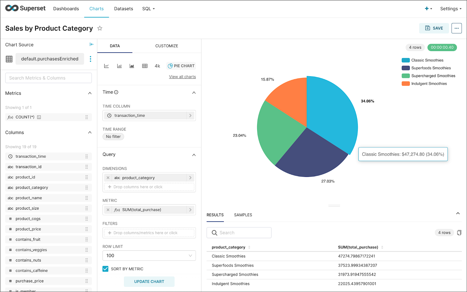
We can perform real-time aggregations using Pinot’s rich SQL query interface. For example, like previously with Spark and Flink, we can calculate running totals for the number of items sold and the total sales for each product in real time.

Aggregating running totals for each product

We can do the same with the purchasesEnriched table, which will use the continuous stream of enriched transaction data from our Apache Flink application. With the purchasesEnriched table, we can add the product name and product category for richer results. Each time we run the query, we get real-time results based on the running sales generator and Flink enrichment job.

Query Options and Indexing

Note the reference to the Star-Tree index at the start of the SQL query shown above. Pinot provides several query options, including useStarTree (true by default).

Multiple indexing techniques are available in Pinot, including Forward Index, Inverted Index, Star-tree Index, Bloom Filter, and Range Index, among others. Each has advantages in different query scenarios. According to the documentation, by default, Pinot creates a dictionary-encoded forward index for each column.

SQL Examples

Here are a few examples of SQL queries you can try in Pinot’s Query Console:

	— products
	SELECT
	COUNT(product_id) AS product_count,
	AVG(price) AS avg_price,
	AVG(cogs) AS avg_cogs,
	AVG(price) – AVG(cogs) AS avg_gross_profit
	FROM
	products;

	— purchases
	SELECT
	product_id,
	SUMPRECISION(quantity, 10, 0) AS quantity,
	SUMPRECISION(total_purchase, 10, 2) AS sales
	FROM
	purchases
	GROUP BY
	product_id
	ORDER BY
	sales DESC;

	— purchasesEnriched
	SELECT
	product_id,
	product_name,
	product_category,
	SUMPRECISION(purchase_quantity, 10, 0) AS quantity,
	SUMPRECISION(total_purchase, 10, 2) AS sales
	FROM
	purchasesEnriched
	GROUP BY
	product_id,
	product_name,
	product_category
	ORDER BY
	sales DESC;

view raw pinot_sql_example.sql hosted with ❤ by GitHub

Troubleshooting Pinot

If have issues with creating the tables or querying the real-time data, you can start by reviewing the Apache Pinot logs:

	CONTROLLER_CONTAINER=$(docker container ls –filter name=streaming-stack_pinot-controller.1 –format "{{.ID}}")
	docker exec -it ${CONTROLLER_CONTAINER} cat logs/pinot-all.log

view raw pinot_logs.sh hosted with ❤ by GitHub

Real-time Dashboards with Apache Superset

To display the real-time stream of data produced results of our Apache Flink stream processing job and made queriable by Apache Pinot, we can use Apache Superset. Superset positions itself as “a modern data exploration and visualization platform.” Superset allows users “to explore and visualize their data, from simple line charts to highly detailed geospatial charts.”

According to the documentation, “Superset requires a Python DB-API database driver and a SQLAlchemy dialect to be installed for each datastore you want to connect to.” In the case of Apache Pinot, we can use pinotdb as the Python DB-API and SQLAlchemy dialect for Pinot. Since the existing Superset Docker container does not have pinotdb installed, I have built and published a Docker Image with the driver and deployed it as part of the second streaming stack of containers.

	# Custom Superset build to add apache pinot driver
	# Gary A. Stafford (2022-09-25)
	# Updated: 2022-12-18

	FROM apache/superset:66138b0ca0b82a94404e058f0cc55517b2240069

	# Switching to root to install the required packages
	USER root

	# Find which driver you need based on the analytics database:
	# https://superset.apache.org/docs/databases/installing-database-drivers
	RUN pip install mysqlclient psycopg2-binary pinotdb

	# Switching back to using the `superset` user
	USER superset

view raw Dockerfile hosted with ❤ by GitHub

First, we much configure the Superset container instance. These instructions are documented as part of the Superset Docker Image repository.

	# establish an interactive session with the superset container
	SUPERSET_CONTAINER=$(docker container ls –filter name=streaming-stack_superset.1 –format "{{.ID}}")

	# initialize superset (see superset documentation)
	docker exec -it ${SUPERSET_CONTAINER} \
	superset fab create-admin \
	–username admin \
	–firstname Superset \
	–lastname Admin \
	–email admin@superset.com \
	–password sUp3rS3cREtPa55w0rD1

	docker exec -it ${SUPERSET_CONTAINER} superset db upgrade

	docker exec -it ${SUPERSET_CONTAINER} superset init

view raw initialize_superset.sh hosted with ❤ by GitHub

Once the configuration is complete, we can log into the Superset web-browser-based UI accessible on port 8088.

Home page of the Superset web-browser-based UI

Pinot Database Connection and Dataset

Next, to connect to Pinot from Superset, we need to create a Database Connection and a Dataset.

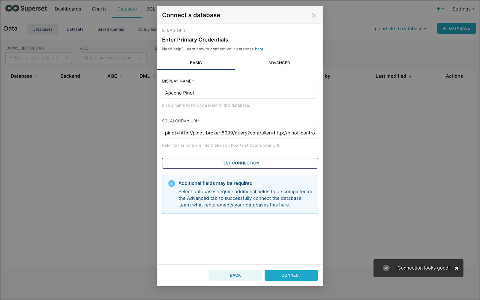
Creating a new database connection to Pinot

The SQLAlchemy URI is shown below. Input the URI, test your connection (‘Test Connection’), make sure it succeeds, then hit ‘Connect’.

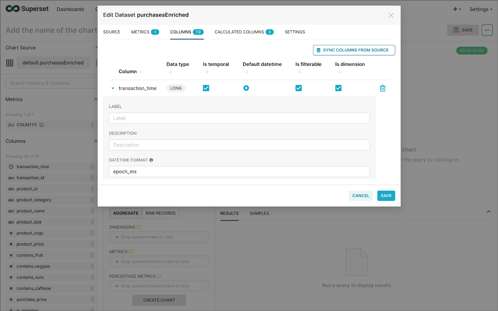
pinot+http://pinot-broker:8099/query?controller=http://pinot-controller:9000

view raw pinot_superset_conn.txt hosted with ❤ by GitHub

Next, create a Dataset that references the purchasesEnriched Pinot table.

Creating a new dataset allowing us access to the `purchasesEnriched` Pinot table

Modify the dataset’s transaction_time column. Check the is_temporal and Default datetime options. Lastly, define the DateTime format as epoch_ms.

Modifying the dataset’s `transaction_time` column

Building a Real-time Dashboard

Using the new dataset, which connects Superset to the purchasesEnriched Pinot table, we can construct individual charts to be placed on a dashboard. Build a few charts to include on your dashboard.

Example of a chart whose data source is the new dataset

List of charts that included on the dashboard

Create a new Superset dashboard and add the charts and other elements, such as headlines, dividers, and tabs.

Apache Superset dashboard displaying data from Apache Pinot Realtime table

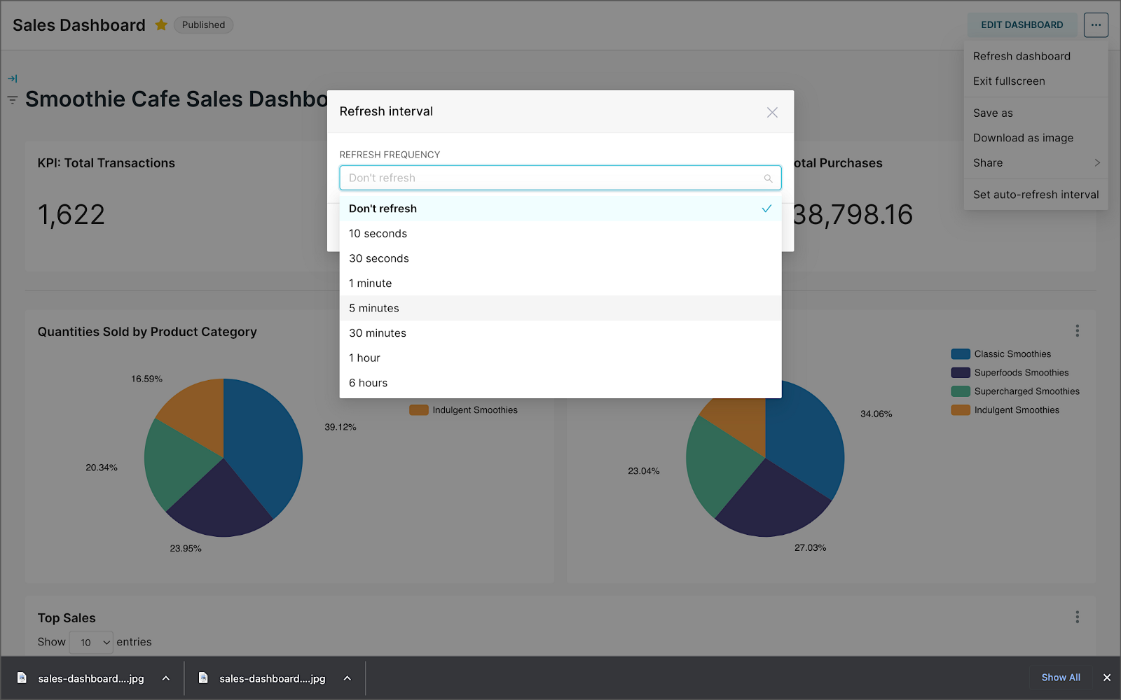
We can apply a refresh interval to the dashboard to continuously query Pinot and visualize the results in near real-time.

Configuring a refresh interval for the dashboard

Conclusion

In this two-part post series, we were introduced to stream processing. We explored four popular open-source stream processing projects: Apache Spark Structured Streaming, Apache Kafka Streams, Apache Flink, and Apache Pinot. Next, we learned how we could solve similar stream processing and streaming analytics challenges using different streaming technologies. Lastly, we saw how these technologies, such as Kafka, Flink, Pinot, and Superset, could be integrated to create effective stream processing pipelines.

This blog represents my viewpoints and not of my employer, Amazon Web Services (AWS). All product names, logos, and brands are the property of their respective owners. All diagrams and illustrations are the property of the author unless otherwise noted.

Apache Flink, Apache Kafka, Apache Kafka Streams, Apache Pinot, Apache Spark, Apache Superset, Data Analytics, Stream Processing, Streaming Analytics, Streaming data

Exploring Popular Open-source Stream Processing Technologies: Part 1 of 2

Posted by Gary A. Stafford in Analytics, Big Data, Java Development, Python, Software Development, SQL on September 24, 2022

A brief demonstration of Apache Spark Structured Streaming, Apache Kafka Streams, Apache Flink, and Apache Pinot with Apache Superset

Introduction

Batch vs. Stream Processing

Again, according to Confluent, “Batch processing is when the processing and analysis happens on a set of data that have already been stored over a period of time.” A batch processing example might include daily retail sales data, which is aggregated and tabulated nightly after the stores close. Conversely, “streaming data processing happens as the data flows through a system. This results in analysis and reporting of events as it happens.” To use a similar example, instead of nightly batch processing, the streams of sales data are processed, aggregated, and analyzed continuously throughout the day — sales volume, buying trends, inventory levels, and marketing program performance are tracked in real time.

Bounded vs. Unbounded Data

According to Packt Publishing’s book, Learning Apache Apex, “bounded data is finite; it has a beginning and an end. Unbounded data is an ever-growing, essentially infinite data set.” Batch processing is typically performed on bounded data, whereas stream processing is most often performed on unbounded data.

Stream Processing Technologies

There are many technologies available to perform stream processing. These include proprietary custom software, commercial off-the-shelf (COTS) software, fully-managed service offerings from Software as a Service (or SaaS) providers, Cloud Solution Providers (CSP), Commercial Open Source Software (COSS) companies, and popular open-source projects from the Apache Software Foundation and Linux Foundation.

The following two-part post and forthcoming video will explore four popular open-source software (OSS) stream processing projects, including Apache Spark Structured Streaming, Apache Kafka Streams, Apache Flink, and Apache Pinot. Each of these projects has some equivalent SaaS, CSP, and COSS offerings.

Apache Spark Structured Streaming

According to the Apache Spark documentation, “Structured Streaming is a scalable and fault-tolerant stream processing engine built on the Spark SQL engine. You can express your streaming computation the same way you would express a batch computation on static data.” Further, “Structured Streaming queries are processed using a micro-batch processing engine, which processes data streams as a series of small batch jobs thereby achieving end-to-end latencies as low as 100 milliseconds and exactly-once fault-tolerance guarantees.” In the post, we will examine both batch and stream processing using a series of Apache Spark Structured Streaming jobs written in PySpark.

Spark Structured Streaming job statistics as seen from the Spark UI

Apache Kafka Streams

According to the Apache Kafka documentation, “Kafka Streams [aka KStreams] is a client library for building applications and microservices, where the input and output data are stored in Kafka clusters. It combines the simplicity of writing and deploying standard Java and Scala applications on the client side with the benefits of Kafka’s server-side cluster technology.” In the post, we will examine a KStreams application written in Java that performs stream processing and incremental aggregation.

Building the KStreams application’s uber JAR in JetBrains IntelliJ IDEA

Apache Flink

According to the Apache Flink documentation, “Apache Flink is a framework and distributed processing engine for stateful computations over unbounded and bounded data streams. Flink has been designed to run in all common cluster environments, perform computations at in-memory speed and at any scale.” Further, “Apache Flink excels at processing unbounded and bounded data sets. Precise control of time and state enables Flink’s runtime to run any kind of application on unbounded streams. Bounded streams are internally processed by algorithms and data structures that are specifically designed for fixed-sized data sets, yielding excellent performance.” In the post, we will examine a Flink application written in Java, which performs stream processing, incremental aggregation, and multi-stream joins.

Apache Pinot

According to Apache Pinot’s documentation, “Pinot is a real-time distributed OLAP datastore, purpose-built to provide ultra-low-latency analytics, even at extremely high throughput. It can ingest directly from streaming data sources — such as Apache Kafka and Amazon Kinesis — and make the events available for querying instantly. It can also ingest from batch data sources such as Hadoop HDFS, Amazon S3, Azure ADLS, and Google Cloud Storage.” In the post, we will query the unbounded data streams from Apache Kafka, generated by Apache Flink, using SQL.

Streaming Data Source

We must first find a good unbounded data source to explore or demonstrate these streaming technologies. Ideally, the streaming data source should be complex enough to allow multiple types of analyses and visualize different aspects with Business Intelligence (BI) and dashboarding tools. Additionally, the streaming data source should possess a degree of consistency and predictability while displaying a reasonable level of variability and randomness.

To this end, we will use the open-source Streaming Synthetic Sales Data Generator project, which I have developed and made available on GitHub. This project’s highly-configurable, Python-based, synthetic data generator generates an unbounded stream of product listings, sales transactions, and inventory restocking activities to a series of Apache Kafka topics.

Streaming Synthetic Sales Data Generator publishing messages to Apache Kafka

Source Code

All the source code demonstrated in this post is open source and available on GitHub. There are three separate GitHub projects:

	# streaming data generator, Apache Spark and Apache Pinot examples
	git clone –depth 1 -b main \
	https://github.com/garystafford/streaming-sales-generator.git

	# Apache Flink examples
	git clone –depth 1 -b main \
	https://github.com/garystafford/flink-kafka-demo.git

	# Kafka Streams examples
	git clone –depth 1 -b main \
	https://github.com/garystafford/kstreams-kafka-demo.git

view raw github_projects.sh hosted with ❤ by GitHub

Docker

To make it easier to follow along with the demonstration, we will use Docker Swarm to provision the streaming tools. Alternatively, you could use Kubernetes (e.g., creating a Helm chart) or your preferred CSP or SaaS managed services. Nothing in this demonstration requires you to use a paid service.

The two Docker Swarm stacks are located in the Streaming Synthetic Sales Data Generator project:

Streaming Stack — Part 1: Apache Kafka, Apache Zookeeper, Apache Spark, UI for Apache Kafka, and the KStreams application
Streaming Stack — Part 2: Apache Kafka, Apache Zookeeper, Apache Flink, Apache Pinot, Apache Superset, UI for Apache Kafka, and Project Jupyter (JupyterLab).*

* the Jupyter container can be used as an alternative to the Spark container for running PySpark jobs (follow the same steps as for Spark, below)

Demonstration #1: Apache Spark

In the first of four demonstrations, we will examine two Apache Spark Structured Streaming jobs, written in PySpark, demonstrating both batch processing (spark_batch_kafka.py) and stream processing (spark_streaming_kafka.py). We will read from a single stream of data from a Kafka topic, demo.purchases, and write to the console.

High-level workflow for Apache Spark demonstration

Deploying the Streaming Stack

To get started, deploy the first streaming Docker Swarm stack containing the Apache Kafka, Apache Zookeeper, Apache Spark, UI for Apache Kafka, and the KStreams application containers.

	# cd into project
	cd streaming-sales-generator/

	# initialize swarm stack – 1x only
	docker swarm init

	# optional: delete previous streaming-stack
	docker stack rm streaming-stack

	# deploy first streaming-stack
	docker stack deploy streaming-stack –compose-file docker/spark-kstreams-stack.yml

	# observe the deployment's progress
	docker stack services streaming-stack

view raw deploy_streaming_stack_1.sh hosted with ❤ by GitHub

The stack will take a few minutes to deploy fully. When complete, there should be a total of six containers running in the stack.

Viewing the Docker streaming stack’s six containers

Sales Generator

Before starting the streaming data generator, confirm or modify the configuration/configuration.ini. Three configuration items, in particular, will determine how long the streaming data generator runs and how much data it produces. We will set the timing of transaction events to be generated relatively rapidly for test purposes. We will also set the number of events high enough to give us time to explore the Spark jobs. Using the below settings, the generator should run for an average of approximately 50–60 minutes: (((5 sec + 2 sec)/2)*1000 transactions)/60 sec=~58 min on average. You can run the generator again if necessary or increase the number of transactions.

	[SALES]
	# minimum sales frequency in seconds (debug with 1, typical min. 120)
	min_sale_freq = 2

	# maximum sales frequency in seconds (debug with 3, typical max. 300)
	max_sale_freq = 5

	# number of transactions to generate
	number_of_sales = 1000

view raw configuration.ini hosted with ❤ by GitHub

A code snippet from the project’s configuration.ini file

Start the streaming data generator as a background service:

	# install required python packages (1x)
	python3 -m pip install kafka-python

	cd sales_generator/

	# run in foreground
	python3 ./producer.py

	# better option, run as background process
	nohup python3 ./producer.py &

	# confirm process is running
	ps -u

view raw run_sales_generator.sh hosted with ❤ by GitHub

The streaming data generator will start writing data to three Apache Kafka topics: demo.products, demo.purchases, and demo.inventories. We can view these topics and their messages by logging into the Apache Kafka container and using the Kafka CLI:

	# establish an interactive session with the spark container
	KAFKA_CONTAINER=$(docker container ls –filter name=streaming-stack_kafka.1 –format "{{.ID}}")
	docker exec -it ${KAFKA_CONTAINER} bash

	# set environment variables used by jobs
	export BOOTSTRAP_SERVERS="localhost:9092"
	export TOPIC_PRODUCTS="demo.products"
	export TOPIC_PURCHASES="demo.purchases"
	export TOPIC_INVENTORIES="demo.inventories"

	# list topics
	kafka-topics.sh –list –bootstrap-server $BOOTSTRAP_SERVERS

	# read topics from beginning
	kafka-console-consumer.sh \
	–topic $TOPIC_PRODUCTS –from-beginning \
	–bootstrap-server $BOOTSTRAP_SERVERS

	kafka-console-consumer.sh \
	–topic $TOPIC_PURCHASES –from-beginning \
	–bootstrap-server $BOOTSTRAP_SERVERS

	kafka-console-consumer.sh \
	–topic $TOPIC_INVENTORIES –from-beginning \
	–bootstrap-server $BOOTSTRAP_SERVERS

view raw read_kafka_topics.sh hosted with ❤ by GitHub

Below, we see a few sample messages from the demo.purchases topic:

Consuming messages from Kafka’s `demo.purchases` topic

Alternatively, you can use the UI for Apache Kafka, accessible on port 9080.

Viewing `demo.purchases` topic in the UI for Apache Kafka

Viewing messages in the `demo.purchases` topic using the UI for Apache Kafka

Prepare Spark

Next, prepare the Spark container to run the Spark jobs:

	# establish an interactive session with the spark container
	SPARK_CONTAINER=$(docker container ls –filter name=streaming-stack_spark.1 –format "{{.ID}}")
	docker exec -it -u 0 ${SPARK_CONTAINER} bash

	# update and install wget
	apt-get update && apt-get install wget vim -y

	# install required job dependencies
	wget https://repo1.maven.org/maven2/org/apache/commons/commons-pool2/2.11.1/commons-pool2-2.11.1.jar
	wget https://repo1.maven.org/maven2/org/apache/kafka/kafka-clients/3.3.1/kafka-clients-3.3.1.jar
	wget https://repo1.maven.org/maven2/org/apache/spark/spark-sql-kafka-0-10_2.12/3.3.1/spark-sql-kafka-0-10_2.12-3.3.1.jar
	wget https://repo1.maven.org/maven2/org/apache/spark/spark-token-provider-kafka-0-10_2.12/3.3.1/spark-token-provider-kafka-0-10_2.12-3.3.1.jar
	mv *.jar /opt/bitnami/spark/jars/

	exit

view raw prepare_spark_container.sh hosted with ❤ by GitHub

Preparing the Spark container instance as the root user

Running the Spark Jobs

Next, copy the jobs from the project to the Spark container, then exec back into the container:

	# copy jobs to spark container
	docker cp apache_spark_examples/ ${SPARK_CONTAINER}:/home/

	# establish an interactive session with the spark container
	docker exec -it ${SPARK_CONTAINER} bash

view raw run_spark_jobs.sh hosted with ❤ by GitHub

Batch Processing with Spark

The first Spark job, spark_batch_kafka.py, aggregates the number of items sold and the total sales for each product, based on existing messages consumed from the demo.purchases topic. We use the PySpark DataFrame class’s read() and write() methods in the first example, reading from Kafka and writing to the console. We could just as easily write the results back to Kafka.

	ds_sales = (
	df_sales.selectExpr("CAST(value AS STRING)")
	.select(F.from_json("value", schema=schema).alias("data"))
	.select("data.*")
	.withColumn("row", F.row_number().over(window))
	.withColumn("quantity", F.sum(F.col("quantity")).over(window_agg))
	.withColumn("sales", F.sum(F.col("total_purchase")).over(window_agg))
	.filter(F.col("row") == 1)
	.drop("row")
	.select(
	"product_id",
	F.format_number("sales", 2).alias("sales"),
	F.format_number("quantity", 0).alias("quantity"),
	)
	.coalesce(1)
	.orderBy(F.regexp_replace("sales", ",", "").cast("float"), ascending=False)
	.write.format("console")
	.option("numRows", 25)
	.option("truncate", False)
	.save()
	)

view raw spark_batch_snippet.py hosted with ❤ by GitHub

A snippet of batch processing Spark job’s summarize_sales() method

The batch processing job sorts the results and outputs the top 25 items by total sales to the console. The job should run to completion and exit successfully.

Batch results for top 25 items by total sales

To run the batch Spark job, use the following commands:

	# set environment variables used by jobs
	export BOOTSTRAP_SERVERS="kafka:29092"
	export TOPIC_PURCHASES="demo.purchases"

	cd /home/apache_spark_examples/

	# run batch processing job
	spark-submit spark_batch_kafka.py

view raw run_spark_batch.sh hosted with ❤ by GitHub

Run the batch Spark job

Stream Processing with Spark

The stream processing Spark job, spark_streaming_kafka.py, also aggregates the number of items sold and the total sales for each item, based on messages consumed from the demo.purchases topic. However, as shown in the code snippet below, this job continuously aggregates the stream of data from Kafka, displaying the top ten product totals within an arbitrary ten-minute sliding window, with a five-minute overlap, and updates output every minute to the console. We use the PySpark DataFrame class’s readStream() and writeStream() methods as opposed to the batch-oriented read() and write() methods in the first example.

	ds_sales = (
	df_sales.selectExpr("CAST(value AS STRING)")
	.select(F.from_json("value", schema=schema).alias("data"))
	.select("data.*")
	.withWatermark("transaction_time", "10 minutes")
	.groupBy("product_id", F.window("transaction_time", "10 minutes", "5 minutes"))
	.agg(F.sum("total_purchase"), F.sum("quantity"))
	.orderBy(F.col("window").desc(), F.col("sum(total_purchase)").desc())
	.select(
	"product_id",
	F.format_number("sum(total_purchase)", 2).alias("sales"),
	F.format_number("sum(quantity)", 0).alias("drinks"),
	"window.start",
	"window.end",
	)
	.coalesce(1)
	.writeStream.queryName("streaming_to_console")
	.trigger(processingTime="1 minute")
	.outputMode("complete")
	.format("console")
	.option("numRows", 10)
	.option("truncate", False)
	.start()
	)

	ds_sales.awaitTermination()

view raw spark_streaming_snippet.py hosted with ❤ by GitHub

A snippet of stream processing Spark job’s summarize_sales() method

Shorter event-time windows are easier for demonstrations — in Production, hourly, daily, weekly, or monthly windows are more typical for sales analysis.

Micro-batch representing real-time totals for the current ten-minute window

To run the stream processing Spark job, use the following commands:

	# run stream processing job
	spark-submit spark_streaming_kafka.py

view raw run_spark_steaming_job.sh hosted with ❤ by GitHub

Run the stream processing Spark job

We could just as easily calculate running totals for the stream of sales data versus aggregations over a sliding event-time window (example job included in project).

Micro-batch representing running totals for data stream as opposed to using event-time windows

Be sure to kill the stream processing Spark jobs when you are done, or they will continue to run, awaiting more data.

Demonstration #2: Apache Kafka Streams

Next, we will examine Apache Kafka Streams (aka KStreams). For this part of the post, we will also use the second of the three GitHub repository projects, kstreams-kafka-demo. The project contains a KStreams application written in Java that performs stream processing and incremental aggregation.

High-level workflow for KStreams demonstration

KStreams Application

The KStreams application continuously consumes the stream of messages from the demo.purchases Kafka topic (source) using an instance of the StreamBuilder() class. It then aggregates the number of items sold and the total sales for each item, maintaining running totals, which are then streamed to a new demo.running.totals topic (sink). All of this using an instance of the KafkaStreams() Kafka client class.

	private static void kStreamPipeline(Properties props) {
	System.out.println("Starting…");

	Properties kafkaStreamsProps = new Properties();
	kafkaStreamsProps.put(StreamsConfig.APPLICATION_ID_CONFIG, props.getProperty("APPLICATION_ID"));
	kafkaStreamsProps.put(StreamsConfig.BOOTSTRAP_SERVERS_CONFIG, props.getProperty("BOOTSTRAP_SERVERS"));
	kafkaStreamsProps.put(ConsumerConfig.AUTO_OFFSET_RESET_CONFIG, props.getProperty("AUTO_OFFSET_RESET_CONFIG"));
	kafkaStreamsProps.put(StreamsConfig.COMMIT_INTERVAL_MS_CONFIG, props.getProperty("COMMIT_INTERVAL_MS_CONFIG"));

	StreamsBuilder builder = new StreamsBuilder();
	builder
	.stream(props.getProperty("INPUT_TOPIC"), Consumed.with(Serdes.Void(), CustomSerdes.Purchase()))
	.peek((unused, purchase) -> System.out.println(purchase.toString()))
	.flatMap((KeyValueMapper<Void, Purchase, Iterable<KeyValue<String, Total>>>) (unused, purchase) -> {
	List<KeyValue<String, Total>> result = new ArrayList<>();
	result.add(new KeyValue<>(purchase.getProductId(), new Total(
	purchase.getTransactionTime(),
	purchase.getProductId(),
	1,
	purchase.getQuantity(),
	purchase.getTotalPurchase()

	)));
	return result;
	})
	.groupByKey(Grouped.with(Serdes.String(), CustomSerdes.Total()))
	.reduce((total1, total2) -> {
	total2.setTransactions(total1.getTransactions() + total2.getTransactions());
	total2.setQuantities(total1.getQuantities() + total2.getQuantities());
	total2.setSales(total1.getSales().add(total2.getSales()));
	return total2;
	})
	.toStream()
	.peek((productId, total) -> System.out.println(total.toString()))
	.to(props.getProperty("OUTPUT_TOPIC"), Produced.with(Serdes.String(), CustomSerdes.Total()));

	KafkaStreams streams = new KafkaStreams(builder.build(), kafkaStreamsProps);
	streams.start();
	System.out.println("Running…");
	}

view raw kstream_snippet.java hosted with ❤ by GitHub

A snippet of KStreams application’s kStreamPipeline() method

Running the Application

We have at least three choices to run the KStreams application for this demonstration: 1) running locally from our IDE, 2) a compiled JAR run locally from the command line, or 3) a compiled JAR copied into a Docker image, which is deployed as part of the Swarm stack. You can choose any of the options.

	# set java version (v17 is latest compatible version with kstreams)
	JAVA_HOME=~/Library/Java/JavaVirtualMachines/corretto-17.0.5/Contents/Home
	$JAVA_HOME/bin/java -version

	# compile to uber jar
	./gradlew clean shadowJar

	# run the streaming application
	$JAVA_HOME/bin/java -jar build/libs/kstreams-kafka-demo-1.0.0-all.jar

view raw run_kstreams_app.sh hosted with ❤ by GitHub

Compiling and running the KStreams application locally

We will continue to use the same streaming Docker Swarm stack used for the Apache Spark demonstration. I have already compiled a single uber JAR file using OpenJDK 17 and Gradle from the project’s source code. I then created and published a Docker image, which is already part of the running stack.

	FROM amazoncorretto:17.0.5

	COPY build/libs/kstreams-kafka-demo-1.1.0-all.jar /tmp/kstreams-app.jar

	CMD ["java", "-jar", "/tmp/kstreams-app.jar"]

view raw Dockerfile hosted with ❤ by GitHub

Dockerfile used to build KStreams app Docker image

Since we ran the sales generator earlier for the Spark demonstration, there is existing data in the demo.purchases topic. Re-run the sales generator (nohup python3 ./producer.py &) to generate a new stream of data. View the results of the KStreams application, which has been running since the stack was deployed using the Kafka CLI or UI for Apache Kafka:

	# terminal 1: establish an interactive session with the kstreams app container
	KSTREAMS_CONTAINER=$(docker container ls –filter name=streaming-stack_kstreams.1 –format "{{.ID}}")
	docker logs ${KSTREAMS_CONTAINER} –follow


	# terminal 2: establish an interactive session with the kafka container
	KAFKA_CONTAINER=$(docker container ls –filter name=streaming-stack_kafka.1 –format "{{.ID}}")
	docker exec -it ${KAFKA_CONTAINER} bash

	# set environment variables used by jobs
	export BOOTSTRAP_SERVERS="localhost:9092"
	export INPUT_TOPIC="demo.purchases"
	export OUTPUT_TOPIC="demo.running.totals"

	# read topics from beginning
	kafka-console-consumer.sh \
	–topic $INPUT_TOPIC –from-beginning \
	–bootstrap-server $BOOTSTRAP_SERVERS

	kafka-console-consumer.sh \
	–topic $OUTPUT_TOPIC –from-beginning \
	–bootstrap-server $BOOTSTRAP_SERVERS

view raw kstreams_app_output.sh hosted with ❤ by GitHub

Below, in the top terminal window, we see the output from the KStreams application. Using KStream’s peek() method, the application outputs Purchase and Total instances to the console as they are processed and written to Kafka. In the lower terminal window, we see new messages being published as a continuous stream to output topic, demo.running.totals.

KStreams application performing stream processing and the resulting output stream

Part Two

In part two of this two-part post, we continue our exploration of the four popular open-source stream processing projects. We will cover Apache Flink and Apache Pinot. In addition, we will incorporate Apache Superset into the demonstration, building a real-time dashboard to visualize the results of our stream processing.

Apache Flink, Apache Kafka, Apache Kafka Streams, Apache Pinot, Apache Superset, Data Analytics, KStreams, Stream Processing, Streaming data

Streaming Analytics with Data Warehouses, using Amazon Kinesis Data Firehose, Amazon Redshift, and Amazon QuickSight

Posted by Gary A. Stafford in AWS, Cloud, Python, Software Development, SQL on March 5, 2020

Gary Stafford · Streaming Data Analytics with Amazon Kinesis Data Firehose, Redshift, and QuickSight

Introduction

Databases are ideal for storing and organizing data that requires a high volume of transaction-oriented query processing while maintaining data integrity. In contrast, data warehouses are designed for performing data analytics on vast amounts of data from one or more disparate sources. In our fast-paced, hyper-connected world, those sources often take the form of continuous streams of web application logs, e-commerce transactions, social media feeds, online gaming activities, financial trading transactions, and IoT sensor readings. Streaming data must be analyzed in near real-time, while often first requiring cleansing, transformation, and enrichment.

In the following post, we will demonstrate the use of Amazon Kinesis Data Firehose, Amazon Redshift, and Amazon QuickSight to analyze streaming data. We will simulate time-series data, streaming from a set of IoT sensors to Kinesis Data Firehose. Kinesis Data Firehose will write the IoT data to an Amazon S3 Data Lake, where it will then be copied to Redshift in near real-time. In Amazon Redshift, we will enhance the streaming sensor data with data contained in the Redshift data warehouse, which has been gathered and denormalized into a star schema.

Streaming-Kinesis-Redshift

In Redshift, we can analyze the data, asking questions like, what is the min, max, mean, and median temperature over a given time period at each sensor location. Finally, we will use Amazon Quicksight to visualize the Redshift data using rich interactive charts and graphs, including displaying geospatial sensor data.

Featured Technologies

The following AWS services are discussed in this post.

Amazon Kinesis Data Firehose

According to Amazon, Amazon Kinesis Data Firehose can capture, transform, and load streaming data into data lakes, data stores, and analytics tools. Direct Kinesis Data Firehose integrations include Amazon S3, Amazon Redshift, Amazon Elasticsearch Service, and Splunk. Kinesis Data Firehose enables near real-time analytics with existing business intelligence (BI) tools and dashboards.

Amazon Redshift

According to Amazon, Amazon Redshift is the most popular and fastest cloud data warehouse. With Redshift, users can query petabytes of structured and semi-structured data across your data warehouse and data lake using standard SQL. Redshift allows users to query and export data to and from data lakes. Redshift can federate queries of live data from Redshift, as well as across one or more relational databases.

Amazon Redshift Spectrum

According to Amazon, Amazon Redshift Spectrum can efficiently query and retrieve structured and semistructured data from files in Amazon S3 without having to load the data into Amazon Redshift tables. Redshift Spectrum tables are created by defining the structure for data files and registering them as tables in an external data catalog. The external data catalog can be AWS Glue or an Apache Hive metastore. While Redshift Spectrum is an alternative to copying the data into Redshift for analysis, we will not be using Redshift Spectrum in this post.

Amazon QuickSight

According to Amazon, Amazon QuickSight is a fully managed business intelligence service that makes it easy to deliver insights to everyone in an organization. QuickSight lets users easily create and publish rich, interactive dashboards that include Amazon QuickSight ML Insights. Dashboards can then be accessed from any device and embedded into applications, portals, and websites.

What is a Data Warehouse?

According to Amazon, a data warehouse is a central repository of information that can be analyzed to make better-informed decisions. Data flows into a data warehouse from transactional systems, relational databases, and other sources, typically on a regular cadence. Business analysts, data scientists, and decision-makers access the data through business intelligence tools, SQL clients, and other analytics applications.

Demonstration

Source Code

All the source code for this post can be found on GitHub. Use the following command to git clone a local copy of the project.

	git clone \
	–branch master –single-branch –depth 1 –no-tags \
	https://github.com/garystafford/kinesis-redshift-streaming-demo.git

view raw

kinesis-redshift-github.sh

hosted with ❤ by GitHub

CloudFormation

Use the two AWS CloudFormation templates, included in the project, to build two CloudFormation stacks. Please review the two templates and understand the costs of the resources before continuing.

The first CloudFormation template, redshift.yml, provisions a new Amazon VPC with associated network and security resources, a single-node Redshift cluster, and two S3 buckets.

The second CloudFormation template, kinesis-firehose.yml, provisions an Amazon Kinesis Data Firehose delivery stream, associated IAM Policy and Role, and an Amazon CloudWatch log group and two log streams.

Change the REDSHIFT_PASSWORD value to ensure your security. Optionally, change the REDSHIFT_USERNAME value. Make sure that the first stack completes successfully, before creating the second stack.

	export AWS_DEFAULT_REGION=us-east-1
	REDSHIFT_USERNAME=awsuser
	REDSHIFT_PASSWORD=5up3r53cr3tPa55w0rd

	# Create resources
	aws cloudformation create-stack \
	–stack-name redshift-stack \
	–template-body file://cloudformation/redshift.yml \
	–parameters ParameterKey=MasterUsername,ParameterValue=${REDSHIFT_USERNAME} \
	ParameterKey=MasterUserPassword,ParameterValue=${REDSHIFT_PASSWORD} \
	ParameterKey=InboundTraffic,ParameterValue=$(curl ifconfig.me -s)/32 \
	–capabilities CAPABILITY_NAMED_IAM

	# Wait for first stack to complete
	aws cloudformation create-stack \
	–stack-name kinesis-firehose-stack \
	–template-body file://cloudformation/kinesis-firehose.yml \
	–parameters ParameterKey=MasterUserPassword,ParameterValue=${REDSHIFT_PASSWORD} \
	–capabilities CAPABILITY_NAMED_IAM

view raw

kinesis-redshift-cfn.sh

hosted with ❤ by GitHub

Review AWS Resources

To confirm all the AWS resources were created correctly, use the AWS Management Console.

Kinesis Data Firehose

In the Amazon Kinesis Dashboard, you should see the new Amazon Kinesis Data Firehose delivery stream, redshift-delivery-stream.

The Details tab of the new Amazon Kinesis Firehose delivery stream should look similar to the following. Note the IAM Role, FirehoseDeliveryRole, which was created and associated with the delivery stream by CloudFormation.

We are not performing any transformations of the incoming messages. Note the new S3 bucket that was created and associated with the stream by CloudFormation. The bucket name was randomly generated. This bucket is where the incoming messages will be written.

Note the buffer conditions of 1 MB and 60 seconds. Whenever the buffer of incoming messages is greater than 1 MB or the time exceeds 60 seconds, the messages are written in JSON format, using GZIP compression, to S3. These are the minimal buffer conditions, and as close to real-time streaming to Redshift as we can get.

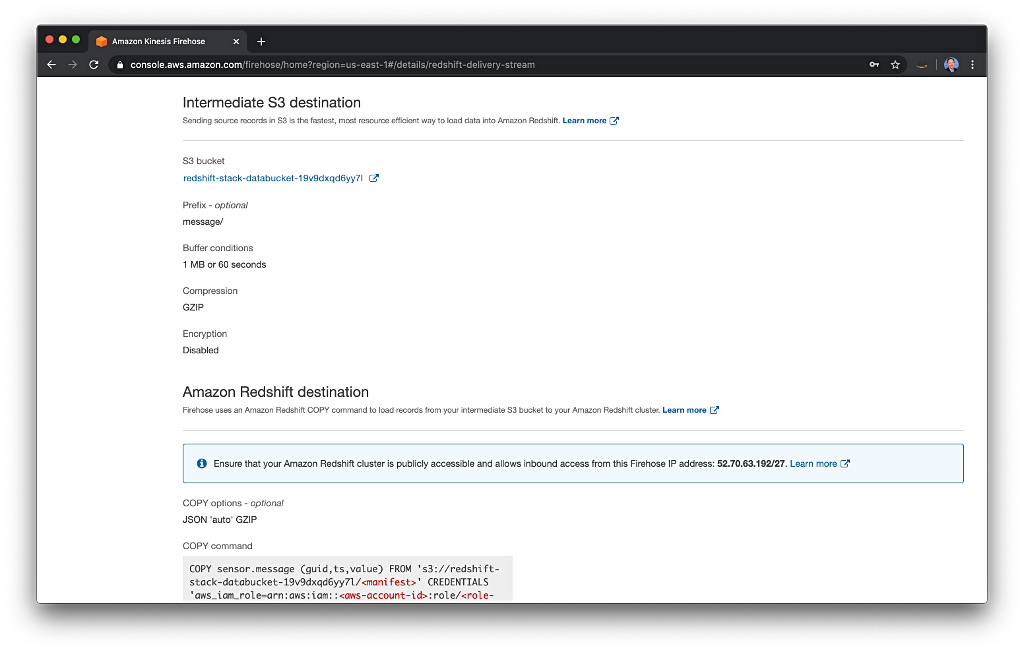
Note the COPY command, which is used to copy the messages from S3 to the message table in Amazon Redshift. Kinesis uses the IAM Role, ClusterPermissionsRole, created by CloudFormation, for credentials. We are using a Manifest to copy the data to Redshift from S3. According to Amazon, a Manifest ensures that the COPY command loads all of the required files, and only the required files, for a data load. The Manifests are automatically generated and managed by the Kinesis Firehose delivery stream.

Redshift Cluster

In the Amazon Redshift Console, you should see a new single-node Redshift cluster consisting of one Redshift dc2.large Dense Compute node type.

Note the new VPC, Subnet, and VPC Security Group created by CloudFormation. Also, observe that the Redshift cluster is publicly accessible from outside the new VPC.

Redshift Ingress Rules

The single-node Redshift cluster is assigned to an AWS Availability Zone in the US East (N. Virginia) us-east-1 AWS Region. The cluster is associated with a VPC Security Group. The Security Group contains three inbound rules, all for Redshift port 5439. The IP addresses associated with the three inbound rules provide access to the following: 1) a /27 CIDR block for Amazon QuickSight in us-east-1, a /27 CIDR block for Amazon Kinesis Firehose in us-east-1, and to you, a /32 CIDR block with your current IP address. If your IP address changes or you do not use the us-east-1 Region, you will need to change one or all of these IP addresses. The list of Kinesis Firehose IP addresses is here. The list of QuickSight IP addresses is here.

If you cannot connect to Redshift from your local SQL client, most often, your IP address has changed and is incorrect in the Security Group’s inbound rule.

Redshift SQL Client

You can choose to use the Redshift Query Editor to interact with Redshift or use a third-party SQL client for greater flexibility. To access the Redshift Query Editor, use the user credentials specified in the redshift.yml CloudFormation template.

There is a lot of useful functionality in the Redshift Console and within the Redshift Query Editor. However, a notable limitation of the Redshift Query Editor, in my opinion, is the inability to execute multiple SQL statements at the same time. Whereas, most SQL clients allow multiple SQL queries to be executed at the same time.

I prefer to use JetBrains PyCharm IDE. PyCharm has out-of-the-box integration with Redshift. Using PyCharm, I can edit the project’s Python, SQL, AWS CLI shell, and CloudFormation code, all from within PyCharm.

If you use any of the common SQL clients, you will need to set-up a JDBC (Java Database Connectivity) or ODBC (Open Database Connectivity) connection to Redshift. The ODBC and JDBC connection strings can be found in the Redshift cluster’s Properties tab or in the Outputs tab from the CloudFormation stack, redshift-stack.

You will also need the Redshift database username and password you included in the aws cloudformation create-stack AWS CLI command you executed previously. Below, we see PyCharm’s Project Data Sources window containing a new data source for the Redshift dev database.

Database Schema and Tables

When CloudFormation created the Redshift cluster, it also created a new database, dev. Using the Redshift Query Editor or your SQL client of choice, execute the following series of SQL commands to create a new database schema, sensor, and six tables in the sensor schema.

	— Create new schema in Redshift DB
	DROP SCHEMA IF EXISTS sensor CASCADE;
	CREATE SCHEMA sensor;
	SET search_path = sensor;

	— Create (6) tables in Redshift DB
	CREATE TABLE message — streaming data table
	(
	id BIGINT IDENTITY (1, 1), — message id
	guid VARCHAR(36) NOT NULL, — device guid
	ts BIGINT NOT NULL DISTKEY SORTKEY, — epoch in seconds
	temp NUMERIC(5, 2) NOT NULL, — temperature reading
	created TIMESTAMP DEFAULT ('now'::text)::timestamp with time zone — row created at
	);

	CREATE TABLE location — dimension table
	(
	id INTEGER NOT NULL DISTKEY SORTKEY, — location id
	long NUMERIC(10, 7) NOT NULL, — longitude
	lat NUMERIC(10, 7) NOT NULL, — latitude
	description VARCHAR(256) — location description
	);

	CREATE TABLE history — dimension table
	(
	id INTEGER NOT NULL DISTKEY SORTKEY, — history id
	serviced BIGINT NOT NULL, — service date
	action VARCHAR(20) NOT NULL, — INSTALLED, CALIBRATED, FIRMWARE UPGRADED, DECOMMISSIONED, OTHER
	technician_id INTEGER NOT NULL, — technician id
	notes VARCHAR(256) — notes
	);

	CREATE TABLE sensor — dimension table
	(
	id INTEGER NOT NULL DISTKEY SORTKEY, — sensor id
	guid VARCHAR(36) NOT NULL, — device guid
	mac VARCHAR(18) NOT NULL, — mac address
	sku VARCHAR(18) NOT NULL, — product sku
	upc VARCHAR(12) NOT NULL, — product upc
	active BOOLEAN DEFAULT TRUE, –active status
	notes VARCHAR(256) — notes

	);

	CREATE TABLE manufacturer — dimension table
	(
	id INTEGER NOT NULL DISTKEY SORTKEY, — manufacturer id
	name VARCHAR(100) NOT NULL, — company name
	website VARCHAR(100) NOT NULL, — company website
	notes VARCHAR(256) — notes
	);

	CREATE TABLE sensors — fact table
	(
	id BIGINT IDENTITY (1, 1) DISTKEY SORTKEY, — fact id
	sensor_id INTEGER NOT NULL, — sensor id
	manufacturer_id INTEGER NOT NULL, — manufacturer id
	location_id INTEGER NOT NULL, — location id
	history_id BIGINT NOT NULL, — history id
	message_guid VARCHAR(36) NOT NULL — sensor guid
	);

view raw

kinesis-redshift-schema-tables.sql

hosted with ❤ by GitHub

Star Schema

The tables represent denormalized data, taken from one or more relational database sources. The tables form a star schema. The star schema is widely used to develop data warehouses. The star schema consists of one or more fact tables referencing any number of dimension tables. The location, manufacturer, sensor, and history tables are dimension tables. The sensors table is a fact table.

In the diagram below, the foreign key relationships are virtual, not physical. The diagram was created using PyCharm’s schema visualization tool. Note the schema’s star shape. The message table is where the streaming IoT data will eventually be written. The message table is related to the sensors fact table through the common guid field.

Sample Data to S3

Next, copy the sample data, included in the project, to the S3 data bucket created with CloudFormation. Each CSV-formatted data file corresponds to one of the tables we previously created. Since the bucket name is semi-random, we can use the AWS CLI and jq to get the bucket name, then use it to perform the copy commands.

	# Get data bucket name
	DATA_BUCKET=$(aws cloudformation describe-stacks \
	–stack-name redshift-stack \
	\| jq -r '.Stacks[].Outputs[] \| select(.OutputKey == "DataBucket") \| .OutputValue')

	echo $DATA_BUCKET

	# Copy data
	aws s3 cp data/history.csv s3://${DATA_BUCKET}/history/history.csv
	aws s3 cp data/location.csv s3://${DATA_BUCKET}/location/location.csv
	aws s3 cp data/manufacturer.csv s3://${DATA_BUCKET}/manufacturer/manufacturer.csv
	aws s3 cp data/sensor.csv s3://${DATA_BUCKET}/sensor/sensor.csv
	aws s3 cp data/sensors.csv s3://${DATA_BUCKET}/sensors/sensors.csv

view raw

kinesis-redshift-copy-data.sh

hosted with ❤ by GitHub

The output from the AWS CLI should look similar to the following.

Sample Data to Redshift

Whereas a relational database, such as Amazon RDS is designed for online transaction processing (OLTP), Amazon Redshift is designed for online analytic processing (OLAP) and business intelligence applications. To write data to Redshift we typically use the COPY command versus frequent, individual INSERT statements, as with OLTP, which would be prohibitively slow. According to Amazon, the Redshift COPY command leverages the Amazon Redshift massively parallel processing (MPP) architecture to read and load data in parallel from files on Amazon S3, from a DynamoDB table, or from text output from one or more remote hosts.

In the following series of SQL statements, replace the placeholder, your_bucket_name, in five places with your S3 data bucket name. The bucket name will start with the prefix, redshift-stack-databucket. The bucket name can be found in the Outputs tab of the CloudFormation stack, redshift-stack. Next, replace the placeholder, cluster_permissions_role_arn, with the ARN (Amazon Resource Name) of the ClusterPermissionsRole. The ARN is formatted as follows, arn:aws:iam::your-account-id:role/ClusterPermissionsRole. The ARN can be found in the Outputs tab of the CloudFormation stack, redshift-stack.

Using the Redshift Query Editor or your SQL client of choice, execute the SQL statements to copy the sample data from S3 to each of the corresponding tables in the Redshift dev database. The TRUNCATE commands guarantee there is no previous sample data present in the tables.

	— MUST FIRST CHANGE your_bucket_name and cluster_permissions_role_arn

	— sensor schema
	SET search_path = sensor;

	— Copy sample data to tables from S3
	TRUNCATE TABLE history;
	COPY history (id, serviced, action, technician_id, notes)
	FROM 's3://your_bucket_name/history/'
	CREDENTIALS 'aws_iam_role=cluster_permissions_role_arn'
	CSV IGNOREHEADER 1;

	TRUNCATE TABLE location;
	COPY location (id, long, lat, description)
	FROM 's3://your_bucket_name/location/'
	CREDENTIALS 'aws_iam_role=cluster_permissions_role_arn'
	CSV IGNOREHEADER 1;

	TRUNCATE TABLE sensor;
	COPY sensor (id, guid, mac, sku, upc, active, notes)
	FROM 's3://your_bucket_name/sensor/'
	CREDENTIALS 'aws_iam_role=cluster_permissions_role_arn'
	CSV IGNOREHEADER 1;

	TRUNCATE TABLE manufacturer;
	COPY manufacturer (id, name, website, notes)
	FROM 's3://your_bucket_name/manufacturer/'
	CREDENTIALS 'aws_iam_role=cluster_permissions_role_arn'
	CSV IGNOREHEADER 1;

	TRUNCATE TABLE sensors;
	COPY sensors (sensor_id, manufacturer_id, location_id, history_id, message_guid)
	FROM 's3://your_bucket_name/sensors/'
	CREDENTIALS 'aws_iam_role=cluster_permissions_role_arn'
	CSV IGNOREHEADER 1;

	SELECT COUNT(*) FROM history; — 30
	SELECT COUNT(*) FROM location; — 6
	SELECT COUNT(*) FROM sensor; — 6
	SELECT COUNT(*) FROM manufacturer; –1
	SELECT COUNT(*) FROM sensors; — 30

view raw

kinesis-redshift-copy.sql

hosted with ❤ by GitHub

Database Views

Next, create four Redshift database Views. These views may be used to analyze the data in Redshift, and later, in Amazon QuickSight.

sensor_msg_detail: Returns aggregated sensor details, using the sensors fact table and all five dimension tables in a SQL Join.
sensor_msg_count: Returns the number of messages received by Redshift, for each sensor.
sensor_avg_temp: Returns the average temperature from each sensor, based on all the messages received from each sensor.
sensor_avg_temp_current: View is identical for the previous view but limited to the last 30 minutes.

Using the Redshift Query Editor or your SQL client of choice, execute the following series of SQL statements.

	— sensor schema
	SET search_path = sensor;

	— View 1: Sensor details
	DROP VIEW IF EXISTS sensor_msg_detail;
	CREATE OR REPLACE VIEW sensor_msg_detail AS
	SELECT ('1970-01-01'::date + e.ts * interval '1 second') AS recorded,
	e.temp,
	s.guid,
	s.sku,
	s.mac,
	l.lat,
	l.long,
	l.description AS location,
	('1970-01-01'::date + h.serviced * interval '1 second') AS installed,
	e.created AS redshift
	FROM sensors f
	INNER JOIN sensor s ON (f.sensor_id = s.id)
	INNER JOIN history h ON (f.history_id = h.id)
	INNER JOIN location l ON (f.location_id = l.id)
	INNER JOIN manufacturer m ON (f.manufacturer_id = m.id)
	INNER JOIN message e ON (f.message_guid = e.guid)
	WHERE s.active IS TRUE
	AND h.action = 'INSTALLED'
	ORDER BY f.id;

	— View 2: Message count per sensor
	DROP VIEW IF EXISTS sensor_msg_count;
	CREATE OR REPLACE VIEW sensor_msg_count AS
	SELECT count(e.temp) AS msg_count,
	s.guid,
	l.lat,
	l.long,
	l.description AS location
	FROM sensors f
	INNER JOIN sensor s ON (f.sensor_id = s.id)
	INNER JOIN history h ON (f.history_id = h.id)
	INNER JOIN location l ON (f.location_id = l.id)
	INNER JOIN message e ON (f.message_guid = e.guid)
	WHERE s.active IS TRUE
	AND h.action = 'INSTALLED'
	GROUP BY s.guid, l.description, l.lat, l.long
	ORDER BY msg_count, s.guid;

	— View 3: Average temperature per sensor (all data)
	DROP VIEW IF EXISTS sensor_avg_temp;
	CREATE OR REPLACE VIEW sensor_avg_temp AS
	SELECT avg(e.temp) AS avg_temp,
	count(s.guid) AS msg_count,
	s.guid,
	l.lat,
	l.long,
	l.description AS location
	FROM sensors f
	INNER JOIN sensor s ON (f.sensor_id = s.id)
	INNER JOIN history h ON (f.history_id = h.id)
	INNER JOIN location l ON (f.location_id = l.id)
	INNER JOIN message e ON (f.message_guid = e.guid)
	WHERE s.active IS TRUE
	AND h.action = 'INSTALLED'
	GROUP BY s.guid, l.description, l.lat, l.long
	ORDER BY avg_temp, s.guid;

	— View 4: Average temperature per sensor (last 30 minutes)
	DROP VIEW IF EXISTS sensor_avg_temp_current;
	CREATE OR REPLACE VIEW sensor_avg_temp_current AS
	SELECT avg(e.temp) AS avg_temp,
	count(s.guid) AS msg_count,
	s.guid,
	l.lat,
	l.long,
	l.description AS location
	FROM sensors f
	INNER JOIN sensor s ON (f.sensor_id = s.id)
	INNER JOIN history h ON (f.history_id = h.id)
	INNER JOIN location l ON (f.location_id = l.id)
	INNER JOIN (SELECT ('1970-01-01'::date + ts * interval '1 second') AS recorded_time,
	guid,
	temp
	FROM message
	WHERE DATEDIFF(minute, recorded_time, GETDATE()) <= 30) e ON (f.message_guid = e.guid)
	WHERE s.active IS TRUE
	AND h.action = 'INSTALLED'
	GROUP BY s.guid, l.description, l.lat, l.long
	ORDER BY avg_temp, s.guid;

view raw

kinesis-redshift-views.sql

hosted with ❤ by GitHub

At this point, you should have a total of six tables and four views in the sensor schema of the dev database in Redshift.

Test the System

With all the necessary AWS resources and Redshift database objects created and sample data in the Redshift database, we can test the system. The included Python script, kinesis_put_test_msg.py, will generate a single test message and send it to Kinesis Data Firehose. If everything is working, the message should be delivered from Kinesis Data Firehose to S3, then copied to Redshift, and appear in the message table.

Install the required Python packages and then execute the Python script.

	# Install required Python packages
	python3 -m pip install –user -r scripts/requirements.txt

	# Set default AWS Region for script
	export AWS_DEFAULT_REGION=us-east-1

	# Execute script in foreground
	python3 ./scripts/kinesis_put_test_msg.py

view raw

kinesis-redshift-test-msg.sh

hosted with ❤ by GitHub

Run the following SQL query to confirm the record is in the message table of the dev database. It will take at least one minute for the message to appear in Redshift.

SELECT COUNT(*) FROM message;

view raw

kinesis-redshift-test-query.sql

hosted with ❤ by GitHub

Once the message is confirmed to be present in the message table, delete the record by truncating the table.

TRUNCATE TABLE message;

view raw

kinesis-redshift-trun-msg.sql

hosted with ❤ by GitHub

Streaming Data

Assuming the test message worked, we can proceed with simulating the streaming IoT sensor data. The included Python script, kinesis_put_streaming_data.py, creates six concurrent threads, representing six temperature sensors.

	#!/usr/bin/env python3

	# Simulated multiple streaming time-series iot sensor data
	# Author: Gary A. Stafford
	# Date: Revised October 2020

	import json
	import random
	from datetime import datetime

	import boto3
	import time as tm
	import numpy as np
	import threading

	STREAM_NAME = 'redshift-delivery-stream'

	client = boto3.client('firehose')


	class MyThread(threading.Thread):
	def __init__(self, thread_id, sensor_guid, temp_max):
	threading.Thread.__init__(self)
	self.thread_id = thread_id
	self.sensor_id = sensor_guid
	self.temp_max = temp_max

	def run(self):
	print("Starting Thread: " + str(self.thread_id))
	self.create_data()
	print("Exiting Thread: " + str(self.thread_id))

	def create_data(self):
	start = 0
	stop = 20
	step = 0.1 # step size (e.g 0 to 20, step .1 = 200 steps in cycle)
	repeat = 2 # how many times to repeat cycle
	freq = 60 # frequency of temperature reading in seconds
	max_range = int(stop * (1 / step))
	time = np.arange(start, stop, step)
	amplitude = np.sin(time)
	for x in range(0, repeat):
	for y in range(0, max_range):
	temperature = round((((amplitude[y] + 1.0) * self.temp_max) + random.uniform(-5, 5)) + 60, 2)
	payload = {
	'guid': self.sensor_id,
	'ts': int(datetime.now().strftime('%s')),
	'temp': temperature
	}

	print(json.dumps(payload))

	self.send_to_kinesis(payload)

	tm.sleep(freq)

	@staticmethod
	def send_to_kinesis(payload):
	_ = client.put_record(
	DeliveryStreamName=STREAM_NAME,
	Record={
	'Data': json.dumps(payload)
	}
	)


	def main():
	sensor_guids = [
	"03e39872-e105-4be4-83c0-9ade818465dc",
	"fa565921-fddd-4bfb-a7fd-d617f816df4b",
	"d120422d-5789-435d-9dc6-73d8489b04c2",
	"93238559-4d55-4b2a-bdcb-6aa3be0f3908",
	"dbc05806-6872-4f0a-aca2-f794cc39bd9b",
	"f9ade639-f936-4954-aa5a-1f2ed86c9bcf"
	]
	timeout = 300 # arbitrarily offset the start of threads (60 / 5 = 12)

	# Create new threads
	thread1 = MyThread(1, sensor_guids[0], 25)
	thread2 = MyThread(2, sensor_guids[1], 10)
	thread3 = MyThread(3, sensor_guids[2], 7)
	thread4 = MyThread(4, sensor_guids[3], 30)
	thread5 = MyThread(5, sensor_guids[4], 5)
	thread6 = MyThread(6, sensor_guids[5], 12)

	# Start new threads
	thread1.start()
	tm.sleep(timeout * 1)
	thread2.start()
	tm.sleep(timeout * 2)
	thread3.start()
	tm.sleep(timeout * 1)
	thread4.start()
	tm.sleep(timeout * 3)
	thread5.start()
	tm.sleep(timeout * 2)
	thread6.start()

	# Wait for threads to terminate
	thread1.join()
	thread2.join()
	thread3.join()
	thread4.join()
	thread5.join()
	thread6.join()
	print("Exiting Main Thread")


	if __name__ == '__main__':
	main()

view raw

kinesis_put_streaming_data.py

hosted with ❤ by GitHub

The simulated data uses an algorithm that follows an oscillating sine wave or sinusoid, representing rising and falling temperatures. In the script, I have configured each thread to start with an arbitrary offset to add some randomness to the simulated data.

The variables within the script can be adjusted to shorten or lengthen the time it takes to stream the simulated data. By default, each of the six threads creates 400 messages per sensor, in one-minute increments. Including the offset start of each proceeding thread, the total runtime of the script is about 7.5 hours to generate 2,400 simulated IoT sensor temperature readings and push to Kinesis Data Firehose. Make sure you can guarantee you will maintain a connection to the Internet for the entire runtime of the script. I normally run the script in the background, from a small EC2 instance.

To use the Python script, execute either of the two following commands. Using the first command will run the script in the foreground. Using the second command will run the script in the background.

	# Install required Python packages
	python3 -m pip install –user -r scripts/requirements.txt

	# Set default AWS Region for script
	export AWS_DEFAULT_REGION=us-east-1

	# Option #1: Execute script in foreground
	python3 ./scripts/kinesis_put_streaming_data.py

	# Option #2: execute script in background
	nohup python3 -u ./scripts/kinesis_put_streaming_data.py > output.log 2>&1 </dev/null &

	# Check that the process is running
	ps -aux \| grep 'python3 -u ./scripts/kinesis_put_streaming_data.py'

	# Wait 1-2 minutes, then check output to confirm script is working
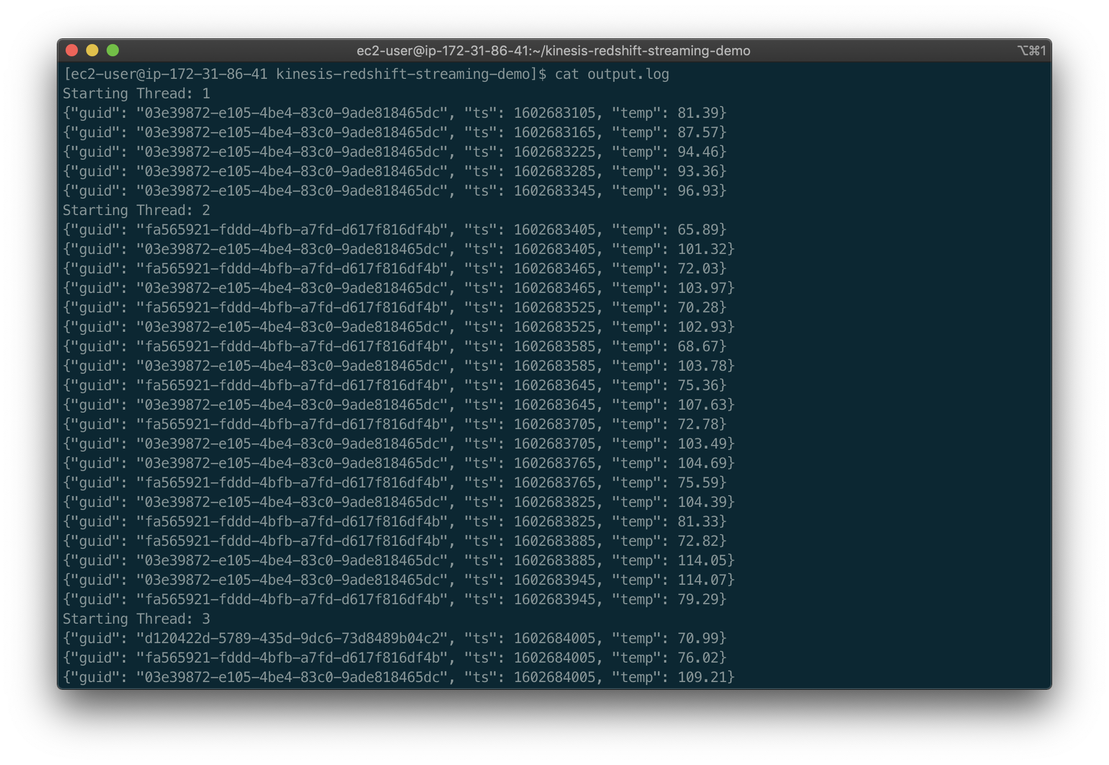
	cat output.log

view raw

kinesis-redshift-streaming-data.sh

hosted with ❤ by GitHub

Viewing the output.log file, you should see messages being generated on each thread and sent to Kinesis Data Firehose. Each message contains the GUID of the sensor, a timestamp, and a temperature reading.

Screen Shot 2020-10-14 at 10.00.37 AM

The messages are sent to Kinesis Data Firehose, which in turn writes the messages to S3. The messages are written in JSON format using GZIP compression. Below, we see an example of the GZIP compressed JSON files in S3. The JSON files are partitioned by year, month, day, and hour.

Confirm Data Streaming to Redshift

From the Amazon Kinesis Firehose Console Metrics tab, you should see incoming messages flowing to S3 and on to Redshift.

Executing the following SQL query should show an increasing number of messages.

SELECT COUNT(*) FROM message;

view raw

kinesis-redshift-test-query.sql

hosted with ❤ by GitHub

How Near Real-time?

Earlier, we saw how the Amazon Kinesis Data Firehose delivery stream was configured to buffer data at the rate of 1 MB or 60 seconds. Whenever the buffer of incoming messages is greater than 1 MB or the time exceeds 60 seconds, the messages are written to S3. Each record in the message table has two timestamps. The first timestamp, ts, is when the temperature reading was recorded. The second timestamp, created, is when the message was written to Redshift, using the COPY command. We can calculate the delta in seconds between the two timestamps using the following SQL query in Redshift.

	SELECT ('1970-01-01'::date + ts * interval '1 second') AS recorded_time,
	created AS redshift_time,
	DATEDIFF(seconds, recorded_time, redshift_time) AS diff_seconds
	FROM message
	ORDER BY diff_seconds;

view raw

kinesis-redshift-latency.sql

hosted with ❤ by GitHub

Using the results of the Redshift query, we can visualize the results in Amazon QuickSight. In my own tests, we see that for 2,400 messages, over approximately 7.5 hours, the minimum delay was 1 second, and a maximum delay was 64 seconds. Hence, near real-time, in this case, is about one minute or less, with an average latency of roughly 30 seconds.

Analyzing the Data with Redshift

I suggest waiting at least thirty minutes for a significant number of messages copied into Redshift. With the data streaming into Redshift, execute each of the database views we created earlier. You should see the streaming message data, joined to the existing static data in Redshift. As data continues to stream into Redshift, the views will display different results based on the current message table contents.

Here, we see the first ten results of the sensor_msg_detail view.

recorded	temp	guid	sku	mac	lat	long	location	installed	redshift
2020-03-04 03:31:59.000000	105.56	03e39872-e105-4be4-83c0-9ade818465dc	PR49-24A	8e:fa:46:09:14:b2	37.7068476	-122.4191599	Research Lab #2203	2018-01-31 12:00:00.000000	2020-03-04 03:33:01.580147
2020-03-04 03:29:59.000000	95.93	03e39872-e105-4be4-83c0-9ade818465dc	PR49-24A	8e:fa:46:09:14:b2	37.7068476	-122.4191599	Research Lab #2203	2018-01-31 12:00:00.000000	2020-03-04 03:31:01.388887
2020-03-04 03:26:58.000000	91.93	03e39872-e105-4be4-83c0-9ade818465dc	PR49-24A	8e:fa:46:09:14:b2	37.7068476	-122.4191599	Research Lab #2203	2018-01-31 12:00:00.000000	2020-03-04 03:28:01.099796
2020-03-04 03:25:58.000000	88.70	03e39872-e105-4be4-83c0-9ade818465dc	PR49-24A	8e:fa:46:09:14:b2	37.7068476	-122.4191599	Research Lab #2203	2018-01-31 12:00:00.000000	2020-03-04 03:26:00.196113
2020-03-04 03:22:58.000000	87.65	03e39872-e105-4be4-83c0-9ade818465dc	PR49-24A	8e:fa:46:09:14:b2	37.7068476	-122.4191599	Research Lab #2203	2018-01-31 12:00:00.000000	2020-03-04 03:23:01.558514
2020-03-04 03:20:58.000000	77.35	03e39872-e105-4be4-83c0-9ade818465dc	PR49-24A	8e:fa:46:09:14:b2	37.7068476	-122.4191599	Research Lab #2203	2018-01-31 12:00:00.000000	2020-03-04 03:21:00.691347
2020-03-04 03:16:57.000000	71.84	03e39872-e105-4be4-83c0-9ade818465dc	PR49-24A	8e:fa:46:09:14:b2	37.7068476	-122.4191599	Research Lab #2203	2018-01-31 12:00:00.000000	2020-03-04 03:17:59.307510
2020-03-04 03:15:57.000000	72.35	03e39872-e105-4be4-83c0-9ade818465dc	PR49-24A	8e:fa:46:09:14:b2	37.7068476	-122.4191599	Research Lab #2203	2018-01-31 12:00:00.000000	2020-03-04 03:15:59.813656
2020-03-04 03:14:57.000000	67.95	03e39872-e105-4be4-83c0-9ade818465dc	PR49-24A	8e:fa:46:09:14:b2	37.7068476	-122.4191599	Research Lab #2203	2018-01-31 12:00:00.000000	2020-03-04 03:15:59.813656

view raw

kinesis-redshift-sample-data.csv

hosted with ❤ by GitHub

Next, we see the results of the sensor_avg_temp view.

avg_temp	guid	lat	long	location
65.25	dbc05806-6872-4f0a-aca2-f794cc39bd9b	37.7066541	-122.4181399	Wafer Inspection Lab #0210A
67.23	d120422d-5789-435d-9dc6-73d8489b04c2	37.7072686	-122.4187016	Zone 4 Wafer Processing Area B3
70.23	fa565921-fddd-4bfb-a7fd-d617f816df4b	37.7071763	-122.4190397	Research Lab #2209
72.22	f9ade639-f936-4954-aa5a-1f2ed86c9bcf	37.7067618	-122.4186191	Wafer Inspection Lab #0211C
85.48	03e39872-e105-4be4-83c0-9ade818465dc	37.7068476	-122.4191599	Research Lab #2203
90.69	93238559-4d55-4b2a-bdcb-6aa3be0f3908	37.7070334	-122.4184393	Zone 2 Semiconductor Assembly Area A2

view raw

kinesis-redshift-sample-data-2.csv

hosted with ❤ by GitHub

Amazon QuickSight

In a recent post, Getting Started with Data Analysis on AWS using AWS Glue, Amazon Athena, and QuickSight: Part 2, I detailed getting started with Amazon QuickSight. In this post, I will assume you are familiar with QuickSight.

Amazon recently added a full set of aws quicksight APIs for interacting with QuickSight. Though, for this part of the demonstration, we will be working directly in the Amazon QuickSight Console, as opposed to the AWS CLI, AWS CDK, or CloudFormation.

Redshift Data Sets

To visualize the data from Amazon Redshift, we start by creating Data Sets in QuickSight. QuickSight supports a large number of data sources for creating data sets. We will use the Redshift data source. If you recall, we added an inbound rule for QuickSight, allowing us to connect to our Redshift cluster in us-east-1.

We will select the sensor schema, which is where the tables and views for this demonstration are located.

We can choose any of the tables or views in the Redshift dev database that we want to use for visualization.

Below, we see examples of two new data sets, shown in the QuickSight Data Prep Console. Note how QuickSight automatically recognizes field types, including dates, latitude, and longitude.

Visualizations

Using the data sets, QuickSight allows us to create a wide number of rich visualizations. Below, we see the simulated time-series data from the six temperature sensors.

Next, we see an example of QuickSight’s ability to show geospatial data. The Map shows the location of each sensor and the average temperature recorded by that sensor.

Cleaning Up

To remove the resources created for this post, use the following series of AWS CLI commands.

	# Get data bucket name
	DATA_BUCKET=$(aws cloudformation describe-stacks \
	–stack-name redshift-stack \
	\| jq -r '.Stacks[].Outputs[] \| select(.OutputKey == "DataBucket") \| .OutputValue')

	echo ${DATA_BUCKET}

	# Get log bucket name
	LOG_BUCKET=$(aws cloudformation describe-stacks \
	–stack-name redshift-stack \
	\| jq -r '.Stacks[].Outputs[] \| select(.OutputKey == "LogBucket") \| .OutputValue')

	echo ${LOG_BUCKET}

	# Delete demonstration resources
	python3 ./scripts/delete_buckets.py

	aws cloudformation delete-stack –stack-name kinesis-firehose-stack

	# Wait for first stack to be deleted
	aws cloudformation delete-stack –stack-name redshift-stack

view raw

kinesis-redshift-cleanup.sh

hosted with ❤ by GitHub

Conclusion

In this brief post, we have learned how streaming data can be analyzed in near real-time, in Amazon Redshift, using Amazon Kinesis Data Firehose. Further, we explored how the results of those analyses can be visualized in Amazon QuickSight. For customers that depend on a data warehouse for data analytics, but who also have streaming data sources, the use of Amazon Kinesis Data Firehose or Amazon Redshift Spectrum is an excellent choice.

This blog represents my own viewpoints and not of my employer, Amazon Web Services.

Amazon, AWS, Data Warehouse, IoT, Kinesis Data Firehose, QuickSight, RedShift, Streaming data

1 Comment