Posts Tagged Apache Superset
Exploring Popular Open-source Stream Processing Technologies: Part 2 of 2
Posted by Gary A. Stafford in Analytics, Big Data, Java Development, Python, Software Development, SQL on September 26, 2022
A brief demonstration of Apache Spark Structured Streaming, Apache Kafka Streams, Apache Flink, and Apache Pinot with Apache Superset
Introduction
According to TechTarget, “Stream processing is a data management technique that involves ingesting a continuous data stream to quickly analyze, filter, transform or enhance the data in real-time. Once processed, the data is passed off to an application, data store, or another stream processing engine.” Confluent, a fully-managed Apache Kafka market leader, defines stream processing as “a software paradigm that ingests, processes, and manages continuous streams of data while they’re still in motion.”
This two-part post series and forthcoming video explore four popular open-source software (OSS) stream processing projects: Apache Spark Structured Streaming, Apache Kafka Streams, Apache Flink, and Apache Pinot.

This post uses the open-source projects, making it easier to follow along with the demonstration and keeping costs to a minimum. However, you could easily substitute the open-source projects for your preferred SaaS, CSP, or COSS service offerings.
Part Two
We will continue our exploration in part two of this two-part post, covering Apache Flink and Apache Pinot. In addition, we will incorporate Apache Superset into the demonstration to visualize the real-time results of our stream processing pipelines as a dashboard.
Demonstration #3: Apache Flink
In the third demonstration of four, we will examine Apache Flink. For this part of the post, we will also use the third of the three GitHub repository projects, flink-kafka-demo. The project contains a Flink application written in Java, which performs stream processing, incremental aggregation, and multi-stream joins.

New Streaming Stack
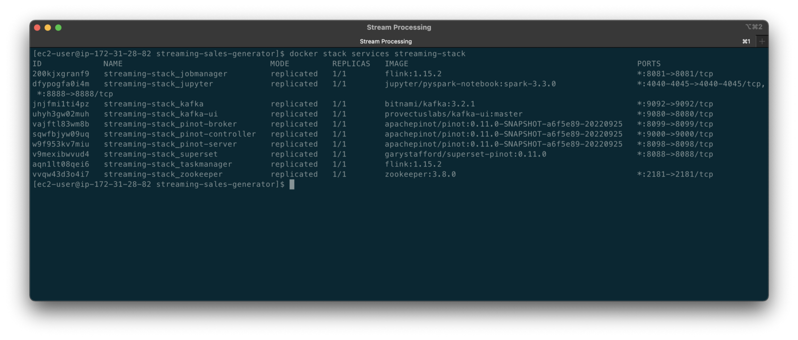
To get started, we need to replace the first streaming Docker Swarm stack, deployed in part one, with the second streaming Docker Swarm stack. The second stack contains Apache Kafka, Apache Zookeeper, Apache Flink, Apache Pinot, Apache Superset, UI for Apache Kafka, and Project Jupyter (JupyterLab).
https://programmaticponderings.wordpress.com/media/601efca17604c3a467a4200e93d7d3ff
The stack will take a few minutes to deploy fully. When complete, there should be ten containers running in the stack.
Flink Application
The Flink application has two entry classes. The first class, RunningTotals, performs an identical aggregation function as the previous KStreams demo.
The second class, JoinStreams, joins the stream of data from the demo.purchases topic and the demo.products topic, processing and combining them, in real-time, into an enriched transaction and publishing the results to a new topic, demo.purchases.enriched.
The resulting enriched purchases messages look similar to the following:
Running the Flink Job
To run the Flink application, we must first compile it into an uber JAR.
We can copy the JAR into the Flink container or upload it through the Apache Flink Dashboard, a browser-based UI. For this demonstration, we will upload it through the Apache Flink Dashboard, accessible on port 8081.
The project’s build.gradle file has preset the Main class (Flink’s Entry class) to org.example.JoinStreams. Optionally, to run the Running Totals demo, we could change the build.gradle file and recompile, or simply change Flink’s Entry class to org.example.RunningTotals.

Before running the Flink job, restart the sales generator in the background (nohup python3 ./producer.py &) to generate a new stream of data. Then start the Flink job.

To confirm the Flink application is running, we can check the contents of the new demo.purchases.enriched topic using the Kafka CLI.

Alternatively, you can use the UI for Apache Kafka, accessible on port 9080.

Demonstration #4: Apache Pinot
In the fourth and final demonstration, we will explore Apache Pinot. First, we will query the unbounded data streams from Apache Kafka, generated by both the sales generator and the Apache Flink application, using SQL. Then, we build a real-time dashboard in Apache Superset, with Apache Pinot as our datasource.

Creating Tables
According to the Apache Pinot documentation, “a table is a logical abstraction that represents a collection of related data. It is composed of columns and rows (known as documents in Pinot).” There are three types of Pinot tables: Offline, Realtime, and Hybrid. For this demonstration, we will create three Realtime tables. Realtime tables ingest data from streams — in our case, Kafka — and build segments from the consumed data. Further, according to the documentation, “each table in Pinot is associated with a Schema. A schema defines what fields are present in the table along with the data types. The schema is stored in Zookeeper, along with the table configuration.”
Below, we see the schema and config for one of the three Realtime tables, purchasesEnriched. Note how the columns are divided into three categories: Dimension, Metric, and DateTime.
To begin, copy the three Pinot Realtime table schemas and configurations from the streaming-sales-generator GitHub project into the Apache Pinot Controller container. Next, use a docker exec command to call the Pinot Command Line Interface’s (CLI) AddTable command to create the three tables: products, purchases, and purchasesEnriched.
To confirm the three tables were created correctly, use the Apache Pinot Data Explorer accessible on port 9000. Use the Tables tab in the Cluster Manager.

We can further inspect and edit the table’s config and schema from the Tables tab in the Cluster Manager.

The three tables are configured to read the unbounded stream of data from the corresponding Kafka topics: demo.products, demo.purchases, and demo.purchases.enriched.
Querying with Pinot
We can use Pinot’s Query Console to query the Realtime tables using SQL. According to the documentation, “Pinot provides a SQL interface for querying. It uses the [Apache] Calcite SQL parser to parse queries and uses MYSQL_ANSI dialect.”

With the generator still running, re-query the purchases table in the Query Console (select count(*) from purchases). You should notice the document count increasing each time you re-run the query since new messages are published to the demo.purchases topic by the sales generator.
If you do not observe the count increasing, ensure the sales generator and Flink enrichment job are running.

Table Joins?
It might seem logical to want to replicate the same multi-stream join we performed with Apache Flink in part three of the demonstration on the demo.products and demo.purchases topics. Further, we might presume to join the products and purchases realtime tables by writing a SQL statement in Pinot’s Query Console. However, according to the documentation, at the time of this post, version 0.11.0 of Pinot did not [currently] support joins or nested subqueries.
This current join limitation is why we created the Realtime table, purchasesEnriched, allowing us to query Flink’s real-time results in the demo.purchases.enriched topic. We will use both Flink and Pinot as part of our stream processing pipeline, taking advantage of each tool’s individual strengths and capabilities.
Note, according to the documentation for the latest release of Pinot on the main branch, “the latest Pinot multi-stage supports inner join, left-outer, semi-join, and nested queries out of the box. It is optimized for in-memory process and latency.” For more information on joins as part of Pinot’s new multi-stage query execution engine, read the documentation, Multi-Stage Query Engine.

demo.purchases.enriched topic in real-timeAggregations
We can perform real-time aggregations using Pinot’s rich SQL query interface. For example, like previously with Spark and Flink, we can calculate running totals for the number of items sold and the total sales for each product in real time.

We can do the same with the purchasesEnriched table, which will use the continuous stream of enriched transaction data from our Apache Flink application. With the purchasesEnriched table, we can add the product name and product category for richer results. Each time we run the query, we get real-time results based on the running sales generator and Flink enrichment job.

Query Options and Indexing
Note the reference to the Star-Tree index at the start of the SQL query shown above. Pinot provides several query options, including useStarTree (true by default).
Multiple indexing techniques are available in Pinot, including Forward Index, Inverted Index, Star-tree Index, Bloom Filter, and Range Index, among others. Each has advantages in different query scenarios. According to the documentation, by default, Pinot creates a dictionary-encoded forward index for each column.
SQL Examples
Here are a few examples of SQL queries you can try in Pinot’s Query Console:
Troubleshooting Pinot
If have issues with creating the tables or querying the real-time data, you can start by reviewing the Apache Pinot logs:
Real-time Dashboards with Apache Superset
To display the real-time stream of data produced results of our Apache Flink stream processing job and made queriable by Apache Pinot, we can use Apache Superset. Superset positions itself as “a modern data exploration and visualization platform.” Superset allows users “to explore and visualize their data, from simple line charts to highly detailed geospatial charts.”
According to the documentation, “Superset requires a Python DB-API database driver and a SQLAlchemy dialect to be installed for each datastore you want to connect to.” In the case of Apache Pinot, we can use pinotdb as the Python DB-API and SQLAlchemy dialect for Pinot. Since the existing Superset Docker container does not have pinotdb installed, I have built and published a Docker Image with the driver and deployed it as part of the second streaming stack of containers.
First, we much configure the Superset container instance. These instructions are documented as part of the Superset Docker Image repository.
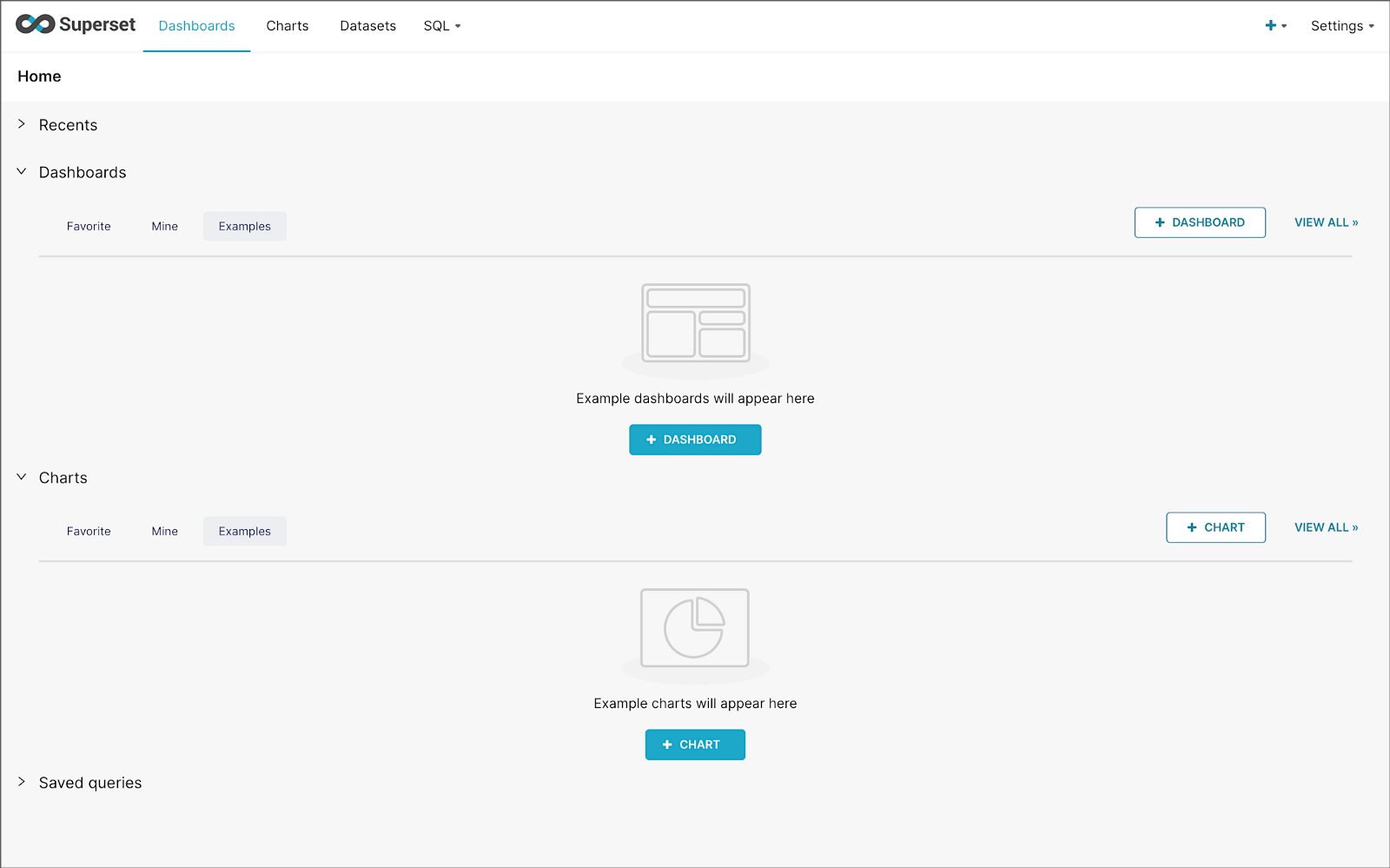
Once the configuration is complete, we can log into the Superset web-browser-based UI accessible on port 8088.
Pinot Database Connection and Dataset
Next, to connect to Pinot from Superset, we need to create a Database Connection and a Dataset.
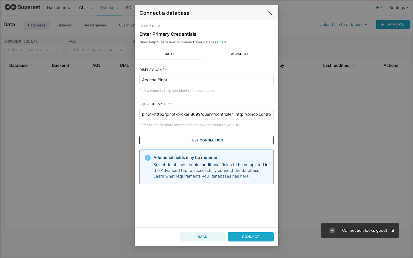
The SQLAlchemy URI is shown below. Input the URI, test your connection (‘Test Connection’), make sure it succeeds, then hit ‘Connect’.
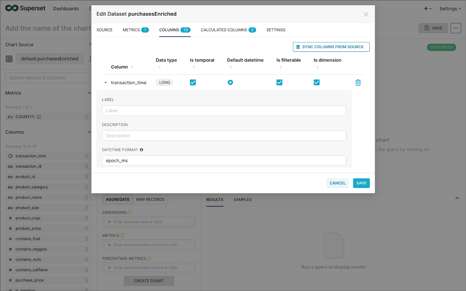
Next, create a Dataset that references the purchasesEnriched Pinot table.

purchasesEnriched Pinot tableModify the dataset’s transaction_time column. Check the is_temporal and Default datetime options. Lastly, define the DateTime format as epoch_ms.
transaction_time columnBuilding a Real-time Dashboard
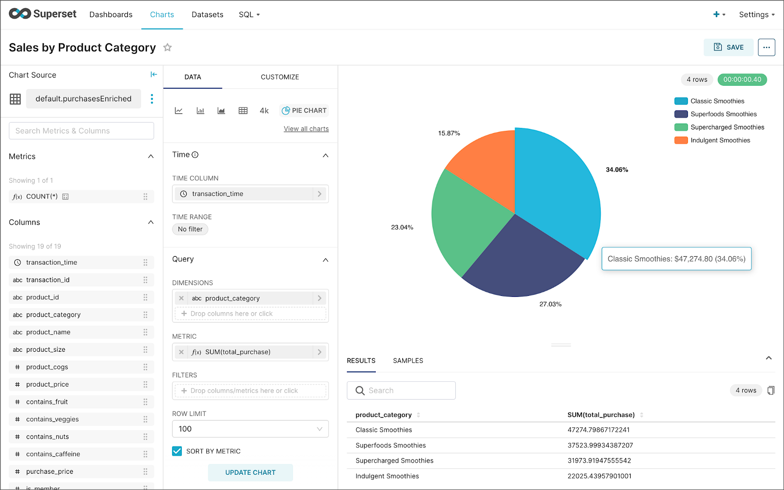
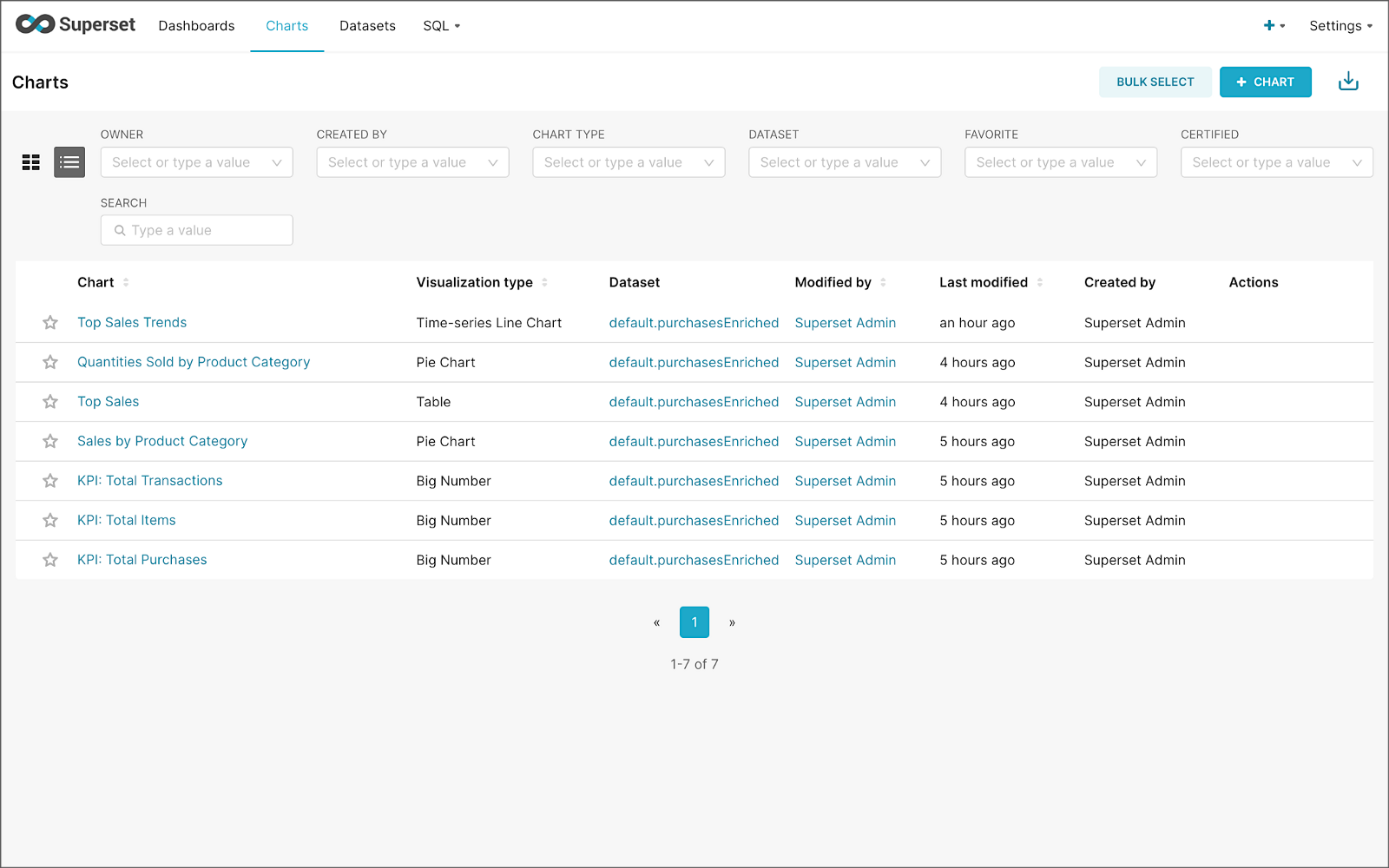
Using the new dataset, which connects Superset to the purchasesEnriched Pinot table, we can construct individual charts to be placed on a dashboard. Build a few charts to include on your dashboard.
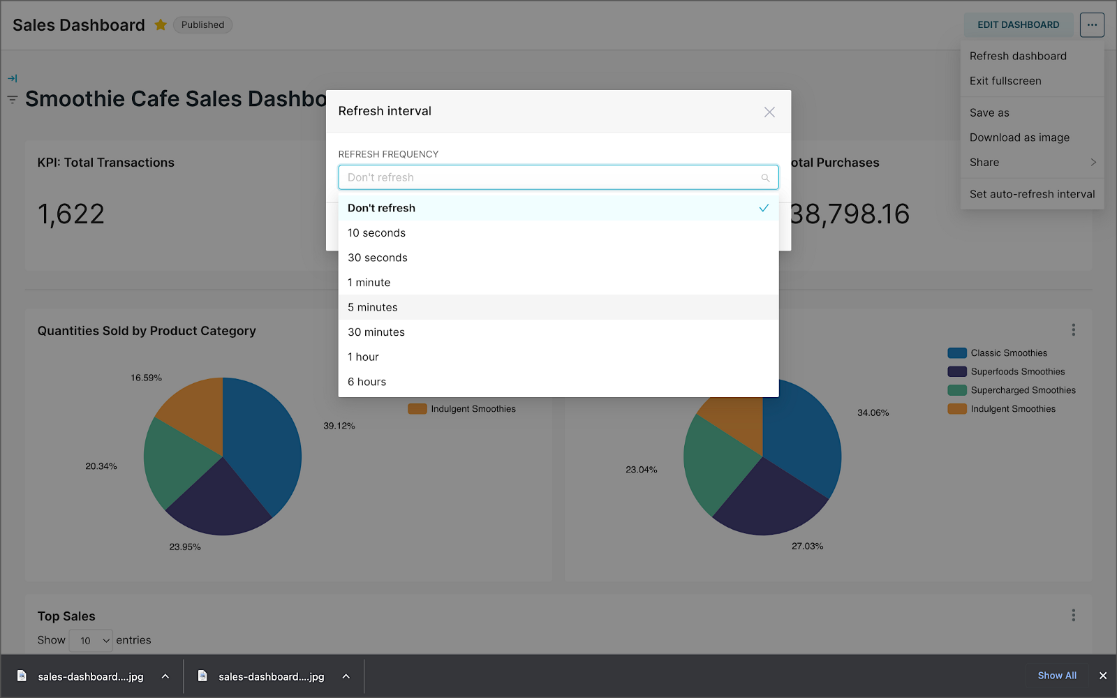
Create a new Superset dashboard and add the charts and other elements, such as headlines, dividers, and tabs.

We can apply a refresh interval to the dashboard to continuously query Pinot and visualize the results in near real-time.
Conclusion
In this two-part post series, we were introduced to stream processing. We explored four popular open-source stream processing projects: Apache Spark Structured Streaming, Apache Kafka Streams, Apache Flink, and Apache Pinot. Next, we learned how we could solve similar stream processing and streaming analytics challenges using different streaming technologies. Lastly, we saw how these technologies, such as Kafka, Flink, Pinot, and Superset, could be integrated to create effective stream processing pipelines.
This blog represents my viewpoints and not of my employer, Amazon Web Services (AWS). All product names, logos, and brands are the property of their respective owners. All diagrams and illustrations are the property of the author unless otherwise noted.
Exploring Popular Open-source Stream Processing Technologies: Part 1 of 2
Posted by Gary A. Stafford in Analytics, Big Data, Java Development, Python, Software Development, SQL on September 24, 2022
A brief demonstration of Apache Spark Structured Streaming, Apache Kafka Streams, Apache Flink, and Apache Pinot with Apache Superset
Introduction
According to TechTarget, “Stream processing is a data management technique that involves ingesting a continuous data stream to quickly analyze, filter, transform or enhance the data in real-time. Once processed, the data is passed off to an application, data store, or another stream processing engine.” Confluent, a fully-managed Apache Kafka market leader, defines stream processing as “a software paradigm that ingests, processes, and manages continuous streams of data while they’re still in motion.”
Batch vs. Stream Processing
Again, according to Confluent, “Batch processing is when the processing and analysis happens on a set of data that have already been stored over a period of time.” A batch processing example might include daily retail sales data, which is aggregated and tabulated nightly after the stores close. Conversely, “streaming data processing happens as the data flows through a system. This results in analysis and reporting of events as it happens.” To use a similar example, instead of nightly batch processing, the streams of sales data are processed, aggregated, and analyzed continuously throughout the day — sales volume, buying trends, inventory levels, and marketing program performance are tracked in real time.
Bounded vs. Unbounded Data
According to Packt Publishing’s book, Learning Apache Apex, “bounded data is finite; it has a beginning and an end. Unbounded data is an ever-growing, essentially infinite data set.” Batch processing is typically performed on bounded data, whereas stream processing is most often performed on unbounded data.
Stream Processing Technologies
There are many technologies available to perform stream processing. These include proprietary custom software, commercial off-the-shelf (COTS) software, fully-managed service offerings from Software as a Service (or SaaS) providers, Cloud Solution Providers (CSP), Commercial Open Source Software (COSS) companies, and popular open-source projects from the Apache Software Foundation and Linux Foundation.
The following two-part post and forthcoming video will explore four popular open-source software (OSS) stream processing projects, including Apache Spark Structured Streaming, Apache Kafka Streams, Apache Flink, and Apache Pinot. Each of these projects has some equivalent SaaS, CSP, and COSS offerings.
This post uses the open-source projects, making it easier to follow along with the demonstration and keeping costs to a minimum. However, you could easily substitute the open-source projects for your preferred SaaS, CSP, or COSS service offerings.
Apache Spark Structured Streaming
According to the Apache Spark documentation, “Structured Streaming is a scalable and fault-tolerant stream processing engine built on the Spark SQL engine. You can express your streaming computation the same way you would express a batch computation on static data.” Further, “Structured Streaming queries are processed using a micro-batch processing engine, which processes data streams as a series of small batch jobs thereby achieving end-to-end latencies as low as 100 milliseconds and exactly-once fault-tolerance guarantees.” In the post, we will examine both batch and stream processing using a series of Apache Spark Structured Streaming jobs written in PySpark.

Apache Kafka Streams
According to the Apache Kafka documentation, “Kafka Streams [aka KStreams] is a client library for building applications and microservices, where the input and output data are stored in Kafka clusters. It combines the simplicity of writing and deploying standard Java and Scala applications on the client side with the benefits of Kafka’s server-side cluster technology.” In the post, we will examine a KStreams application written in Java that performs stream processing and incremental aggregation.

Apache Flink
According to the Apache Flink documentation, “Apache Flink is a framework and distributed processing engine for stateful computations over unbounded and bounded data streams. Flink has been designed to run in all common cluster environments, perform computations at in-memory speed and at any scale.” Further, “Apache Flink excels at processing unbounded and bounded data sets. Precise control of time and state enables Flink’s runtime to run any kind of application on unbounded streams. Bounded streams are internally processed by algorithms and data structures that are specifically designed for fixed-sized data sets, yielding excellent performance.” In the post, we will examine a Flink application written in Java, which performs stream processing, incremental aggregation, and multi-stream joins.

Apache Pinot
According to Apache Pinot’s documentation, “Pinot is a real-time distributed OLAP datastore, purpose-built to provide ultra-low-latency analytics, even at extremely high throughput. It can ingest directly from streaming data sources — such as Apache Kafka and Amazon Kinesis — and make the events available for querying instantly. It can also ingest from batch data sources such as Hadoop HDFS, Amazon S3, Azure ADLS, and Google Cloud Storage.” In the post, we will query the unbounded data streams from Apache Kafka, generated by Apache Flink, using SQL.

Streaming Data Source
We must first find a good unbounded data source to explore or demonstrate these streaming technologies. Ideally, the streaming data source should be complex enough to allow multiple types of analyses and visualize different aspects with Business Intelligence (BI) and dashboarding tools. Additionally, the streaming data source should possess a degree of consistency and predictability while displaying a reasonable level of variability and randomness.
To this end, we will use the open-source Streaming Synthetic Sales Data Generator project, which I have developed and made available on GitHub. This project’s highly-configurable, Python-based, synthetic data generator generates an unbounded stream of product listings, sales transactions, and inventory restocking activities to a series of Apache Kafka topics.

Source Code
All the source code demonstrated in this post is open source and available on GitHub. There are three separate GitHub projects:
Docker
To make it easier to follow along with the demonstration, we will use Docker Swarm to provision the streaming tools. Alternatively, you could use Kubernetes (e.g., creating a Helm chart) or your preferred CSP or SaaS managed services. Nothing in this demonstration requires you to use a paid service.
The two Docker Swarm stacks are located in the Streaming Synthetic Sales Data Generator project:
- Streaming Stack — Part 1: Apache Kafka, Apache Zookeeper, Apache Spark, UI for Apache Kafka, and the KStreams application
- Streaming Stack — Part 2: Apache Kafka, Apache Zookeeper, Apache Flink, Apache Pinot, Apache Superset, UI for Apache Kafka, and Project Jupyter (JupyterLab).*
* the Jupyter container can be used as an alternative to the Spark container for running PySpark jobs (follow the same steps as for Spark, below)
Demonstration #1: Apache Spark
In the first of four demonstrations, we will examine two Apache Spark Structured Streaming jobs, written in PySpark, demonstrating both batch processing (spark_batch_kafka.py) and stream processing (spark_streaming_kafka.py). We will read from a single stream of data from a Kafka topic, demo.purchases, and write to the console.

Deploying the Streaming Stack
To get started, deploy the first streaming Docker Swarm stack containing the Apache Kafka, Apache Zookeeper, Apache Spark, UI for Apache Kafka, and the KStreams application containers.
The stack will take a few minutes to deploy fully. When complete, there should be a total of six containers running in the stack.

Sales Generator
Before starting the streaming data generator, confirm or modify the configuration/configuration.ini. Three configuration items, in particular, will determine how long the streaming data generator runs and how much data it produces. We will set the timing of transaction events to be generated relatively rapidly for test purposes. We will also set the number of events high enough to give us time to explore the Spark jobs. Using the below settings, the generator should run for an average of approximately 50–60 minutes: (((5 sec + 2 sec)/2)*1000 transactions)/60 sec=~58 min on average. You can run the generator again if necessary or increase the number of transactions.
Start the streaming data generator as a background service:
The streaming data generator will start writing data to three Apache Kafka topics: demo.products, demo.purchases, and demo.inventories. We can view these topics and their messages by logging into the Apache Kafka container and using the Kafka CLI:
Below, we see a few sample messages from the demo.purchases topic:

demo.purchases topicAlternatively, you can use the UI for Apache Kafka, accessible on port 9080.

demo.purchases topic in the UI for Apache Kafka
demo.purchases topic using the UI for Apache KafkaPrepare Spark
Next, prepare the Spark container to run the Spark jobs:
Running the Spark Jobs
Next, copy the jobs from the project to the Spark container, then exec back into the container:
Batch Processing with Spark
The first Spark job, spark_batch_kafka.py, aggregates the number of items sold and the total sales for each product, based on existing messages consumed from the demo.purchases topic. We use the PySpark DataFrame class’s read() and write() methods in the first example, reading from Kafka and writing to the console. We could just as easily write the results back to Kafka.
The batch processing job sorts the results and outputs the top 25 items by total sales to the console. The job should run to completion and exit successfully.

To run the batch Spark job, use the following commands:
Stream Processing with Spark
The stream processing Spark job, spark_streaming_kafka.py, also aggregates the number of items sold and the total sales for each item, based on messages consumed from the demo.purchases topic. However, as shown in the code snippet below, this job continuously aggregates the stream of data from Kafka, displaying the top ten product totals within an arbitrary ten-minute sliding window, with a five-minute overlap, and updates output every minute to the console. We use the PySpark DataFrame class’s readStream() and writeStream() methods as opposed to the batch-oriented read() and write() methods in the first example.
Shorter event-time windows are easier for demonstrations — in Production, hourly, daily, weekly, or monthly windows are more typical for sales analysis.

To run the stream processing Spark job, use the following commands:
We could just as easily calculate running totals for the stream of sales data versus aggregations over a sliding event-time window (example job included in project).

Be sure to kill the stream processing Spark jobs when you are done, or they will continue to run, awaiting more data.
Demonstration #2: Apache Kafka Streams
Next, we will examine Apache Kafka Streams (aka KStreams). For this part of the post, we will also use the second of the three GitHub repository projects, kstreams-kafka-demo. The project contains a KStreams application written in Java that performs stream processing and incremental aggregation.
KStreams Application
The KStreams application continuously consumes the stream of messages from the demo.purchases Kafka topic (source) using an instance of the StreamBuilder() class. It then aggregates the number of items sold and the total sales for each item, maintaining running totals, which are then streamed to a new demo.running.totals topic (sink). All of this using an instance of the KafkaStreams() Kafka client class.
Running the Application
We have at least three choices to run the KStreams application for this demonstration: 1) running locally from our IDE, 2) a compiled JAR run locally from the command line, or 3) a compiled JAR copied into a Docker image, which is deployed as part of the Swarm stack. You can choose any of the options.
Compiling and running the KStreams application locally
We will continue to use the same streaming Docker Swarm stack used for the Apache Spark demonstration. I have already compiled a single uber JAR file using OpenJDK 17 and Gradle from the project’s source code. I then created and published a Docker image, which is already part of the running stack.
Since we ran the sales generator earlier for the Spark demonstration, there is existing data in the demo.purchases topic. Re-run the sales generator (nohup python3 ./producer.py &) to generate a new stream of data. View the results of the KStreams application, which has been running since the stack was deployed using the Kafka CLI or UI for Apache Kafka:
Below, in the top terminal window, we see the output from the KStreams application. Using KStream’s peek() method, the application outputs Purchase and Total instances to the console as they are processed and written to Kafka. In the lower terminal window, we see new messages being published as a continuous stream to output topic, demo.running.totals.

Part Two
In part two of this two-part post, we continue our exploration of the four popular open-source stream processing projects. We will cover Apache Flink and Apache Pinot. In addition, we will incorporate Apache Superset into the demonstration, building a real-time dashboard to visualize the results of our stream processing.
This blog represents my viewpoints and not of my employer, Amazon Web Services (AWS). All product names, logos, and brands are the property of their respective owners. All diagrams and illustrations are the property of the author unless otherwise noted.
Video Demonstration: Ahana Cloud for Presto on AWS using Apache Hive and AWS Glue
Using Ahana Cloud for Presto to perform analytics on AWS using both Apache Hive and AWS Glue as metastores
Introduction
The following series of five videos are an extended version of the demonstration featured in the October 2021 webinar, Build an Open Data Lake on AWS with Presto. An on-demand copy of the live webinar is available on Ahana.io, featuring Dipti Borkar (Ahana Co-Founder and CPO) and I.
In the demonstration, we will build a data lake on AWS using a combination of Ahana Cloud for Presto, Apache Hive, Apache Superset, Amazon S3, AWS Glue, and Amazon Athena. We then analyze the data in Apache Superset using Ahana Cloud for Presto.
Demonstration
The demonstration is divided into five YouTube videos (playlist):
Source Code
All source code for this post and the previous posts in this series are open-sourced and located on GitHub. In the webinar and the videos, the Apache Hive and AWS Glue data catalog tables contain an _athena or _presto suffix. For clarity, in the source code, I have changed those to indicate the metastore they are associated with, _hive or _glue, since either set of tables can be queried Presto. Additionally, in the webinar and the videos, the raw data files were uploaded to Amazon S3 in uncompressed CSV format; this is unnecessary. The CTAS SQL statements both expect GZIP-compressed CSV files. To save time and cost, upload the compressed files, as they are, to Amazon S3.
The following files are used in the demonstration:
README.md: Instructions for demoahana_demo_glue_artists.sql: AWS Glue SQL statementsahana_demo_glue_artworks.sql: AWS Glue SQL statementsahana_demo_hive.sql: Apache Hive SQL statementsjoins.sql: Simple SQL join statementsuperset_charts.sql: SQL statements for Superset chartsmoma_public_artists.txt.gz: Compressed raw artists datamoma_public_artworks.txt.gz: Compressed raw artworks data
This blog represents my own viewpoints and not of my employer, Amazon Web Services (AWS). All product names, logos, and brands are the property of their respective owners.
Installing Apache Superset on Amazon EMR: Add data exploration and visualization to your analytics cluster
Posted by Gary A. Stafford in AWS, Bash Scripting, Big Data, Build Automation, Cloud, Python on December 24, 2020
Introduction
AWS provides nearly twenty-five different open-source data analytics applications that can be automatically installed and configured on Amazon Elastic MapReduce (Amazon EMR). Of all those options, EMR doesn’t offer a general-purpose data exploration and visualization tool. However, with EMR, you can automate the installation of additional software as part of the cluster creation process or post cluster creation. This brief post will explore how to install, configure, and access Apache Superset, the modern data exploration and visualization platform on Amazon EMR’s Master Node, as a post-cluster creation step. You can use these same techniques to install other software packages on EMR as well, manually or as part of an automated Data Pipeline.
Amazon EMR
According to AWS, Amazon EMR is a cloud-based big data platform for processing vast amounts of data using open source tools such as Apache Spark, Hive, HBase, Flink, Hudi, and Zeppelin, Jupyter, and Presto. Using Amazon EMR, data analysts, engineers, and scientists are free to explore, process, and visualize data. EMR takes care of provisioning, configuring, and tuning the underlying compute clusters, allowing you to focus on running analytics.

AWS currently offers 5.x and 6.x versions of Amazon EMR. The latest Amazon EMR releases are Amazon EMR Release 6.2.0 and Amazon EMR Release 5.32.0. Each version of Amazon EMR offers incremental major and minor releases of nearly 25 different, popular open-source big-data software packages to choose from, which Amazon EMR will install and configure when the cluster is created.
Apache Superset
According to its website, Apache Superset is a modern data exploration and visualization platform. Superset is fast, lightweight, intuitive, and loaded with options that make it easy for users of all skill sets to explore and visualize their data, from simple line charts to highly detailed geospatial charts.
Superset natively supports over twenty-five data sources, including Amazon Athena and Redshift, Apache Drill, Druid, Hive, Impala, Kylin, Pinot, and Spark SQL, Elasticsearch, Google BigQuery, Hana, MySQL, Oracle, Postgres, Presto, Snowflake, Microsoft SQL Server, and Teradata.
As shown in their Gallery, Superset includes dozens of visualization types, including Pivot Table, Line Chart, Markup, Pie Chart, Filter Box, Bubble Chart, Box Plot, Histogram, Heatmap, Sunburst, Calendar Heatmap, and several geospatial types.

Setup
Using this git clone command, download a copy of this post’s open-source GitHub repository to your local environment.
git clone --branch main --single-branch --depth 1 --no-tags \
    https://github.com/garystafford/emr-superset-demo.git
To demonstrate how to install Apache Superset on EMR, I have prepared an AWS CloudFormation template. Deploying the template, cloudformation/superset-emr-demo.yml, to AWS will result in the AWS CloudFormation stack, superset-emr-demo-dev. The stack creates a minimally-sized, two-node EMR cluster, two Amazon S3 buckets, and several AWS Systems Manager (SSM) Parameter Store parameters.
There is also a JSON-format CloudFormation parameters file, cloudformation/superset-emr-demo-params-dev.json. The parameters file contains values for eight of the ten required parameters in the CloudFormation template, all of which you can adjust. For the remaining two required parameters, you will need to supply the name of an existing EC2 key pair to access the EMR Master node. The key pair will need to be deployed to the same AWS Account into which you are deploying EMR. You will also need to supply a Subnet ID for the EMR cluster to be installed into. The subnet must have access to the Internet to install Superset’s required system and Python packages and to access Superset’s web-based user interface. If you need help creating a VPC and subnet to deploy EMR into, refer to my previous blog post, Running PySpark Applications on Amazon EMR: Methods for Interacting with PySpark on Amazon Elastic MapReduce.
The CloudFormation stack is created using a Python script, create_cfn_stack.py. The python script uses the AWS boto3 Python SDK.
To execute the Python script and create the CloudFormation stack, which will create the EMR cluster, run the following command. Remember to update the parameters to the name of your EC2 key pair and the Subnet ID for the EMR cluster.
python3 ./create_cfn_stack.py \
    --ec2-key-name <your_key_pair_name> \
    --ec2-subnet-id <your_subnet_id> \
    --environment dev
Here is what the complete CloudFormation workflow looks like.

Security Group Ingress Rules
To install Superset on the EMR cluster’s Master node via SSH, you need to open port 22 on the Security Group associated with the EMR cluster’s Master Node, allowing access from your IP address. You can use the AWS Management Console or AWS CLI to open port 22. We will use jq and AWS ec2 API from the AWS CLI to get the Security Group ID associated with the EMR cluster’s Master Node and create the two ingress rules.
export EMR_MASTER_SG_ID=$(aws ec2 describe-security-groups | \
    jq -r ".SecurityGroups[] | \
    select(.GroupName==\"ElasticMapReduce-master\").GroupId" | \
    head -n 1)
aws ec2 authorize-security-group-ingress \
    --group-id ${EMR_MASTER_SG_ID} \
    --protocol tcp \
    --port 22 \
    --cidr $(curl ipinfo.io/ip)/32
Superset Script
Once the CloudFormation stack is created and the ports are open, we can install Apache Superset on the EMR Master Node. The bootstrap script,bootstrap_emr/bootstrap_superset.sh, will be used to install Apache Superset onto the EMR cluster’s Master Node as the hadoop user. The script is roughly based on Superset’s Installing from Scratch instructions.
As part of installing Superset, the script will also deploy several common database drivers, including Amazon Athena, Amazon Redshift, Apache Spark SQL, Presto, PostgreSQL, and MySQL. The script will also create a Superset Admin role, and two Superset User roles — Alpha and Gamma.
To install Superset using the bootstrap script, we will use another Python script, install_superset.py. The script uses paramiko, a Python implementation of SSHv2. The script also uses scp, a module that uses a paramiko transport to send and receive files via the scp1 protocol.
The script requires a single input parameter, ec2-key-path, which is the full path to your EC2 key pair (e.g., ~/.ssh/my-key-pair.pem). Optionally, you can change the default Superset port of 8280, using the superset-port parameter.
python3 ./install_superset.py \
    --ec2-key-path </path/to/my-key-pair.pem> \
    --superset-port 8280
The script uses SSH and SCP to deploy and execute the bootstrap script,bootstrap_superset.sh. The output from the script includes the URL of Apache Superset running on the EMR cluster. The output also contains the username and password of the Superset Admin.
********************************************************************
Superset URL: http://ec2-111-22-333-44.compute-1.amazonaws.com:8280
Admin Username: SupersetAdmin
Admin Password: Admin1234
********************************************************************
SSH Tunnel
According to AWS, EMR applications publish user interfaces as websites hosted on the master node. For security reasons, these websites are only available on the master node’s local web server. To reach any of the web interfaces, you must establish an SSH tunnel with the master node using either dynamic or local port forwarding. If you are using dynamic port forwarding, you must also configure a proxy server to view the web interfaces.

Running the command in your terminal will start the SSH tunnel on port 8157. Once the tunnel is enabled, you can access Apache Superset in a web browser, using the script output’s URL shown in the script output above. Use the Admin credentials or either of the two User credentials to sign in to Superset.

Once signed in, you will have the ability to connect to your data sources and explore and visualize data. Below, we see an example of a SQL query executed against an Amazon RDS for PostgreSQL database, running in a separate VPC from EMR.

Conclusion
In this post, we learned how to install Apache Superset onto the Master Node of an Amazon EMR Cluster. If you want to install an application on all the nodes of an EMR cluster, you can add the commands to the bootstrap script, which runs when CloudFormation creates the cluster.
This blog represents my own viewpoints and not of my employer, Amazon Web Services. All product names, logos, and brands are the property of their respective owners.
Gary Stafford
AWS Area Principal Solutions Architect | 10x AWS Certified Pro | DevOps | Data/ML | Serverless | Polyglot Developer | Former ThoughtWorks and Accenture
