Exploring Popular Open-source Stream Processing Technologies: Part 1 of 2
Posted by Gary A. Stafford in Analytics, Big Data, Java Development, Python, Software Development, SQL on September 24, 2022
A brief demonstration of Apache Spark Structured Streaming, Apache Kafka Streams, Apache Flink, and Apache Pinot with Apache Superset
Introduction
According to TechTarget, “Stream processing is a data management technique that involves ingesting a continuous data stream to quickly analyze, filter, transform or enhance the data in real-time. Once processed, the data is passed off to an application, data store, or another stream processing engine.” Confluent, a fully-managed Apache Kafka market leader, defines stream processing as “a software paradigm that ingests, processes, and manages continuous streams of data while they’re still in motion.”
Batch vs. Stream Processing
Again, according to Confluent, “Batch processing is when the processing and analysis happens on a set of data that have already been stored over a period of time.” A batch processing example might include daily retail sales data, which is aggregated and tabulated nightly after the stores close. Conversely, “streaming data processing happens as the data flows through a system. This results in analysis and reporting of events as it happens.” To use a similar example, instead of nightly batch processing, the streams of sales data are processed, aggregated, and analyzed continuously throughout the day — sales volume, buying trends, inventory levels, and marketing program performance are tracked in real time.
Bounded vs. Unbounded Data
According to Packt Publishing’s book, Learning Apache Apex, “bounded data is finite; it has a beginning and an end. Unbounded data is an ever-growing, essentially infinite data set.” Batch processing is typically performed on bounded data, whereas stream processing is most often performed on unbounded data.
Stream Processing Technologies
There are many technologies available to perform stream processing. These include proprietary custom software, commercial off-the-shelf (COTS) software, fully-managed service offerings from Software as a Service (or SaaS) providers, Cloud Solution Providers (CSP), Commercial Open Source Software (COSS) companies, and popular open-source projects from the Apache Software Foundation and Linux Foundation.
The following two-part post and forthcoming video will explore four popular open-source software (OSS) stream processing projects, including Apache Spark Structured Streaming, Apache Kafka Streams, Apache Flink, and Apache Pinot. Each of these projects has some equivalent SaaS, CSP, and COSS offerings.

This post uses the open-source projects, making it easier to follow along with the demonstration and keeping costs to a minimum. However, you could easily substitute the open-source projects for your preferred SaaS, CSP, or COSS service offerings.
Apache Spark Structured Streaming
According to the Apache Spark documentation, “Structured Streaming is a scalable and fault-tolerant stream processing engine built on the Spark SQL engine. You can express your streaming computation the same way you would express a batch computation on static data.” Further, “Structured Streaming queries are processed using a micro-batch processing engine, which processes data streams as a series of small batch jobs thereby achieving end-to-end latencies as low as 100 milliseconds and exactly-once fault-tolerance guarantees.” In the post, we will examine both batch and stream processing using a series of Apache Spark Structured Streaming jobs written in PySpark.

Apache Kafka Streams
According to the Apache Kafka documentation, “Kafka Streams [aka KStreams] is a client library for building applications and microservices, where the input and output data are stored in Kafka clusters. It combines the simplicity of writing and deploying standard Java and Scala applications on the client side with the benefits of Kafka’s server-side cluster technology.” In the post, we will examine a KStreams application written in Java that performs stream processing and incremental aggregation.

Apache Flink
According to the Apache Flink documentation, “Apache Flink is a framework and distributed processing engine for stateful computations over unbounded and bounded data streams. Flink has been designed to run in all common cluster environments, perform computations at in-memory speed and at any scale.” Further, “Apache Flink excels at processing unbounded and bounded data sets. Precise control of time and state enables Flink’s runtime to run any kind of application on unbounded streams. Bounded streams are internally processed by algorithms and data structures that are specifically designed for fixed-sized data sets, yielding excellent performance.” In the post, we will examine a Flink application written in Java, which performs stream processing, incremental aggregation, and multi-stream joins.

Apache Pinot
According to Apache Pinot’s documentation, “Pinot is a real-time distributed OLAP datastore, purpose-built to provide ultra-low-latency analytics, even at extremely high throughput. It can ingest directly from streaming data sources — such as Apache Kafka and Amazon Kinesis — and make the events available for querying instantly. It can also ingest from batch data sources such as Hadoop HDFS, Amazon S3, Azure ADLS, and Google Cloud Storage.” In the post, we will query the unbounded data streams from Apache Kafka, generated by Apache Flink, using SQL.

Streaming Data Source
We must first find a good unbounded data source to explore or demonstrate these streaming technologies. Ideally, the streaming data source should be complex enough to allow multiple types of analyses and visualize different aspects with Business Intelligence (BI) and dashboarding tools. Additionally, the streaming data source should possess a degree of consistency and predictability while displaying a reasonable level of variability and randomness.
To this end, we will use the open-source Streaming Synthetic Sales Data Generator project, which I have developed and made available on GitHub. This project’s highly-configurable, Python-based, synthetic data generator generates an unbounded stream of product listings, sales transactions, and inventory restocking activities to a series of Apache Kafka topics.

Source Code
All the source code demonstrated in this post is open source and available on GitHub. There are three separate GitHub projects:
Docker
To make it easier to follow along with the demonstration, we will use Docker Swarm to provision the streaming tools. Alternatively, you could use Kubernetes (e.g., creating a Helm chart) or your preferred CSP or SaaS managed services. Nothing in this demonstration requires you to use a paid service.
The two Docker Swarm stacks are located in the Streaming Synthetic Sales Data Generator project:
- Streaming Stack — Part 1: Apache Kafka, Apache Zookeeper, Apache Spark, UI for Apache Kafka, and the KStreams application
- Streaming Stack — Part 2: Apache Kafka, Apache Zookeeper, Apache Flink, Apache Pinot, Apache Superset, UI for Apache Kafka, and Project Jupyter (JupyterLab).*
* the Jupyter container can be used as an alternative to the Spark container for running PySpark jobs (follow the same steps as for Spark, below)
Demonstration #1: Apache Spark
In the first of four demonstrations, we will examine two Apache Spark Structured Streaming jobs, written in PySpark, demonstrating both batch processing (spark_batch_kafka.py) and stream processing (spark_streaming_kafka.py). We will read from a single stream of data from a Kafka topic, demo.purchases, and write to the console.

Deploying the Streaming Stack
To get started, deploy the first streaming Docker Swarm stack containing the Apache Kafka, Apache Zookeeper, Apache Spark, UI for Apache Kafka, and the KStreams application containers.
The stack will take a few minutes to deploy fully. When complete, there should be a total of six containers running in the stack.

Sales Generator
Before starting the streaming data generator, confirm or modify the configuration/configuration.ini. Three configuration items, in particular, will determine how long the streaming data generator runs and how much data it produces. We will set the timing of transaction events to be generated relatively rapidly for test purposes. We will also set the number of events high enough to give us time to explore the Spark jobs. Using the below settings, the generator should run for an average of approximately 50–60 minutes: (((5 sec + 2 sec)/2)*1000 transactions)/60 sec=~58 min on average. You can run the generator again if necessary or increase the number of transactions.
Start the streaming data generator as a background service:
The streaming data generator will start writing data to three Apache Kafka topics: demo.products, demo.purchases, and demo.inventories. We can view these topics and their messages by logging into the Apache Kafka container and using the Kafka CLI:
Below, we see a few sample messages from the demo.purchases topic:

demo.purchases topicAlternatively, you can use the UI for Apache Kafka, accessible on port 9080.

demo.purchases topic in the UI for Apache Kafka
demo.purchases topic using the UI for Apache KafkaPrepare Spark
Next, prepare the Spark container to run the Spark jobs:
Running the Spark Jobs
Next, copy the jobs from the project to the Spark container, then exec back into the container:
Batch Processing with Spark
The first Spark job, spark_batch_kafka.py, aggregates the number of items sold and the total sales for each product, based on existing messages consumed from the demo.purchases topic. We use the PySpark DataFrame class’s read() and write() methods in the first example, reading from Kafka and writing to the console. We could just as easily write the results back to Kafka.
The batch processing job sorts the results and outputs the top 25 items by total sales to the console. The job should run to completion and exit successfully.

To run the batch Spark job, use the following commands:
Stream Processing with Spark
The stream processing Spark job, spark_streaming_kafka.py, also aggregates the number of items sold and the total sales for each item, based on messages consumed from the demo.purchases topic. However, as shown in the code snippet below, this job continuously aggregates the stream of data from Kafka, displaying the top ten product totals within an arbitrary ten-minute sliding window, with a five-minute overlap, and updates output every minute to the console. We use the PySpark DataFrame class’s readStream() and writeStream() methods as opposed to the batch-oriented read() and write() methods in the first example.
Shorter event-time windows are easier for demonstrations — in Production, hourly, daily, weekly, or monthly windows are more typical for sales analysis.

To run the stream processing Spark job, use the following commands:
We could just as easily calculate running totals for the stream of sales data versus aggregations over a sliding event-time window (example job included in project).

Be sure to kill the stream processing Spark jobs when you are done, or they will continue to run, awaiting more data.
Demonstration #2: Apache Kafka Streams
Next, we will examine Apache Kafka Streams (aka KStreams). For this part of the post, we will also use the second of the three GitHub repository projects, kstreams-kafka-demo. The project contains a KStreams application written in Java that performs stream processing and incremental aggregation.

KStreams Application
The KStreams application continuously consumes the stream of messages from the demo.purchases Kafka topic (source) using an instance of the StreamBuilder() class. It then aggregates the number of items sold and the total sales for each item, maintaining running totals, which are then streamed to a new demo.running.totals topic (sink). All of this using an instance of the KafkaStreams() Kafka client class.
Running the Application
We have at least three choices to run the KStreams application for this demonstration: 1) running locally from our IDE, 2) a compiled JAR run locally from the command line, or 3) a compiled JAR copied into a Docker image, which is deployed as part of the Swarm stack. You can choose any of the options.
Compiling and running the KStreams application locally
We will continue to use the same streaming Docker Swarm stack used for the Apache Spark demonstration. I have already compiled a single uber JAR file using OpenJDK 17 and Gradle from the project’s source code. I then created and published a Docker image, which is already part of the running stack.
Since we ran the sales generator earlier for the Spark demonstration, there is existing data in the demo.purchases topic. Re-run the sales generator (nohup python3 ./producer.py &) to generate a new stream of data. View the results of the KStreams application, which has been running since the stack was deployed using the Kafka CLI or UI for Apache Kafka:
Below, in the top terminal window, we see the output from the KStreams application. Using KStream’s peek() method, the application outputs Purchase and Total instances to the console as they are processed and written to Kafka. In the lower terminal window, we see new messages being published as a continuous stream to output topic, demo.running.totals.

Part Two
In part two of this two-part post, we continue our exploration of the four popular open-source stream processing projects. We will cover Apache Flink and Apache Pinot. In addition, we will incorporate Apache Superset into the demonstration, building a real-time dashboard to visualize the results of our stream processing.

This blog represents my viewpoints and not of my employer, Amazon Web Services (AWS). All product names, logos, and brands are the property of their respective owners. All diagrams and illustrations are the property of the author unless otherwise noted.
Lakehouse Data Modeling using dbt, Amazon Redshift, Redshift Spectrum, and AWS Glue
Learn how dbt makes it easy to transform data and materialize models in a modern cloud data lakehouse built on AWS
Introduction
Data lakes have grabbed much of the analytics community’s attention in recent years, thanks to an overabundance of VC-backed analytics startups and marketing dollars. Nonetheless, data warehouses, specifically modern cloud data warehouses, continue to gain market share, led by Snowflake, Amazon Redshift, Google Cloud BigQuery, and Microsoft’s Azure Synapse Analytics.
Several factors have fostered the renewed interest and appeal of data warehouses, including the data lakehouse architecture. According to Databricks, “a lakehouse is a new, open architecture that combines the best elements of data lakes and data warehouses. Lakehouses are enabled by a new system design: implementing similar data structures and data management features to those in a data warehouse directly on top of low-cost cloud storage in open formats.” Similarly, Snowflake describes a lakehouse as “a data solution concept that combines elements of the data warehouse with those of the data lake. Data lakehouses implement data warehouses’ data structures and management features for data lakes, which are typically more cost-effective for data storage.”
dbt
In the following post, we will explore the use of dbt (data build tool), developed by dbt Labs, to transform data in an AWS-based data lakehouse, built with Amazon Redshift, Redshift Spectrum, AWS Glue, and Amazon S3. According to dbt Labs, “dbt enables analytics engineers to transform data in their warehouses by simply writing select statements. dbt handles turning these select statements into tables and views.” Further, “dbt does the T in ELT (Extract, Load, Transform) processes — it doesn’t extract or load data, but it’s extremely good at transforming data that’s already loaded into your warehouse.”
Amazon Redshift
According to AWS, “Amazon Redshift uses SQL to analyze structured and semi-structured data across data warehouses, operational databases, and data lakes using AWS-designed hardware and machine learning to deliver the best price-performance at any scale.” AWS claims Amazon Redshift is the most widely used cloud data warehouse.
Amazon Redshift Spectrum
According to AWS, “Redshift Spectrum allows you to efficiently query and retrieve structured and semi-structured data from files in Amazon S3 without having to load the data into Amazon Redshift tables.” Redshift Spectrum tables define the data structure for the files in Amazon S3. The external tables exist in an external data catalog, which can be AWS Glue, the data catalog that comes with Amazon Athena, or an Apache Hive metastore.
dbt can interact with Amazon Redshift Spectrum to create external tables, refresh external table partitions, and access raw data in an Amazon S3-based data lake from the data warehouse. We will use dbt along with the dbt package, dbt_external_tables, to create the external tables in an AWS Glue data catalog.
Prerequisites
Prerequisites to follow along with this post’s demonstration include:
- Amazon S3 bucket to store raw data;
- Amazon Redshift or Amazon Redshift Serverless cluster;
- AWS IAM Role with permissions to Amazon Redshift, Amazon S3, and AWS Glue;
- dbt Cloud account;
- dbt CLI (dbt Core) and dbt Amazon Redshift adapter installed locally;
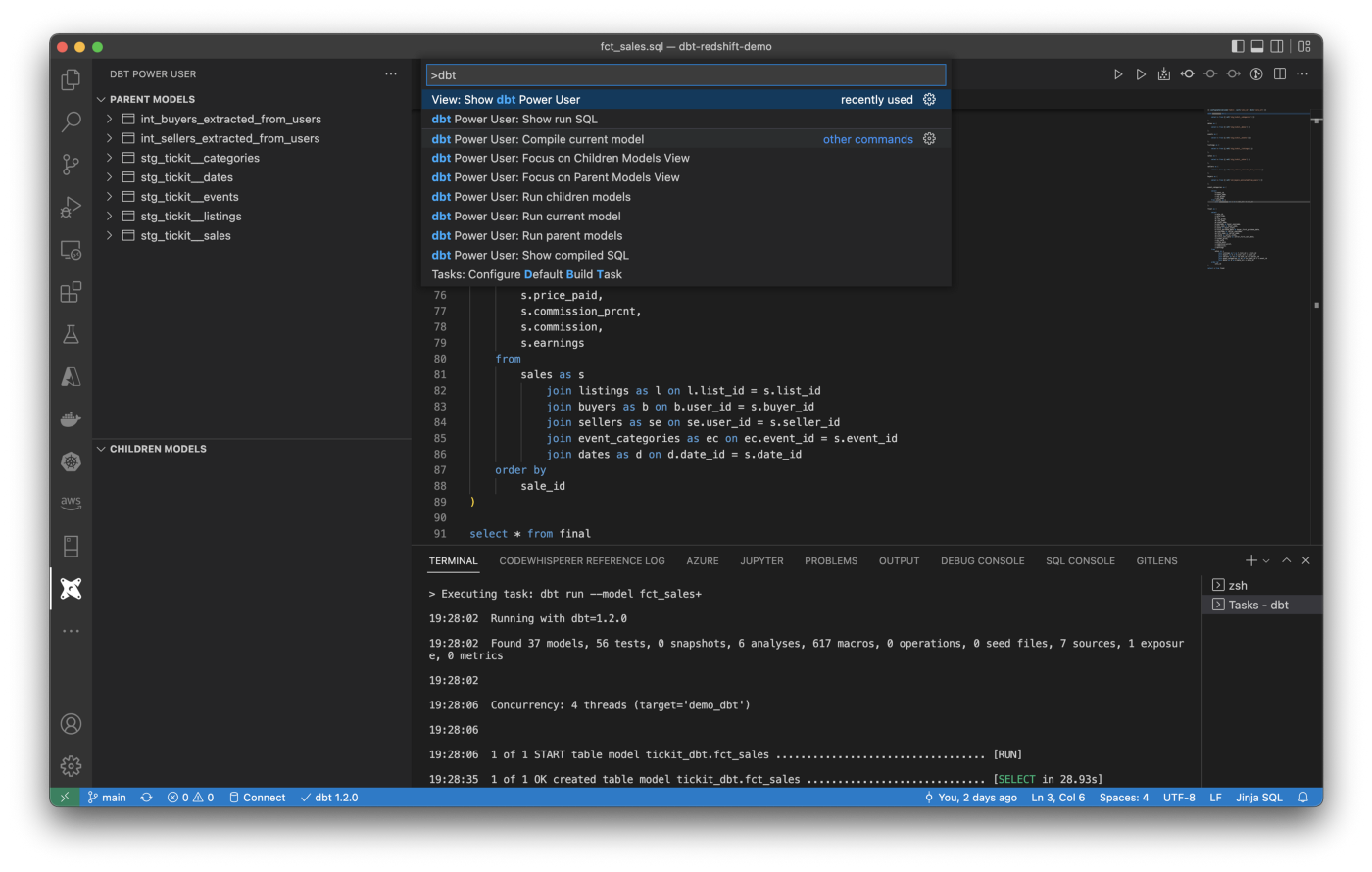
- Microsoft Visual Studio Code (VS Code) with dbt extensions installed;
The post’s demonstration uses dbt Cloud, VS Code, and the dbt CLI interchangeably with the project’s GitHub repository as a source. Follow along with the demonstration using any or all of these three dbt options.
Cost Warning!
Be careful when creating a new, provisioned Amazon Redshift cluster for this demonstration. The suggested default Production cluster with two ra3.4xlarge on-demand compute nodes and AQUA (Redshift’s Advanced Query Accelerator) enabled is estimated at $4,694/month ($3.26/node/hour). For this demonstration, choose the minimum size provisioned Redshift cluster configuration of one dc2.large on-demand compute node, estimated to cost $180/month ($0.25/node/hour). Be sure to delete the cluster when the demonstration is complete.

Amazon Redshift Serverless Option
AWS recently announced the general availability (GA) of Amazon Redshift Serverless on July 12, 2022. Amazon Redshift Serverless allows data analysts, developers, and data scientists to run and scale analytics without having to provision and manage data warehouse clusters. dbt is fully compatible with Amazon Redshift Serverless and is an alternative to provisioned Redshift for this demonstration. According to AWS, Amazon Redshift Serverless measures data warehouse capacity in Redshift Processing Units (RPUs). You pay for the workloads you run in RPU-hours on a per-second basis (with a 60-second minimum charge), including queries that access data in open file formats in Amazon S3.
Source Code
All the source code demonstrated in this post is open source and available on GitHub.
Sample Data
This demonstration uses the TICKIT sample database provided by AWS and designed for use with Amazon Redshift. This sample database application tracks sales activity for the fictional online TICKIT website, where users buy and sell tickets for sporting events, shows, and concerts. The database consists of seven tables in a star schema: five dimension tables and two fact tables. A clean copy of the raw TICKIT data, formatted as pipe-delimited text files, is included in this GitHub project. Use the following shell commands to copy the raw data to Amazon S3:
Prepare Amazon Redshift for dbt
Create New Database
Create a new Redshift database to use for the demonstration, demo.
Create Database Schemas
Within the new Redshift database,demo, create the external schema, tickit_external, and the corresponding external AWS Glue Data Catalog, tickit_dbt, using the CREATE EXTERNAL SCHEMA Redshift SQL command. Make sure to update the command to reflect your IAM Role’s ARN. Next, create the schema that will hold our dbt models, tickit_dbt. Lastly, as a security best practice, drop the default public schema.
From the AWS Glue console, we should observe a new tickit_dbt AWS Glue Data Catalog. The description shown below was manually added after the catalog was created.

Create dbt Database User and Group
As a security best practice, create a separate database dbt user and dbt group. We are assigning a completely arbitrary connection limit of ten. Then, apply the grants to allow the dbt group access to the new database and schemas. Lastly, change the two schema’s owners to the dbt.
Alternately, we could use an IAM Role with a SAML 2.0-compliant IdP.
Initialize and Configure dbt for Redshift
Next, configure your dbt Cloud account and dbt locally with your Amazon Redshift connection information using the dbt init command. On a Mac, this configuration is stored in the /Users/<your_usernama>/.dbt/profiles.yml file. You will need your Redshift cluster host URL, port, database, username, and password. With your local install of dbt, we can use the dbt debug command to confirm the new configuration.

Project Structure
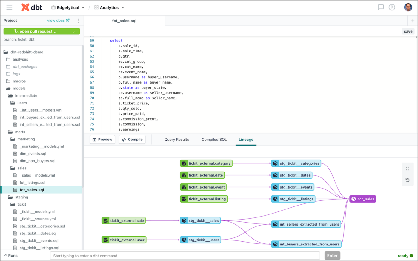
The GitHub project structure follows many of the best practices outlined in dbt Labs’ Best Practice Guide. Data models in the models directory is organized into the recommended staging, intermediate, and marts subdirectories (aka layers).

From a data lineage perspective, in this project, the staging layer’s data models depend on the external tables (AWS Glue/Amazon Redshift Spectrum). The intermediate layer’s data models depend on the staging models. The marts layer’s data models depend on staging and intermediate models.

Install dbt Packages
The GitHub project’s packages.yml contains a few commonly recommended packages. The only one required for this post is the dbt-labs/dbt_external_tables package. Make sure your project is referring to the latest version of the package.
Use the dbt deps command to install the packages locally.

External Tables
The _tickit__sources.yml file in the models/staging/tickit/external_tables/ model’s subdirectory defines the schema and S3 location for each of the seven external TICKIT database tables: category, date, event, listing, sale, user, and venue. You will need to update this file to reflect the name of your Amazon S3 bucket, in seven places.
Execute the command, dbt run-operation stage_external_sources, to create the seven external tables in the AWS Glue Data Catalog. This command is part of the dbt_external_tables package we installed earlier. It iterates through all source nodes, creates the tables if missing, and refreshes metadata.

If we failed to run the previous SQL statements to set schema ownership to the dbt user, the following error will likely occur.

Once the command completes, we should observe seven new tables in the AWS Glue Data Catalog.

Examining one of the AWS Glue data catalog tables, we can observe how the configuration in the _tickit__sources.yml file was used to define the table’s properties and schema. Note the Location field indicates where the underlying data is located in our Amazon S3 bucket.

Staging Layer
In their best practices guide, dbt describes the staging layer in the following manner: “you can think of the staging layer as condensing and refining this material into the individual atoms we’ll later build more intricate and useful structures with.” The staging data models are the base tables and views we will use to build more complex aggregations and analytics queries in Redshift. The schema.yml file, also in the models/staging/tickit/ model’s subdirectory, defines seven late-binding views, modeled by dbt, to be created in Amazon Redshift.
The staging model’s SQL statements also follow many of dbt’s best practices. Below, we see an example of the stg_tickit__sales model (stg_tickit__sales.sql). This model performs a SELECT from the external sale table in the external_table schema. The model performs column renaming and basic calculations.
The the dbt run command, according to dbt, “executes compiled SQL model files against the current target database. dbt connects to the target database and runs the relevant SQL, required to materialize all data models using the specified materialization strategies.” Instead of using the dbt run command to create all the project’s tables and views at once, for now, we are limiting the command to just the models in the ./models/staging/tickit/ directory using the --select optional argument. Execute the dbt run --select staging command to materialize the seven corresponding staging tables in Amazon Redshift.

Once the command completes, we should observe seven new views in Amazon Redshift demo database’s tickit_dbt schema with the stg_ prefix.

Selecting from any of the views should return data.

Late Binding Views
This demonstration uses late binding views for staging and intermediate layer models. According to dbt, “using late-binding views in a production deployment of dbt can vastly improve the availability of data in the warehouse, especially for models that are materialized as late-binding views and are queried by end-users, since they won’t be dropped when upstream models are updated. Additionally, late binding views can be used with external tables via Redshift Spectrum.”
Alternatively, we could define the seven staging models as tables instead of late binding views. Once created as tables, the dependent intermediate and marts views will not require a late-binding reference, as in this project.
Intermediate Layer
In their best practices guide, dbt describes the intermediate layer as “purpose-built transformation steps.” Further, “the best guiding principle is to think about verbs (e.g. pivoted, aggregated_to_user, joined, fanned_out_by_quanity, funnel_created, etc.) in the intermediate layer.”
The project’s intermediate layer consists of two models related to users. The sample TICKIT database lumps all users into a single table. However, for analytics purposes, different user personas might interest marketing teams, such as buyers, sellers, sellers who also buy, and non-buyers (users who have never purchased tickets). The two models in the project’s intermediate layer filter for buyers and for sellers, resulting in two separate views of user personas.
To materialize the intermediate layer’s two data models into views, execute the command, dbt run --select intermediate.

Once the command completes, we should observe a total of nine views in Amazon Redshift demo database’s tickit_dbt schema — seven staging and two intermediate, identified with the int_ prefix.

Marts Layer
In their best practices guide, dbt describes the marts layer as “business defined entities.” Further, “this is the layer where everything comes together and we start to arrange all of our atoms (staging models) and molecules (intermediate models) into full-fledged cells that have identity and purpose. We sometimes like to call this the entity layer or concept layer, to emphasize that all our marts are meant to represent a specific entity or concept at its unique grain.”
The project’s marts layer consists of four data models across marketing and sales. The models are materialized as two dimension tables and two fact tables. Although it is common practice to describe and label these as traditional star schema dimension (dim_) or fact (fct_) tables, in reality, the fact tables in this demonstration are actually flat, de-normalized, wide tables. Wide tables generally have better analytics performance in a modern data warehouse, according to Fivetran and others.
The marts layer’s models take various dependencies through joins on staging and intermediate models. The data model above, fct_sales, has dependencies on multiple staging and intermediate models.

To materialize the marts layer’s four data models into tables, execute the command, dbt run --select marts.

Once the command completes, we should observe four tables and nine views in the Redshift demo database’s tickit_dbt schema. Note how the dbt model for fct_sales (shown above), with its Jinja templating and multiple CTEs have been compiled into the resulting table in Redshift, this is the real magic of dbt!

At this point, all of the project’s models have been compiled and created in the Redshift demo database by dbt.
Analyses
The demonstration’s project also contains example analyses. dbt allows us to version control more analytical-oriented SQL files within our dbt project using the analyses functionality of dbt. These analyses do not fit the fairly opinionated dbt model definition. We can compile the analyses SQL file using the dbt compile command, then copy and paste the resulting SQL statements from the target/compiled/ subdirectory into our data warehouse’s query tool of choice.

Project Documentation
Using the dbt docs generate command will automatically generate the project’s documentation website from the SQL and YAML files. Documentations can be generated and displayed from your dbt Cloud account or hosted locally.

Testing
According to dbt, “Tests are assertions you make about your models and other resources in your dbt project (e.g. sources, seeds, and snapshots). When you run dbt test, dbt will tell you if each test in your project passes or fails.” The project contains over 50 tests, split between the _tickit__sources.yml file and individual tests in the test/ directory. Typical dbt tests check for non-null and unique values, values within an expected numeric range, and values from a known list of strings. Any SELECT statement written in SQL can be tested.
Execute the project’s tests using the dbt test command. We can execute individual tests using the --select optional argument, for example, dbt test --select assert_all_sale_amounts_are_positive. We can also use the --threads optional argument with most dbt commands, including dbt test, increasing parallelism and reducing execution time. The example below uses 10 threads, the arbitrary maximum configured for the Amazon Redshift dbt user.


Jobs
According to dbt, Jobs are a set of dbt commands that you want to run on a schedule. For example, dbt run and dbt test. Jobs can load packages, run tests, materialize models, check source freshness (dbt source freshness), and regenerate documentation. Below, we have created a daily job to test, refresh, and document our project as the data is updated in the data lake.

Notifications
According to dbt, Setting up notifications in dbt Cloud will allow you to receive alerts via Email or a chosen Slack channel when a job run succeeds, fails, or is canceled.

The Slack notifications include run status, timings, and a link to open the job in dbt Cloud. Below, we see a notification regarding our project’s daily job run.

Exposures
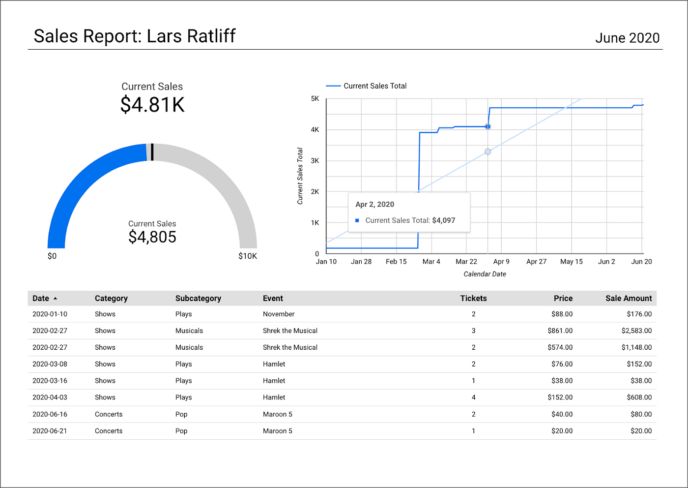
Exposures are a recent addition to dbt. Exposures make it possible to define and describe a downstream use of our dbt project, such as in a dashboard, application, or data science pipeline. Below we see an example of an exposure describing a sales dashboard created in Amazon QuickSight.
The exposure YAML file shown above describes the Amazon QuickSight dashboard shown below.

Exposures work with dbt’s auto-documentation feature. dbt populates a dedicated page in the auto-generated documentation site with context relevant to data consumers.


Conclusion
In this post, we covered some of the basic functionality of dbt. We learned how dbt enables analysts to work more like software engineers. We also learned how dbt makes it easy to codify data models in SQL, to version control and manage data models as code with git, and collaborate on data models with other data team members.
Topics not explored in this post but critical to most large-scale dbt-managed production environments include advanced Jinja templating and macros, model freshness, orchestration, job scheduling, Continuous Integration and GitOps, notifications, environment variables, and incremental models. We will explore these additional dbt capabilities in future posts.
This blog represents my viewpoints and not of my employer, Amazon Web Services (AWS). All product names, logos, and brands are the property of their respective owners. All diagrams and illustrations are the property of the author unless otherwise noted.
Serverless Analytics on AWS: Getting Started with Amazon EMR Serverless and Amazon MSK Serverless
Utilizing the recently released Amazon EMR Serverless and Amazon MSK Serverless for batch and streaming analytics with Apache Spark and Apache Kafka
Introduction
Amazon EMR Serverless
AWS recently announced the general availability (GA) of Amazon EMR Serverless on June 1, 2022. EMR Serverless is a new serverless deployment option in Amazon EMR, in addition to EMR on EC2, EMR on EKS, and EMR on AWS Outposts. EMR Serverless provides a serverless runtime environment that simplifies the operation of analytics applications that use the latest open source frameworks, such as Apache Spark and Apache Hive. According to AWS, with EMR Serverless, you don’t have to configure, optimize, secure, or operate clusters to run applications with these frameworks.
Amazon MSK Serverless
Similarly, on April 28, 2022, AWS announced the general availability of Amazon MSK Serverless. According to AWS, Amazon MSK Serverless is a cluster type for Amazon MSK that makes it easy to run Apache Kafka without managing and scaling cluster capacity. MSK Serverless automatically provisions and scales compute and storage resources, so you can use Apache Kafka on demand and only pay for the data you stream and retain.
Serverless Analytics
In the following post, we will learn how to use these two new, powerful, cost-effective, and easy-to-operate serverless technologies to perform batch and streaming analytics. The PySpark examples used in this post are similar to those featured in two earlier posts, which featured non-serverless alternatives Amazon EMR on EC2 and Amazon MSK: Getting Started with Spark Structured Streaming and Kafka on AWS using Amazon MSK and Amazon EMR and Stream Processing with Apache Spark, Kafka, Avro, and Apicurio Registry on AWS using Amazon MSK and EMR.
Source Code
All the source code demonstrated in this post is open-source and available on GitHub.
git clone --depth 1 -b main \
    https://github.com/garystafford/emr-msk-serverless-demo.git
Architecture
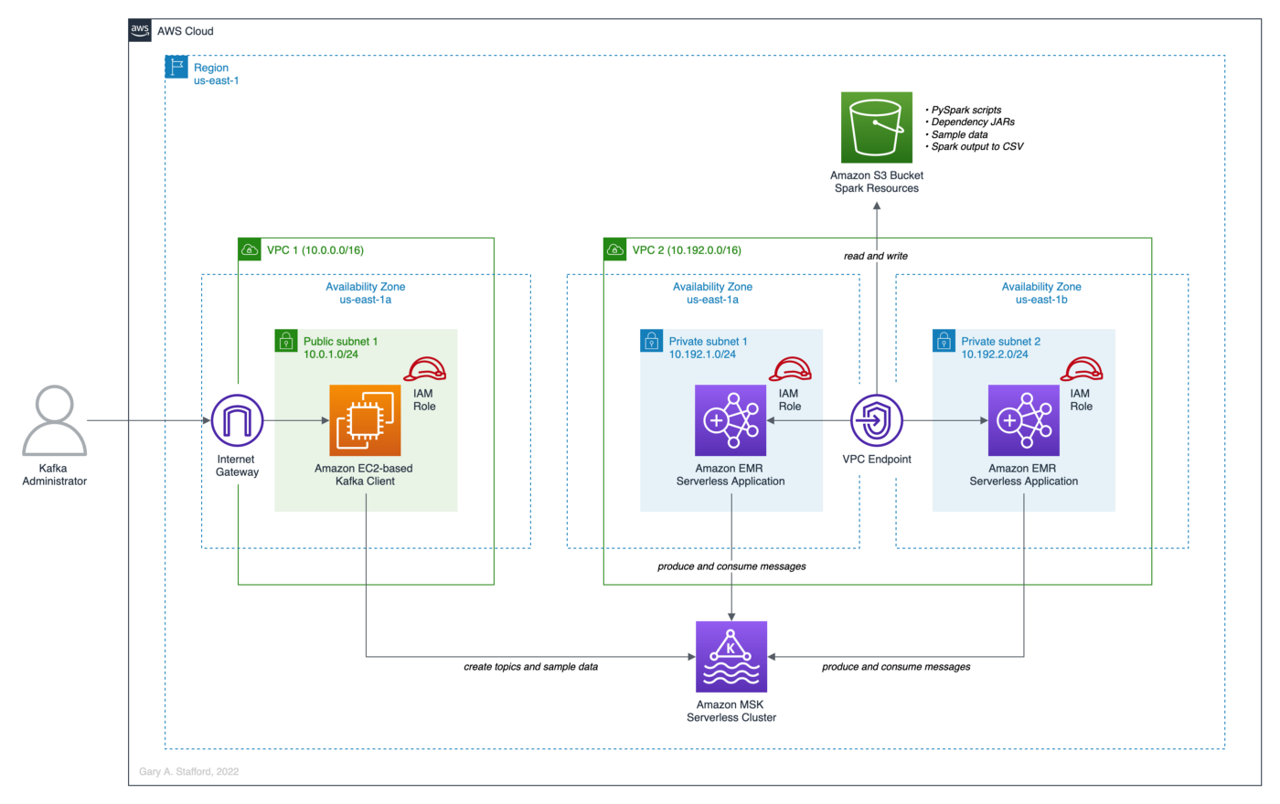
The post’s high-level architecture consists of an Amazon EMR Serverless Application, Amazon MSK Serverless Cluster, and Amazon EC2 Kafka client instance. To support these three resources, we will need two Amazon Virtual Private Clouds (VPCs), a minimum of three subnets, an AWS Internet Gateway (IGW) or equivalent, an Amazon S3 Bucket, multiple AWS Identity and Access Management (IAM) Roles and Policies, Security Groups, and Route Tables, and a VPC Gateway Endpoint for S3. All resources are constrained to a single AWS account and a single AWS Region, us-east-1.
Prerequisites
As a prerequisite for this post, you will need to create the following resources:
- (1) Amazon EMR Serverless Application;
- (1) Amazon MSK Serverless Cluster;
- (1) Amazon S3 Bucket;
- (1) VPC Endpoint for S3;
- (3) Apache Kafka topics;
- PySpark applications, related JAR dependencies, and sample data files uploaded to Amazon S3 Bucket;
Let’s walk through each of these prerequisites.
Amazon EMR Serverless Application
Before continuing, I suggest familiarizing yourself with the AWS documentation for Amazon EMR Serverless, especially, What is Amazon EMR Serverless? Create a new EMR Serverless Application by following the AWS documentation, Getting started with Amazon EMR Serverless. The creation of the EMR Serverless Application includes the following resources:
- Amazon S3 bucket for storage of Spark resources;
- Amazon VPC with at least two private subnets and associated Security Group(s);
- EMR Serverless runtime AWS IAM Role and associated IAM Policy;
- Amazon EMR Serverless Application;
For this post, use the latest version of EMR available in the EMR Studio Serverless Application console, the newly released version 6.7.0, to create a Spark application.

Keep the default pre-initialized capacity, application limits, and application behavior settings.

Since we are connecting to MSK Serverless from EMR Serverless, we need to configure VPC access. Select the new VPC and at least two private subnets in different Availability Zones (AZs).

According to the documentation, the subnets selected for EMR Serverless must be private subnets. The associated route tables for the subnets should not contain direct routes to the Internet.


Amazon MSK Serverless Cluster
Similarly, before continuing, I suggest familiarizing yourself with the AWS documentation for Amazon MSK Serverless, especially MSK Serverless. Create a new MSK Serverless Cluster by following the AWS documentation, Getting started using MSK Serverless clusters. The creation of the MSK Serverless Cluster includes the following resources:
- AWS IAM Role and associated IAM Policy for the Amazon EC2 Kafka client instance;
- VPC with at least one public subnet and associated Security Group(s);
- Amazon EC2 instance used as Apache Kafka client, provisioned in the public subnet of the above VPC;
- Amazon MSK Serverless Cluster;

Associate the new MSK Serverless Cluster with the EMR Serverless Application’s VPC and two private subnets. Also, associate the cluster with the EC2-based Kafka client instance’s VPC and its public subnet.


According to the AWS documentation, Amazon MSK does not support all AZs. For example, I tried to use a subnet in us-east-1e threw an error. If this happens, choose an alternative AZ.


VPC Endpoint for S3
To access the Spark resource in Amazon S3 from EMR Serverless running in the two private subnets, we need a VPC Endpoint for S3. Specifically, a Gateway Endpoint, which sends traffic to Amazon S3 or DynamoDB using private IP addresses. A gateway endpoint for Amazon S3 enables you to use private IP addresses to access Amazon S3 without exposure to the public Internet. EMR Serverless does not require public IP addresses, and you don’t need an internet gateway (IGW), a NAT device, or a virtual private gateway in your VPC to connect to S3.

Create the VPC Endpoint for S3 (Gateway Endpoint) and add the route table for the two EMR Serverless private subnets. You can add additional routes to that route table, such as VPC peering connections to data sources such as Amazon Redshift or Amazon RDS. However, do not add routes that provide direct Internet access.

Kafka Topics and Sample Messages
Once the MSK Serverless Cluster and EC2-based Kafka client instance are provisioned and running, create the three required Kafka topics using the EC2-based Kafka client instance. I recommend using AWS Systems Manager Session Manager to connect to the client instance as the ec2-user user. Session Manager provides secure and auditable node management without the need to open inbound ports, maintain bastion hosts, or manage SSH keys. Alternatively, you can SSH into the client instance.

Before creating the topics, use a utility like telnet to confirm connectivity between the Kafka client and the MSK Serverless Cluster. Verifying connectivity will save you a lot of frustration with potential security and networking issues.
With MSK Serverless Cluster connectivity confirmed, create the three Kafka topics: topicA, topicB, and topicC. I am using the default partitioning and replication settings from the AWS Getting Started Tutorial.
To create some quick sample data, we will copy and paste 250 messages from a file included in the GitHub project, sample_data/sales_messages.txt, into topicA. The messages are simple mock sales transactions.
Use the kafka-console-producer Shell script to publish the messages to the Kafka topic. Use the kafka-console-consumer Shell script to validate the messages made it to the topic by consuming a few messages.
The output should look similar to the following example.

Spark Resources in Amazon S3
To submit and run the five Spark Jobs included in the project, you will need to copy the following resources to your Amazon S3 bucket: (5) Apache Spark jobs, (5) related JAR dependencies, and (2) sample data files.
PySpark Applications
To start, copy the five PySpark applications to a scripts/ subdirectory within your Amazon S3 bucket.

Sample Data
Next, copy the two sample data files to a sample_data/ subdirectory within your Amazon S3 bucket. The large file contains 2,000 messages, while the small file contains 600 messages. These two files can be used interchangeably with the post’s final streaming example.

PySpark Dependencies
Lastly, the PySpark applications have a handful of JAR dependencies that must be available when the job runs, which are not on the EMR Serverless classpath by default. If you are unsure which JARs are already on the EMR Serverless classpath, you can check the Spark UI’s Environment tab’s Classpath Entries section. Accessing the Spark UI is demonstrated in the first PySpark application example, below.

It is critical to choose the correct version of each JAR dependency based on the version of libraries used with the EMR and MSK. Using the wrong version or inconsistent versions, especially Scala, can result in job failures. Specifically, we are targeting Spark 3.2.1 and Scala 2.12 (EMR v6.7.0: Amazon’s Spark 3.2.1, Scala 2.12.15, Amazon Corretto 8 version of OpenJDK), and Apache Kafka 2.8.1 (MSK Serverless: Kafka 2.8.1).
Download the seven JAR files locally, then copy them to a jars/ subdirectory within your Amazon S3 bucket.

PySpark Applications Examples
With the EMR Serverless Application, MSK Serverless Cluster, Kafka topics, and sample data created, and the Spark resources uploaded to Amazon S3, we are ready to explore four different Spark examples.
Example 1: Kafka Batch Aggregation to the Console
The first PySpark application, 01_example_console.py, reads the same 250 sample sales messages from topicA you published earlier, aggregates the messages, and writes the total sales and quantity of orders by country to the console (stdout).
There are no hard-coded values in any of the PySpark application examples. All required environment-specific variables, such as your MSK Serverless bootstrap server (host and port) and Amazon S3 bucket name, will be passed to the running Spark jobs as arguments from the spark-submit command.
To submit your first PySpark job to the EMR Serverless Application, use the emr-serverless API from the AWS CLI. You will need (4) values: 1) your EMR Serverless Application’s application-id, 2) the ARN of your EMR Serverless Application’s execution IAM Role, 3) your MSK Serverless bootstrap server (host and port), and 4) the name of your Amazon S3 bucket containing the Spark resources.
Switching to the EMR Serverless Application console, you should see the new Spark job you just submitted in one of several job states.

You can click on the Spark job to get more details. Note the Script arguments and Spark properties passed in from the spark-submit command.

From the Spark job details tab, access the Spark UI, aka Spark Web UI, from a button in the upper right corner of the screen. If you have experience with Spark, you are most likely familiar with the Spark Web UI to monitor and tune Spark jobs.

From the initial screen, the Spark History Server tab, click on the App ID. You can access an enormous amount of Spark-related information about your job and EMR environment from the Spark Web UI.


The Executors tab will give you access to the Spark job’s output. The output we are most interested in is the driver executor’s stderr and stdout (first row of the second table, shown below).

The stderr contains output related to the running Spark job. Below we see an example of Kafka consumer configuration values output to stderr. Several of these values were passed in from the Spark job, including items such as kafka.bootstrap.servers, security.protocol, sasl.mechanism, and sasl.jaas.config.

The stdout from the driver executor contains the console output as directed from the Spark job. Below we see the successfully aggregated results of the first Spark job, output to stdout.
Example 2: Kafka Batch Aggregation to CSV in S3
Although the console is useful for development and debugging, it is typically not used in Production. Instead, Spark typically sends results to S3 as CSV, JSON, Parquet, or Arvo formatted files, to Kafka, to a database, or to an API endpoint. The second PySpark application, 02_example_csv_s3.py, reads the same 250 sample sales messages from topicA you published earlier, aggregates the messages, and writes the total sales and quantity of orders by country to a CSV file in Amazon S3.
To submit your second PySpark job to the EMR Serverless Application, use the emr-serverless API from the AWS CLI. Similar to the first example, you will need (4) values: 1) your EMR Serverless Application’s application-id, 2) the ARN of your EMR Serverless Application’s execution IAM Role, 3) your MSK Serverless bootstrap server (host and port), and 4) the name of your Amazon S3 bucket containing the Spark resources.
If successful, the Spark job should create a single CSV file in the designated Amazon S3 key (directory path) and an empty _SUCCESS indicator file. The presence of an empty _SUCCESS file signifies that the save() operation completed normally.

Below we see the expected pipe-delimited output from the second Spark job.
Example 3: Kafka Batch Aggregation to Kafka
The third PySpark application, 03_example_kafka.py, reads the same 250 sample sales messages from topicA you published earlier, aggregates the messages, and writes the total sales and quantity of orders by country to a second Kafka topic, topicB. This job now has both read and write options.
To submit your next PySpark job to the EMR Serverless Application, use the emr-serverless API from the AWS CLI. Similar to the first two examples, you will need (4) values: 1) your EMR Serverless Application’s application-id, 2) the ARN of your EMR Serverless Application’s execution IAM Role, 3) your MSK Serverless bootstrap server (host and port), and 4) the name of your Amazon S3 bucket containing the Spark resources.
Once the job completes, you can confirm the results by returning to your EC2-based Kafka client. Use the same kafka-console-consumer command you used previously to show messages from topicB.
If the Spark job and the Kafka client command worked successfully, you should see aggregated messages similar to the example output below. Note we are not using keys with the Kafka messages, only values for these simple examples.

Example 4: Spark Structured Streaming
For our final example, we will switch from batch to streaming — from read to readstream and from write to writestream. Before continuing, I suggest reading the Structured Streaming Programming Guide.
In this example, we will demonstrate how to continuously measure a common business metric — real-time sales volumes. Imagine you are sell products globally and want to understand the relationship between the time of day and buying patterns in different geographic regions in real-time. For any given window of time — this 15-minute period, this hour, this day, or this week— you want to know the current sales volumes by country. You are not reviewing previous sales periods or examing running sales totals, but real-time sales during a sliding time window.
We will use two PySpark jobs running concurrently to simulate this metric. The first application, 04_stream_sales_to_kafka.py, simulates streaming data by continuously writing messages to topicC — 2,000 messages with a 0.5-second delay between messages. In my tests, the job ran for ~28–29 minutes.
Simultaneously, the PySpark application, 05_streaming_kafka.py, continuously consumes the sales transaction messages from the same topic, topicC. Then, Spark aggregates messages over a sliding event-time window and writes the results to the console.
To submit the two PySpark jobs to the EMR Serverless Application, use the emr-serverless API from the AWS CLI. Again, you will need (4) values: 1) your EMR Serverless Application’s application-id, 2) the ARN of your EMR Serverless Application’s execution IAM Role, 3) your MSK Serverless bootstrap server (host and port), and 4) the name of your Amazon S3 bucket containing the Spark resources.
Switching to the EMR Serverless Application console, you should see both Spark jobs you just submitted in one of several job states.

Using the Spark UI again, we can review the output from the second job, 05_streaming_kafka.py.

With Spark Structured Streaming jobs, we have an extra tab in the Spark UI, Structured Streaming. This tab displays all running jobs with their latest [micro]batch number, the aggregate rate of data arriving, and the aggregate rate at which Spark is processing data. Unfortunately, with MSK Serverless, AWS doesn’t appear to allow access to the detailed streaming query statistics via the Run ID, which greatly reduces its value. You receive a 502 error when clicking on the Run ID hyperlink.

The output we are most interested in, again, is contained in the driver executor’s stderr and stdout (first row of the second table, shown below).

Below we see sample output from stderr. The output shows the results of a micro-batch. According to the Apache Spark documentation, internally, by default, Structured Streaming queries are processed using a micro-batch processing engine. The engine processes data streams as a series of small batch jobs, achieving end-to-end latencies as low as 100ms and exactly-once fault-tolerance guarantees.
The corresponding output to the micro-batch output above is shown below. We see the initial micro-batch results, starting with the first micro-batch before any messages are streamed to topicC.
If you are familiar with Spark Structured Streaming, you are likely aware that these Spark jobs run continuously. In other words, the streaming jobs will not stop; they continually await more streaming data.

The first job, 04_stream_sales_to_kafka.py, will run for ~28–29 minutes and stop with a status of Sucess. However, the second job, 05_streaming_kafka.py, the Spark Structured Streaming job, must be manually canceled.

Cleaning Up
You can delete your resources from the AWS Management Console or AWS CLI. However, to delete your Amazon S3 bucket, all objects (including all object versions and delete markers) in the bucket must be deleted before the bucket itself can be deleted.
Conclusion
In this post, we discovered how easy it is to adopt a serverless approach to Analytics on AWS. With EMR Serverless, you don’t have to configure, optimize, secure, or operate clusters to run applications with these frameworks. With MSK Serverless, you can use Apache Kafka on demand and pay for the data you stream and retain. In addition, MSK Serverless automatically provisions and scales compute and storage resources. Given suitable analytics use cases, EMR Serverless with MSK Serverless will likely save you time, effort, and expense.
This blog represents my viewpoints and not of my employer, Amazon Web Services (AWS). All product names, logos, and brands are the property of their respective owners. All diagrams and illustrations are the property of the author unless otherwise noted.
Utilizing In-memory Data Caching to Enhance the Performance of Data Lake-based Applications
Posted by Gary A. Stafford in Analytics, AWS, Big Data, Cloud, Java Development, Software Development, SQL on July 12, 2022
Significantly improve the performance and reduce the cost of data lake-based analytics applications using Amazon ElastiCache for Redis
Introduction
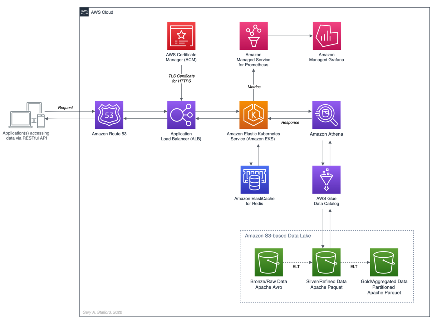
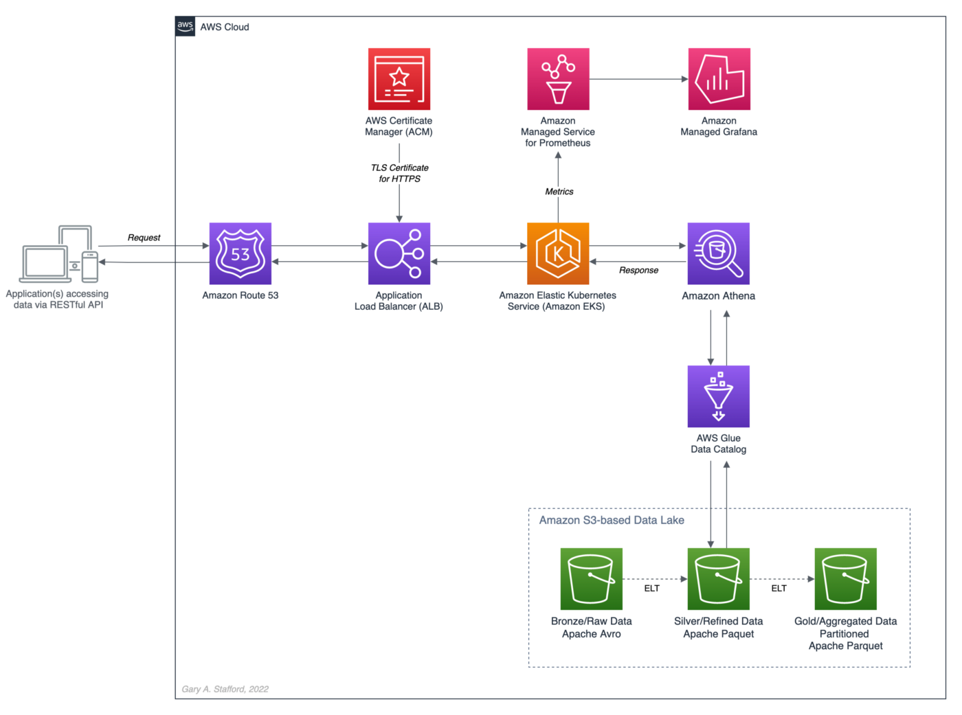
The recent post, Developing Spring Boot Applications for Querying Data Lakes on AWS using Amazon Athena, demonstrated how to develop a Cloud-native analytics application using Spring Boot. The application queried data in an Amazon S3-based data lake via an AWS Glue Data Catalog utilizing the Amazon Athena API.
Securely exposing data in a data lake using RESTful APIs can fulfill many data-consumer needs. However, access to that data can be significantly slower than access from a database or data warehouse. For example, in the previous post, we imported the OpenAPI v3 specification from the Spring Boot service into Postman. The API specification contained approximately 17 endpoints.
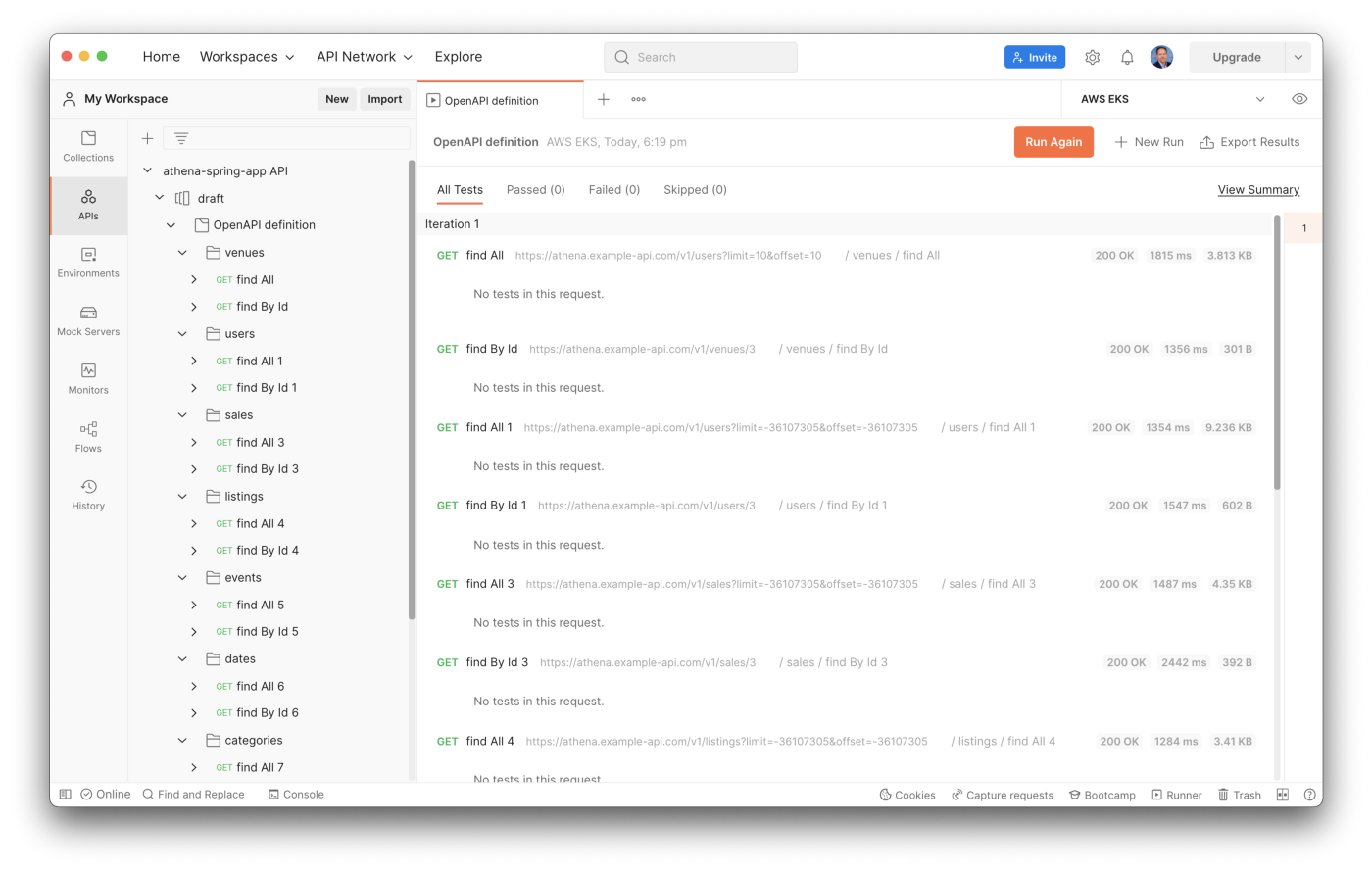
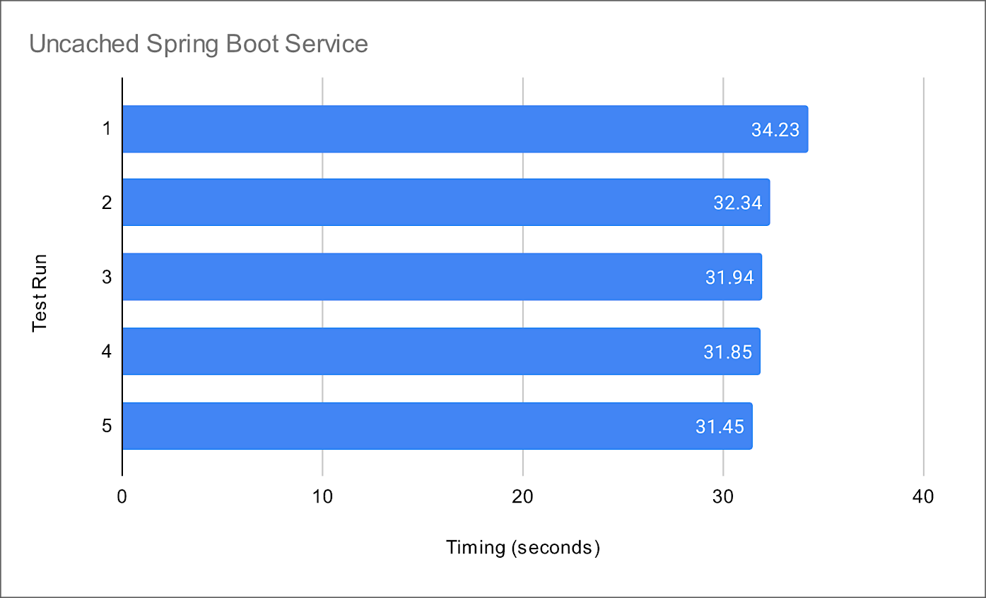
From my local development laptop, the Postman API test run times for all service endpoints took an average of 32.4 seconds. The Spring Boot service was running three Kubernetes pod replicas on Amazon EKS in the AWS US East (N. Virginia) Region.
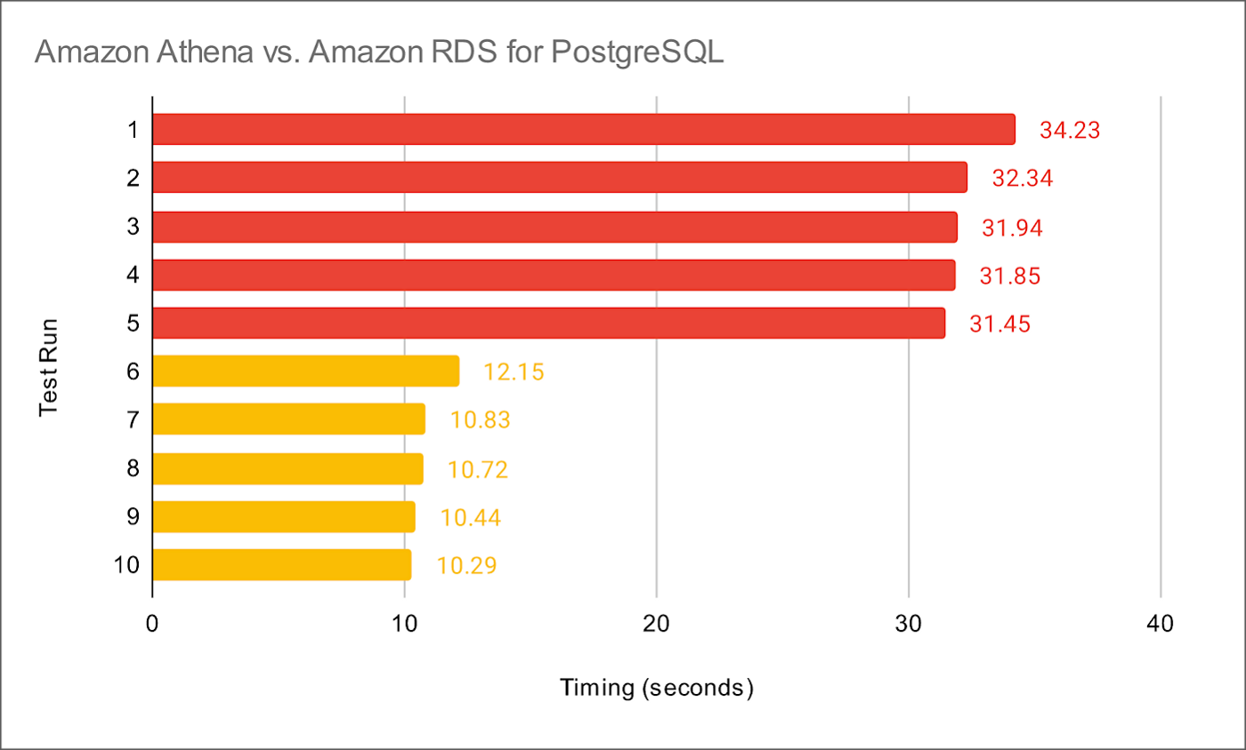
Compare the data lake query result times to equivalent queries made against a minimally-sized Amazon RDS for PostgreSQL database instance containing the same data. The average run times for all PostgreSQL queries averaged 10.8 seconds from a similar Spring Boot service. Although not a precise benchmark, we can clearly see that access to the data in the Amazon S3-based data lake is substantially slower, approximately 3x slower, than that of the PostgreSQL database. Tuning the database would easily create an even greater disparity.
Caching for Data Lakes
According to AWS, the speed and throughput of a database can be the most impactful factor for overall application performance. Consequently, in-memory data caching can be one of the most effective strategies to improve overall application performance and reduce database costs. This same caching strategy can be applied to analytics applications built atop data lakes, as this post will demonstrate.
In-memory Caching
According to Hazelcast, memory caching (aka in-memory caching), often simply referred to as caching, is a technique in which computer applications temporarily store data in a computer’s main memory (e.g., RAM) to enable fast retrievals of that data. The RAM used for the temporary storage is known as the cache. As an application tries to read data, typically from a data storage system like a database, it checks to see if the desired record already exists in the cache. If it does, the application will read the data from the cache, thus eliminating the slower access to the database. If the desired record is not in the cache, then the application reads the record from the source. When it retrieves that data, it writes it to the cache so that when the application needs that same data in the future, it can quickly retrieve it from the cache.
Further, according to Hazelcast, as an application tries to read data, typically from a data storage system like a database, it checks to see if the desired record already exists in the cache. If it does, the application will read the data from the cache, thus eliminating the slower access to the database. If the desired record is not in the cache, then the application reads the record from the source. When it retrieves that data, it writes it to the cache so that when the application needs that same data in the future, it can quickly retrieve it from the cache.
Redis In-memory Data Store
According to their website, Redis is the open-source, in-memory data store used by millions of developers as a database, cache, streaming engine, and message broker. Redis provides data structures such as strings, hashes, lists, sets, sorted sets with range queries, bitmaps, hyperloglogs, geospatial indexes, and streams. In addition, Redis has built-in replication, Lua scripting, LRU eviction, transactions, and different levels of on-disk persistence and provides high availability via Redis Sentinel and automatic partitioning with Redis Cluster.
Amazon ElastiCache for Redis
According to AWS, Amazon ElastiCache for Redis, the fully-managed version of Redis, according to AWS, is a blazing fast in-memory data store that provides sub-millisecond latency to power internet-scale real-time applications. Redis applications can work seamlessly with ElastiCache for Redis without any code changes. ElastiCache for Redis combines the speed, simplicity, and versatility of open-source Redis with manageability, security, and scalability from AWS. As a result, Redis is an excellent choice for implementing a highly available in-memory cache to decrease data access latency, increase throughput, and ease the load on relational and NoSQL databases.
ElastiCache Performance Results
In the following post, we will add in-memory caching to the Spring Boot service introduced in the previous post. In preliminary tests with Amazon ElastiCache for Redis, the Spring Boot service delivered a 34x improvement in average response times. For example, test runs with the best-case scenario of a Redis cache hit ratio of 100% averaged 0.95 seconds compared to 32.4 seconds without Redis.

Source Code
All the source code and Docker and Kubernetes resources are open-source and available on GitHub.
git clone --depth 1 -b redis \
    https://github.com/garystafford/athena-spring-app.git
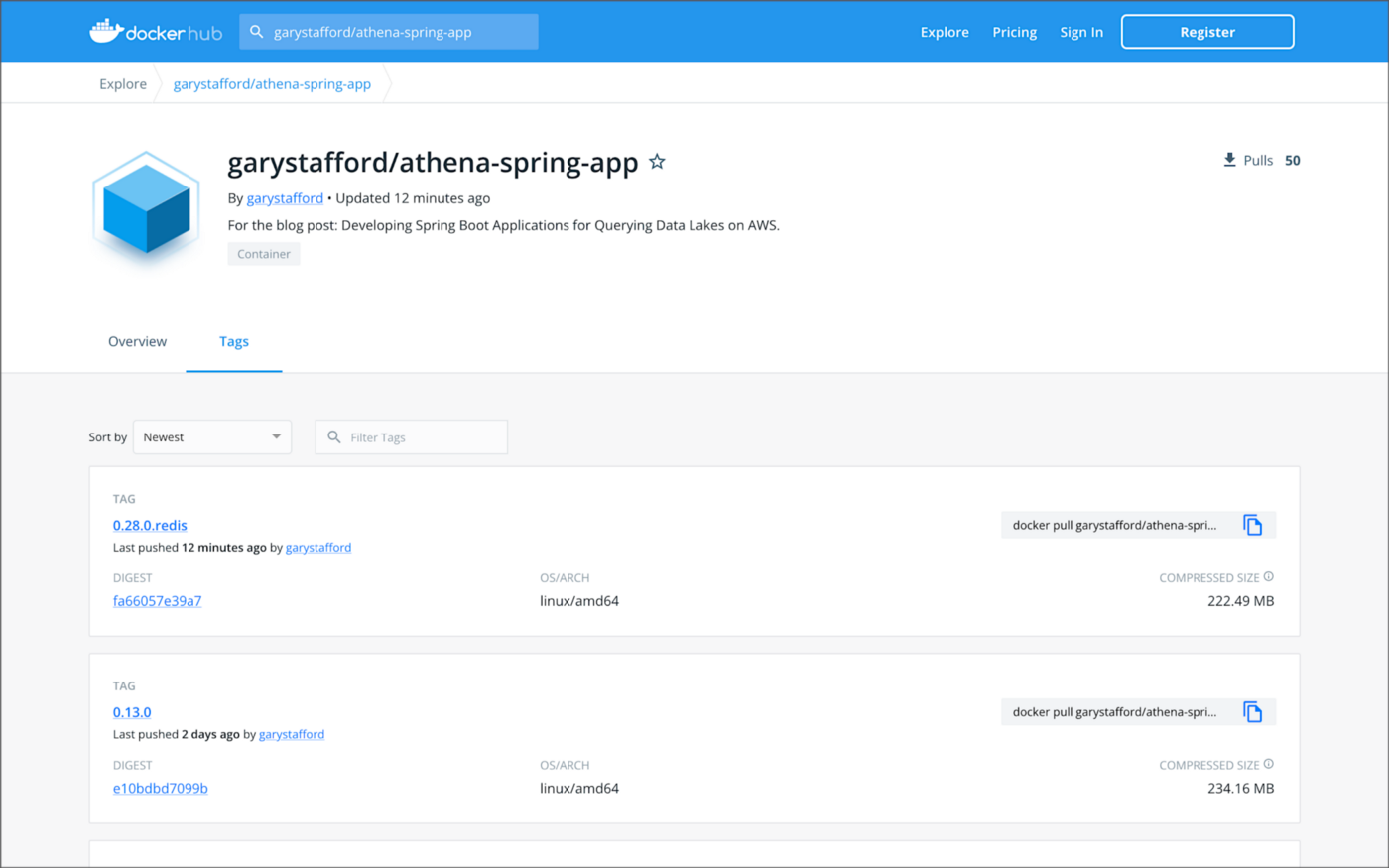
In addition, a Docker image for the Redis-base Spring Boot service is available on Docker Hub. For this post, use the latest tag with the .redis suffix.
Code Changes
The following code changes are required to the Spring Boot service to implement Spring Boot Cache with Redis.
Gradle Build
The gradle.build file now implements two additional dependencies, Spring Boot’s spring-boot-starter-cache and spring-boot-starter-data-redis (lines 45–46).
Application Properties
The application properties file, application.yml, has been modified for both the dev and prod Spring Profiles. The dev Spring Profile expects Redis to be running on localhost. Correspondingly, the project’s docker-compose.yml file now includes a Redis container for local development. The time-to-live (TTL) for all Redis caches is arbitrarily set to one minute for dev and five minutes for prod. To increase application performance and reduce the cost of querying the data lake using Athena, increase Redis’s TTL. Note that increasing the TTL will reduce data freshness.
Athena Application Class
The AthenaApplication class declaration is now decorated with Spring Framework’s EnableCaching annotation (line 22). Additionally, two new Beans have been added (lines 58–68). Spring Redis provides an implementation for the Spring cache abstraction through the org.springframework.data.redis.cache package. The RedisCacheManager cache manager creates caches by default upon the first write. The RedisCacheConfiguration cache configuration helps to customize RedisCache behavior such as caching null values, cache key prefixes, and binary serialization.
POJO Data Model Classes
Spring Boot Redis caching uses Java serialization and deserialization. Therefore, all the POJO data model classes must implement Serializable (line 14).
Service Classes
Each public method in the Service classes is now decorated with Spring Framework’s Cachable annotation (lines 42 and 66). For example, the findById(int id) method in the CategoryServiceImp class is annotated with @Cacheable(value = "categories", key = "#id"). The method’s key parameter uses Spring Expression Language (SpEL) expression for computing the key dynamically. Default is null, meaning all method parameters are considered as a key unless a custom keyGenerator has been configured. If no value is found in the Redis cache for the computed key, the target method will be invoked, and the returned value will be stored in the associated cache.
Controller Classes
There are no changes required to the Controller classes.
Amazon ElastiCache for Redis
Multiple options are available for creating an Amazon ElastiCache for Redis cluster, including cluster mode, multi-AZ option, auto-failover option, node type, number of replicas, number of shards, replicas per shard, Availability Zone placements, and encryption at rest and encryption in transit options. The results in this post are based on a minimally-configured Redis version 6.2.6 cluster, with one shard, two cache.r6g.large nodes, and cluster mode, multi-AZ option, and auto-failover all disabled. In addition, encryption at rest and encryption in transit were also disabled. This cluster configuration is sufficient for development and testing, but not Production.


Testing the Cache
To test Amazon ElastiCache for Redis, we will use Postman again with the imported OpenAPI v3 specification. With all data evicted from existing Redis caches, the first time the Postman tests run, they cause the service’s target methods to be invoked and the returned data stored in the associated caches.
To confirm this caching behavior, use the Redis CLI’s --scan option. To access the redis-cli, I deployed a single Redis pod to Amazon EKS. The first time the --scan command runs, we should get back an empty list of keys. After the first Postman test run, the same --scan command should return a list of cached keys.

Use the Redis CLI’s MONITOR option to further confirm data is being cached, as indicated by the set command.

After the initial caching of data, use the Redis CLI’s MONITOR option, again, to confirm the cache is being hit instead of calling the target methods, which would then invoke the Athena API. Rerunning the Postman tests, we should see get commands as opposed to set commands.

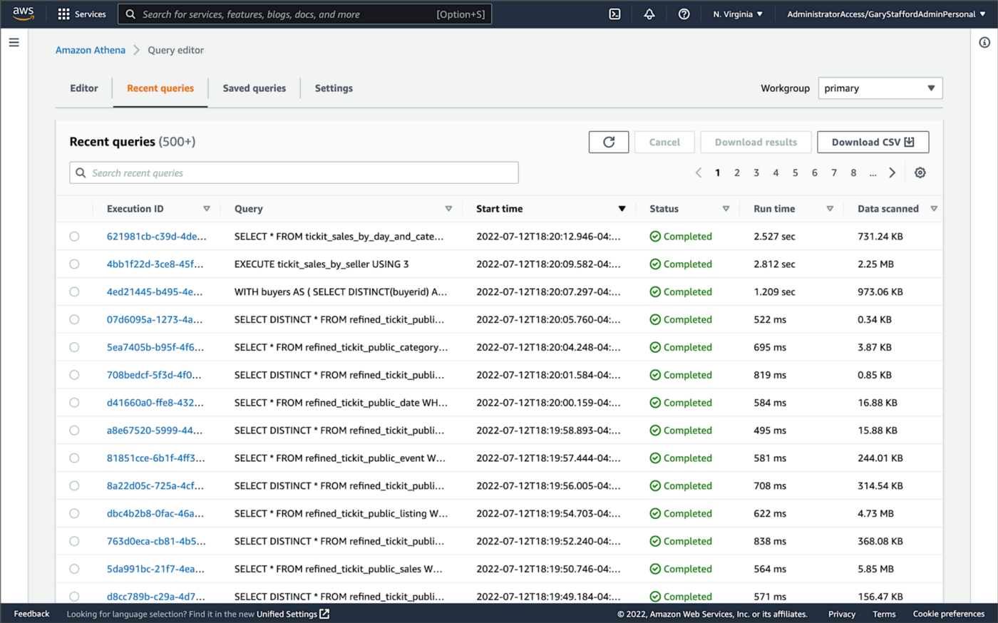
Lastly, to confirm the Spring Boot service is effectively using Redis to cache data, we can also check Amazon Athena’s Recent queries tab in the AWS Management Console. After repeated sequential test runs within the TTL window, we should only see one Athena query per endpoint.
Conclusion
In this brief follow-up to the recent post, Developing Spring Boot Applications for Querying Data Lakes on AWS using Amazon Athena, we saw how to substantially increase data lake application performance using Amazon ElastiCache for Redis. Although this caching technique is often associated with databases, it can also be effectively applied to data lake-based applications, as demonstrated in the post.
This blog represents my viewpoints and not of my employer, Amazon Web Services (AWS). All product names, logos, and brands are the property of their respective owners. All diagrams and illustrations are property of the author unless otherwise noted.
Developing Spring Boot Applications for Querying Data Lakes on AWS using Amazon Athena
Posted by Gary A. Stafford in Analytics, AWS, Big Data, Cloud, Java Development, Software Development on June 26, 2022
Learn how to develop Cloud-native, RESTful Java services that query data in an AWS-based data lake using Amazon Athena’s API
Introduction
AWS provides a collection of fully-managed services that makes building and managing secure data lakes faster and easier, including AWS Lake Formation, AWS Glue, and Amazon S3. Additional analytics services such as Amazon EMR, AWS Glue Studio, and Amazon Redshift allow Data Scientists and Analysts to run high-performance queries on large volumes of semi-structured and structured data quickly and economically.
What is not always as obvious is how teams develop internal and external customer-facing analytics applications built on top of data lakes. For example, imagine sellers on an eCommerce platform, the scenario used in this post, want to make better marketing decisions regarding their products by analyzing sales trends and buyer preferences. Further, suppose the data required for the analysis must be aggregated from multiple systems and data sources; the ideal use case for a data lake.
salesbyseller endpointIn this post, we will explore an example Java Spring Boot RESTful Web Service that allows end-users to query data stored in a data lake on AWS. The RESTful Web Service will access data stored as Apache Parquet in Amazon S3 through an AWS Glue Data Catalog using Amazon Athena. The service will use Spring Boot and the AWS SDK for Java to expose a secure, RESTful Application Programming Interface (API).
Amazon Athena is a serverless, interactive query service based on Presto, used to query data and analyze big data in Amazon S3 using standard SQL. Using Athena functionality exposed by the AWS SDK for Java and Athena API, the Spring Boot service will demonstrate how to access tables, views, prepared statements, and saved queries (aka named queries).

TL;DR
Do you want to explore the source code for this post’s Spring Boot service or deploy it to Kubernetes before reading the full article? All the source code, Docker, and Kubernetes resources are open-source and available on GitHub.
git clone --depth 1 -b main \
    https://github.com/garystafford/athena-spring-app.git
A Docker image for the Spring Boot service is also available on Docker Hub.

Data Lake Data Source
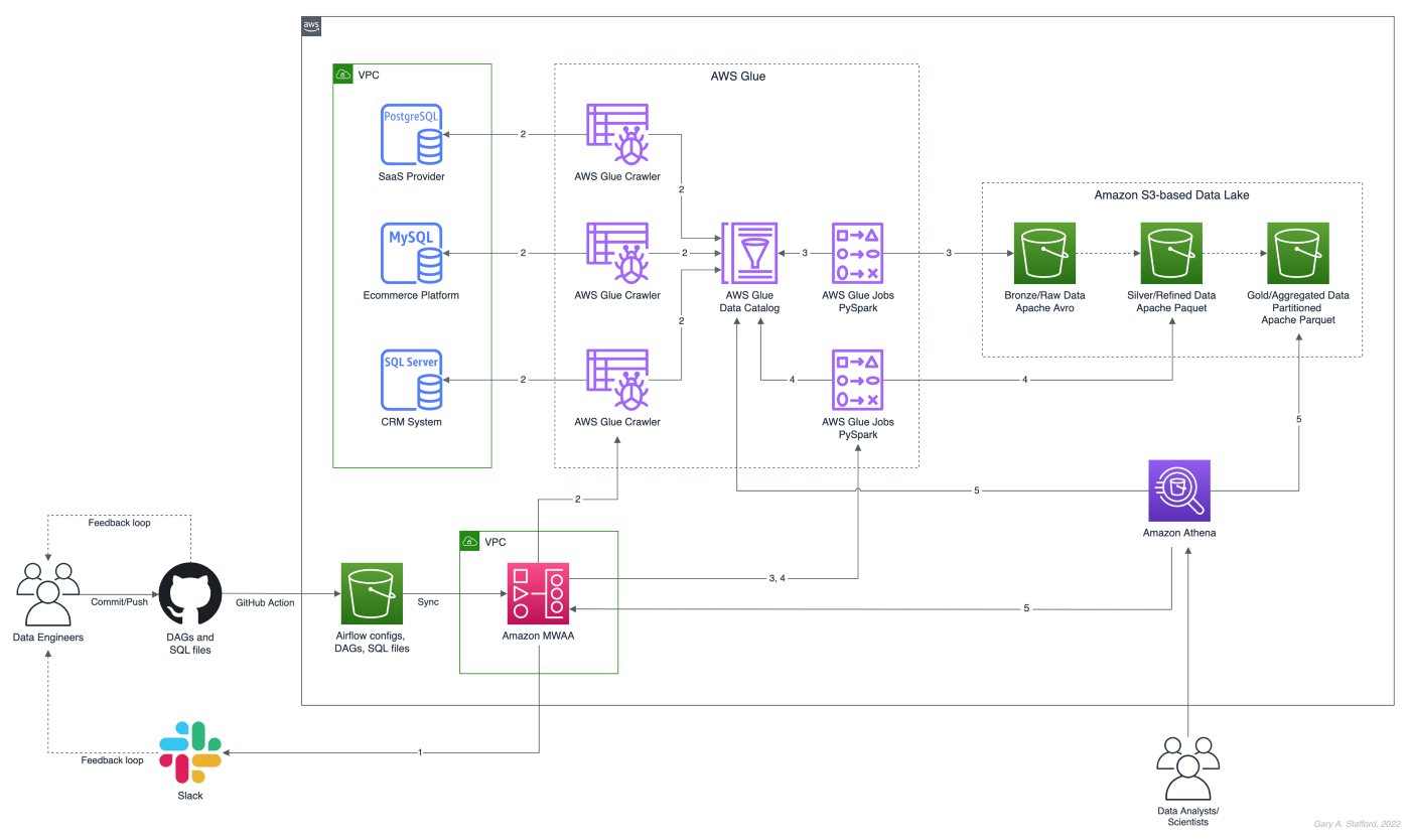
There are endless data sources to build a demonstration data lake on AWS. This post uses the TICKIT sample database provided by AWS and designed for Amazon Redshift, AWS’s cloud data warehousing service. The database consists of seven tables. Two previous posts and associated videos, Building a Data Lake on AWS with Apache Airflow and Building a Data Lake on AWS, detail the setup of the data lake used in this post using AWS Glue and optionally Apache Airflow with Amazon MWAA.
Those two posts use the data lake pattern of segmenting data as bronze (aka raw), silver (aka refined), and gold (aka aggregated), popularized by Databricks. The data lake simulates a typical scenario where data originates from multiple sources, including an e-commerce platform, a CRM system, and a SaaS provider must be aggregated and analyzed.
Spring Projects with IntelliJ IDE
Although not a requirement, I used JetBrains IntelliJ IDEA 2022 (Ultimate Edition) to develop and test the post’s Spring Boot service. Bootstrapping Spring projects with IntelliJ is easy. Developers can quickly create a Spring project using the Spring Initializr plugin bundled with the IntelliJ.

The Spring Initializr plugin’s new project creation wizard is based on start.spring.io. The plugin allows you to quickly select the Spring dependencies you want to incorporate into your project.

Visual Studio Code
There are also several Spring extensions for the popular Visual Studio Code IDE, including Microsoft’s Spring Initializr Java Support extension.

Gradle
This post uses Gradle instead of Maven to develop, test, build, package, and deploy the Spring service. Based on the packages selected in the new project setup shown above, the Spring Initializr plugin’s new project creation wizard creates a build.gradle file. Additional packages, such as Lombak, Micrometer, and Rest Assured, were added separately.
Amazon Corretto
The Spring boot service is developed for and compiled with the most recent version of Amazon Corretto 17. According to AWS, Amazon Corretto is a no-cost, multiplatform, production-ready distribution of the Open Java Development Kit (OpenJDK). Corretto comes with long-term support that includes performance enhancements and security fixes. Corretto is certified as compatible with the Java SE standard and is used internally at Amazon for many production services.
Source Code
Each API endpoint in the Spring Boot RESTful Web Service has a corresponding POJO data model class, service interface and service implementation class, and controller class. In addition, there are also common classes such as configuration, a client factory, and Athena-specific request/response methods. Lastly, there are additional class dependencies for views and prepared statements.

refined_tickit_public_category tableThe project’s source code is arranged in a logical hierarchy by package and class type.
Amazon Athena Access
There are three standard methods for accessing Amazon Athena with the AWS SDK for Java: 1) the AthenaClient service client, 2) the AthenaAsyncClient service client for accessing Athena asynchronously, and 3) using the JDBC driver with the AWS SDK. The AthenaClient and AthenaAsyncClient service clients are both parts of the software.amazon.awssdk.services.athena package. For simplicity, this post’s Spring Boot service uses the AthenaClient service client instead of Java’s asynchronously programming model. AWS supplies basic code samples as part of their documentation as a starting point for writing Athena applications using the SDK. The code samples also use the AthenaClient service client.
POJO-based Data Model Class
For each API endpoint in the Spring Boot RESTful Web Service, there is a corresponding Plain Old Java Object (POJO). According to Wikipedia, a POGO is an ordinary Java object, not bound by any particular restriction. The POJO class is similar to a JPA Entity, representing persistent data stored in a relational database. In this case, the POJO uses Lombok’s @Data annotation. According to the documentation, this annotation generates getters for all fields, a useful toString method, and hashCode and equals implementations that check all non-transient fields. It also generates setters for all non-final fields and a constructor.
Each POJO corresponds directly to a ‘silver’ table in the AWS Glue Data Catalog. For example, the Event POJO corresponds to the refined_tickit_public_event table in the tickit_demo Data Catalog database. The POJO defines the Spring Boot service’s data model for data read from the corresponding AWS Glue Data Catalog table.

The Glue Data Catalog table is the interface between the Athena query and the underlying data stored in Amazon S3 object storage. The Athena query targets the table, which returns the underlying data from S3.

Service Class
Retrieving data from the data lake via AWS Glue, using Athena, is handled by a service class. For each API endpoint in the Spring Boot RESTful Web Service, there is a corresponding Service Interface and implementation class. The service implementation class uses Spring Framework’s @Service annotation. According to the documentation, it indicates that an annotated class is a “Service,” initially defined by Domain-Driven Design (Evans, 2003) as “an operation offered as an interface that stands alone in the model, with no encapsulated state.” Most importantly for the Spring Boot service, this annotation serves as a specialization of @Component, allowing for implementation classes to be autodetected through classpath scanning.
Using Spring’s common constructor-based Dependency Injection (DI) method (aka constructor injection), the service auto-wires an instance of the AthenaClientFactory interface. Note that we are auto-wiring the service interface, not the service implementation, allowing us to wire in a different implementation if desired, such as for testing.
The service calls the AthenaClientFactoryclass’s createClient() method, which returns a connection to Amazon Athena using one of several available authentication methods. The authentication scheme will depend on where the service is deployed and how you want to securely connect to AWS. Some options include environment variables, local AWS profile, EC2 instance profile, or token from the web identity provider.
The service class transforms the payload returned by an instance of GetQueryResultsResponse into an ordered collection (also known as a sequence), List<E>, where E represents a POJO. For example, with the data lake’srefined_tickit_public_event table, the service returns a List<Event>. This pattern repeats itself for tables, views, prepared statements, and named queries. Column data types can be transformed and formatted on the fly, new columns added, and existing columns skipped.
For each endpoint defined in the Controller class, for example, get(), findAll(), and FindById(), there is a corresponding method in the Service class. Below, we see an example of the findAll() method in the SalesByCategoryServiceImp service class. This method corresponds to the identically named method in the SalesByCategoryController controller class. Each of these service methods follows a similar pattern of constructing a dynamic Athena SQL query based on input parameters, which is passed to Athena through the AthenaClient service client using an instance of GetQueryResultsRequest.
Controller Class
Lastly, there is a corresponding Controller class for each API endpoint in the Spring Boot RESTful Web Service. The controller class uses Spring Framework’s @RestController annotation. According to the documentation, this annotation is a convenience annotation that is itself annotated with @Controller and @ResponseBody. Types that carry this annotation are treated as controllers where @RequestMapping methods assume @ResponseBody semantics by default.
The controller class takes a dependency on the corresponding service class application component using constructor-based Dependency Injection (DI). Like the service example above, we are auto-wiring the service interface, not the service implementation.
The controller is responsible for serializing the ordered collection of POJOs into JSON and returning that JSON payload in the body of the HTTP response to the initial HTTP request.
Querying Views
In addition to querying AWS Glue Data Catalog tables (aka Athena tables), we also query views. According to the documentation, a view in Amazon Athena is a logical table, not a physical table. Therefore, the query that defines a view runs each time the view is referenced in a query.
For convenience, each time the Spring Boot service starts, the main AthenaApplication class calls the View.java class’s CreateView() method to check for the existence of the view, view_tickit_sales_by_day_and_category. If the view does not exist, it is created and becomes accessible to all application end-users. The view is queried through the service’s /salesbycategory endpoint.

This confirm-or-create pattern is repeated for the prepared statement in the main AthenaApplication class (detailed in the next section).
Below, we see the View class called by the service at startup.
Aside from the fact the /salesbycategory endpoint queries a view, everything else is identical to querying a table. This endpoint uses the same model-service-controller pattern.
Executing Prepared Statements
According to the documentation, you can use the Athena parameterized query feature to prepare statements for repeated execution of the same query with different query parameters. The prepared statement used by the service, tickit_sales_by_seller, accepts a single parameter, the ID of the seller (sellerid). The prepared statement is executed using the /salesbyseller endpoint. This scenario simulates an end-user of the analytics application who wants to retrieve enriched sales information about their sales.
The pattern of querying data is similar to tables and views, except instead of using the common SELECT...FROM...WHERE SQL query pattern, we use the EXECUTE...USING pattern.
For example, to execute the prepared statement for a seller with an ID of 3, we would use EXECUTE tickit_sales_by_seller USING 3;. We pass the seller’s ID of 3 as a path parameter similar to other endpoints exposed by the service: /v1/salesbyseller/3.

Again, aside from the fact the /salesbyseller endpoint executes a prepared statement and passes a parameter; everything else is identical to querying a table or a view, using the same model-service-controller pattern.
Working with Named Queries
In addition to tables, views, and prepared statements, Athena has the concept of saved queries, referred to as named queries in the Athena API and when using AWS CloudFormation. You can use the Athena console or API to save, edit, run, rename, and delete queries. The queries are persisted using a NamedQueryId, a unique identifier (UUID) of the query. You must reference the NamedQueryId when working with existing named queries.

There are multiple ways to use and reuse existing named queries programmatically. For this demonstration, I created the named query, buyer_likes_by_category, in advance and then stored the resulting NamedQueryId as an application property, injected at runtime or kubernetes deployment time through a local environment variable.
Alternately, you might iterate through a list of named queries to find one that matches the name at startup. However, this method would undoubtedly impact service performance, startup time, and cost. Lastly, you could use a method like NamedQuery() included in the unused NamedQuery class at startup, similar to the view and prepared statement. That named query’s unique NamedQueryId would be persisted as a system property, referencable by the service class. The downside is that you would create a duplicate of the named query each time you start the service. Therefore, this method is also not recommended.
Configuration
Two components responsible for persisting configuration for the Spring Boot service are the application.yml properties file and ConfigProperties class. The class uses Spring Framework’s @ConfigurationProperties annotation. According to the documentation, this annotation is used for externalized configuration. Add this to a class definition or a @Bean method in a @Configuration class if you want to bind and validate some external Properties (e.g., from a .properties or .yml file). Binding is performed by calling setters on the annotated class or, if @ConstructorBinding in use, by binding to the constructor parameters.
The @ConfigurationProperties annotation includes the prefix of athena. This value corresponds to the athena prefix in the the application.yml properties file. The fields in the ConfigProperties class are bound to the properties in the the application.yml. For example, the property, namedQueryId, is bound to the property, athena.named.query.id. Further, that property is bound to an external environment variable, NAMED_QUERY_ID. These values could be supplied from an external configuration system, a Kubernetes secret, or external secrets management system.
AWS IAM: Authentication and Authorization
For the Spring Boot service to interact with Amazon Athena, AWS Glue, and Amazon S3, you need to establish an AWS IAM Role, which the service assumes once authenticated. The Role must be associated with an attached IAM Policy containing the requisite Athena, Glue, and S3 permissions. For development, the service uses a policy similar to the one shown below. Please note this policy is broader than recommended for Production; it does not represent the security best practice of least privilege. In particular, the use of the overly-broad * for Resources should be strictly avoided when creating policies.
In addition to the authorization granted by the IAM Policy, AWS Lake Formation can be used with Amazon S3, AWS Glue, and Amazon Athena to grant fine-grained database-, table-, column-, and row-level access to datasets.
Swagger UI and the OpenAPI Specification
The easiest way to view and experiment with all the endpoints available through the controller classes is using the Swagger UI, included in the example Spring Boot service, by way of the springdoc-openapi Java library. The Swagger UI is accessed at /v1/swagger-ui/index.html.

The OpenAPI Specification (formerly Swagger Specification) is an API description format for REST APIs. The /v1/v3/api-docs endpoint allows you to generate an OpenAPI v3 specification file. The OpenAPI file describes the entire API.

The OpenAPI v3 specification can be saved as a file and imported into applications like Postman, the API platform for building and using APIs.

/users API endpoint using Postman
Integration Tests
Included in the Spring Boot service’s source code is a limited number of example integration tests, not to be confused with unit tests. Each test class uses Spring Framework’s @SpringBootTest annotation. According to the documentation, this annotation can be specified on a test class that runs Spring Boot-based tests. It provides several features over and above the regular Spring TestContext Framework.
The integration tests use Rest Assured’s given-when-then pattern of testing, made popular as part of Behavior-Driven Development (BDD). In addition, each test uses the JUnit’s @Test annotation. According to the documentation, this annotation signals that the annotated method is a test method. Therefore, methods using this annotation must not be private or static and must not return a value.
Run the integration tests using Gradle from the project’s root: ./gradlew clean build test. A detailed ‘Test Summary’ is produced in the project’s build directory as HTML for easy review.


Load Testing the Service
In Production, the Spring Boot service will need to handle multiple concurrent users executing queries against Amazon Athena.

We could use various load testing tools to evaluate the service’s ability to handle multiple concurrent users. One of the simplest is my favorite go-based utility, hey, which sends load to a URL using a provided number of requests in the provided concurrency level and prints stats. It also supports HTTP2 endpoints. So, for example, we could execute 500 HTTP requests with a concurrency level of 25 against the Spring Boot service’s /users endpoint using hey. The post’s integration tests were run against three Kubernetes replica pods of the service deployed to Amazon EKS.
hey -n 500 -c 25 -T "application/json;charset=UTF-8" \
  -h2 https://athena.example-api.com/v1/users

From Athena’s Recent Queries console, we see many simultaneous queries being queued and executed by a hey through the Spring Boot service’s endpoint.

Metrics
The Spring Boot service implements the micrometer-registry-prometheus extension. The Micrometer metrics library exposes runtime and application metrics. Micrometer defines a core library, providing a registration mechanism for metrics and core metric types. These metrics are exposed by the service’s /v1/actuator/prometheus endpoint.

Using the Micrometer extension, metrics exposed by the /v1/actuator/prometheus endpoint can be scraped and visualized by tools such as Prometheus. Conveniently, AWS offers the fully-managed Amazon Managed Service for Prometheus (AMP), which easily integrates with Amazon EKS.

Using Prometheus as a datasource, we can build dashboards in Grafana to observe the service’s metrics. Like AMP, AWS also offers the fully-managed Amazon Managed Grafana (AMG).
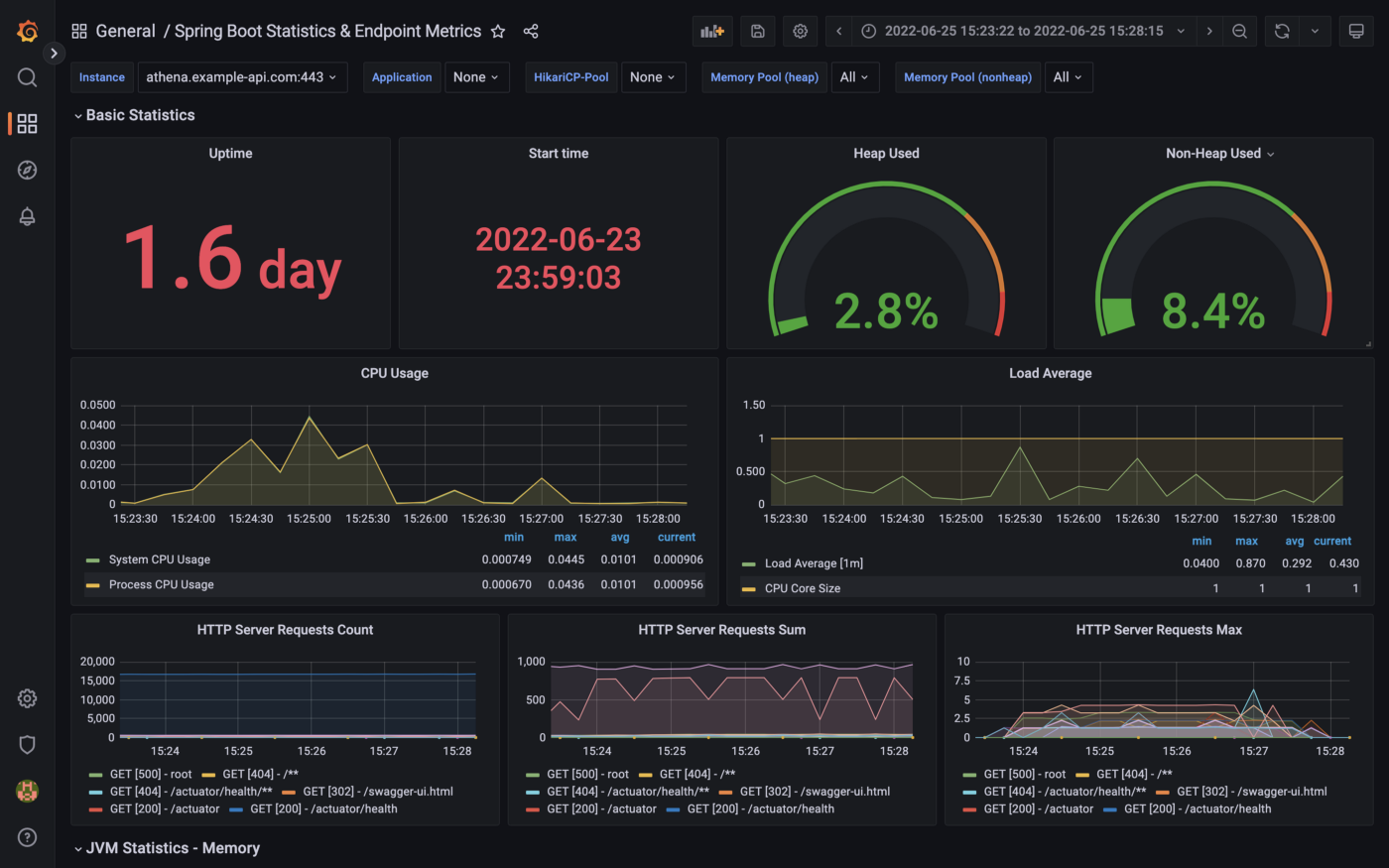

Conclusion
This post taught us how to create a Spring Boot RESTful Web Service, allowing end-user applications to securely query data stored in a data lake on AWS. The service used AWS SDK for Java to access data stored in Amazon S3 through an AWS Glue Data Catalog using Amazon Athena.
This blog represents my own viewpoints and not of my employer, Amazon Web Services (AWS). All product names, logos, and brands are the property of their respective owners. All diagrams and illustrations are property of the author unless otherwise noted.
Building and Deploying Cloud-Native Quarkus-based Java Applications to Kubernetes
Posted by Gary A. Stafford in AWS, Cloud, DevOps, Java Development, Kubernetes, Software Development on June 1, 2022
Developing, testing, building, and deploying Native Quarkus-based Java microservices to Kubernetes on AWS, using GitOps
Introduction
Although it may no longer be the undisputed programming language leader, according to many developer surveys, Java still ranks right up there with Go, Python, C/C++, and JavaScript. Given Java’s continued popularity, especially amongst enterprises, and the simultaneous rise of cloud-native software development, vendors have focused on creating purpose-built, modern JVM-based frameworks, tooling, and standards for developing applications — specifically, microservices.
Leading JVM-based microservice application frameworks typically provide features such as native support for a Reactive programming model, MicroProfile, GraalVM Native Image, OpenAPI and Swagger definition generation, GraphQL, CORS (Cross-Origin Resource Sharing), gRPC (gRPC Remote Procedure Calls), CDI (Contexts and Dependency Injection), service discovery, and distributed tracing.
Leading JVM-based Microservices Frameworks
Review lists of the most popular cloud-native microservices framework for Java, and you are sure to find Spring Boot with Spring Cloud, Micronaut, Helidon, and Quarkus at or near the top.
Spring Boot with Spring Cloud
According to their website, Spring makes programming Java quicker, easier, and safer for everybody. Spring’s focus on speed, simplicity, and productivity has made it the world’s most popular Java framework. Spring Boot makes it easy to create stand-alone, production-grade Spring based Applications that you can just run. Spring Boot’s many purpose-built features make it easy to build and run your microservices in production at scale. However, the distributed nature of microservices brings challenges. Spring Cloud can help with service discovery, load-balancing, circuit-breaking, distributed tracing, and monitoring with several ready-to-run cloud patterns. It can even act as an API gateway.
Helidon
Oracle’s Helidon is a cloud-native, open‑source set of Java libraries for writing microservices that run on a fast web core powered by Netty. Helidon supports MicroProfile, a reactive programming model, and, similar to Micronaut, Spring, and Quarkus, it supports GraalVM Native Image.
Micronaut
According to their website, the Micronaut framework is a modern, open-source, JVM-based, full-stack toolkit for building modular, easily testable microservice and serverless applications. Micronaut supports a polyglot programming model, discovery services, distributed tracing, and aspect-oriented programming (AOP). In addition, Micronaut offers quick startup time, blazing-fast throughput, and a minimal memory footprint.
Quarkus
Quarkus, developed and sponsored by RedHat, is self-described as the ‘Supersonic Subatomic Java.’ Quarkus is a cloud-native, Kubernetes-native, [Linux] container first, microservices first framework for writing Java applications. Quarkus is a Kubernetes Native Java stack tailored for OpenJDK HotSpot and GraalVM, crafted from over fifty best-of-breed Java libraries and standards.
Developing Native Quarkus Microservices
In the following post, we will develop, build, test, deploy, and monitor a native Quarkus microservice application to Kubernetes. The RESTful service will expose a rich Application Programming Interface (API) and interacts with a PostgreSQL database on the backend.
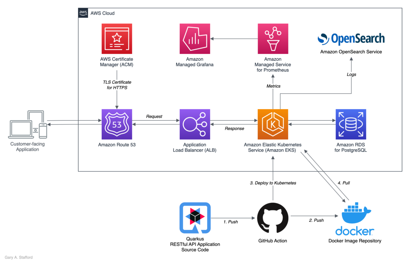
Some of the features of the Quarkus application in this post include:
- Hibernate Object Relational Mapper (ORM), the de facto Jakarta Persistence API (formerly Java Persistence API) implementation
- Hibernate Reactive with Panache, a Quarkus-specific library that simplifies the development of Hibernate Reactive entities
- RESTEasy Reactive, a new JAX-RS implementation, works with the common Vert.x layer and is thus fully reactive
- Advanced RESTEasy Reactive Jackson support for JSON serialization
- Reactive PostgreSQL client
- Built on Mandrel, a downstream distribution of the GraalVM community edition
- Built with Gradle, the modern, open-source build automation tool focused on flexibility and performance
TL;DR
Do you want to explore the source code for this post’s Quarkus microservice application or deploy it to Kubernetes before reading the full article? All the source code and Kubernetes resources are open-source and available on GitHub:
git clone --depth 1 -b main \
    https://github.com/garystafford/tickit-srv.git
The latest Docker Image is available on docker.io:
docker pull garystafford/tickit-srv:<latest-tag>
Quarkus Projects with IntelliJ IDE
Although not a requirement, I used JetBrains IntelliJ IDEA 2022 (Ultimate Edition) to develop and test the post’s Quarkus application. Bootstrapping Quarkus projects with IntelliJ is easy. Using the Quarkus plugin bundled with the Ultimate edition, developers can quickly create a Quarkus project.

The Quarkus plugin’s project creation wizard is based on code.quarkus.io. If you have bootstrapped a Spring Initializr project, code.quarkus.io works very similar to start.spring.io.

Visual Studio Code
RedHat also provides a Quarkus extension for the popular Visual Studio Code IDE.

Gradle
This post uses Gradle instead of Maven to develop, test, build, package, and deploy the Quarkus application to Kubernetes. Based on the packages selected in the new project setup shown above, the Quarkus plugin’s project creation wizard creates the following build.gradle file (Lombak added separately).
The wizard also created the following gradle.properties file, which has been updated to the latest release of Quarkus available at the time of this post, 2.9.2.
Gradle and Quarkus
You can use the Quarkus CLI or the Quarkus Maven plugin to scaffold a Gradle project. Taking a dependency on the Quarkus plugin adds several additional Quarkus tasks to Gradle. We will use Gradle to develop, test, build, containerize, and deploy the Quarkus microservice application to Kubernetes. The quarkusDev, quarkusTest, and quarkusBuild tasks will be particularly useful in this post.

Java Compilation
The Quarkus application in this post is compiled as a native image with the most recent Java 17 version of Mandrel, a downstream distribution of the GraalVM community edition.
GraalVM and Native Image
According to the documentation, GraalVM is a high-performance JDK distribution. It is designed to accelerate the execution of applications written in Java and other JVM languages while also providing runtimes for JavaScript, Ruby, Python, and other popular languages.
Further, according to GraalVM, Native Image is a technology to ahead-of-time compile Java code to a stand-alone executable, called a native image. This executable includes the application classes, classes from its dependencies, runtime library classes, and statically linked native code from the JDK. The Native Image builder (native-image) is a utility that processes all classes of an application and their dependencies, including those from the JDK. It statically analyzes data to determine which classes and methods are reachable during the application execution.
Mandrel
Mandrel is a downstream distribution of the GraalVM community edition. Mandrel’s main goal is to provide a native-image release specifically to support Quarkus. The aim is to align the native-image capabilities from GraalVM with OpenJDK and Red Hat Enterprise Linux libraries to improve maintainability for native Quarkus applications. Mandrel can best be described as a distribution of a regular OpenJDK with a specially packaged GraalVM Native Image builder (native-image).
Docker Image
Once complied, the native Quarkus executable will run within the quarkus-micro-image:1.0 base runtime image deployed to Kubernetes. Quarkus provides this base image to ease the containerization of native executables. It has a minimal footprint (10.9 compressed/29.5 MB uncompressed) compared to other images. For example, the latest UBI (Universal Base Image) Quarkus Mandrel image (ubi-quarkus-mandrel:22.1.0.0-Final-java17) is 714 MB uncompressed, while the OpenJDK 17 image (openjdk:17-jdk) is 471 MB uncompressed. Even RedHat’s Universal Base Image Minimal image (ubi-minimal:8.6) is 93.4 MB uncompressed.

An even smaller option from Quarkus is a distroless base image (quarkus-distroless-image:1.0) is only 9.2 MB compressed / 22.7 MB uncompressed. Quarkus is careful to note that distroless image support is experimental and should not be used in production without rigorous testing.
PostgreSQL Database
For the backend data persistence tier of the Quarkus application, we will use PostgreSQL. All DDL (Data Definition Language) and DML (Data Manipulation Language) statements used in the post were tested with the most current version of PostgreSQL 14.
There are many PostgreSQL-compatible sample databases available that could be used for this post. I am using the TICKIT sample database provided by AWS and designed for Amazon Redshift, AWS’s cloud data warehousing service. The database consists of seven tables — two fact tables and five dimensions tables — in a traditional data warehouse star schema.
For this post, I have remodeled the TICKIT database’s star schema into a normalized relational data model optimized for the Quarkus application. The most significant change to the database is splitting the original Users dimension table into two separate tables — buyer and seller. This change will allow for better separation of concerns (SoC), scalability, and increased protection of Personal Identifiable Information (PII).

Source Code
Each of the six tables in the PostgreSQL TICKIT database is represented by an Entity, Repository, and Resource Java class.

Entity Class
Java Persistence is the API for managing persistence and object/relational mapping. The Java Persistence API (JPA) provides Java developers with an object/relational mapping facility for managing relational data in Java applications. Each table in the PostgreSQL TICKIT database is represented by a Java Persistence Entity, as indicated by the Entity annotation on the class declaration. The annotation specifies that the class is an entity.

Each entity class extends the PanacheEntityBase class, part of the io.quarkus.hibernate.orm.panache package. According to the Quarkus documentation, You can specify your own custom ID strategy, which is done in this post’s example, by extending PanacheEntityBase instead of PanacheEntity.
If you do not want to bother defining getters/setters for your entities, which we did not in the post’s example, extending PanacheEntityBase, Quarkus will generate them for you. Alternately, extend PanacheEntity and take advantage of the default ID it provides if you are not using a custom ID strategy.
The example SaleEntity class shown below is typical of the Quarkus application’s entities. The entity class contains several additional JPA annotations in addition to Entity, including Table, NamedQueries, Id, SequenceGenerator, GeneratedValue, and Column. The entity class also leverages Project Lombok annotations. Lombok generates two boilerplate constructors, one that takes no arguments (NoArgsConstructor) and one that takes one argument for every field (AllArgsConstructor).
The SaleEntity class also defines two many-to-one relationships, with the ListingEntity and BuyerEntity entity classes. This relationship mirrors the database’s data model, as reflected in the schema diagram above. The relationships are defined using the ManyToOne and JoinColumn JPA annotations.
Given the relationships between the entities, a saleEntity object, represented as a nested JSON object, would look as follows:
Repository Class
Each table in the PostgreSQL TICKIT database also has a corresponding repository class, often referred to as the ‘repository pattern.’ The repository class implements the PanacheRepositoryBase interface, part of the io.quarkus.hibernate.orm.panache package. The PanacheRepositoryBase Java interface represents a Repository for a specific type of Entity. According to the documentation, if you are using repositories and have a custom ID strategy, then you will want to extend PanacheRepositoryBase instead of PanacheRepository and specify your ID type as an extra type parameter. Implementing the PanacheRepositoryBase will give you the same methods on the PanacheEntityBase.

The repository class allows us to leverage the methods already available through PanacheEntityBase and add additional custom methods. For example, the repository class contains a custom method listWithPaging. This method retrieves (GET) a list of SaleEntity objects with the added benefit of being able to indicate the page number, page size, sort by field, and sort direction.
Since there is a many-to-one relationship between the SaleEntity class and the ListingEntity and BuyerEntity entity classes, we also have two custom methods that retrieve all SaleEntity objects by either the BuyerEntity ID or the EventEntity ID. These two methods call the SQL queries in the SaleEntity, annotated with the JPA NamedQueries/NamedQuery annotations on the class declaration.
SmallRye Mutiny
Each method defined in the repository class returns a SmallRye Mutiny Uni<T>. According to the website, Mutiny is an intuitive, event-driven Reactive programming library for Java. Mutiny provides a simple but powerful asynchronous development model that lets you build reactive applications. Mutiny can be used in any Java application exhibiting asynchrony, including reactive microservices, data streaming, event processing, API gateways, and network utilities.
Uni
Again, according to Mutiny’s documentation, a Uni represents a stream that can only emit either an item or a failure event. A Uni<T> is a specialized stream that emits only an item or a failure. Typically, Uni<T> are great for representing asynchronous actions such as a remote procedure call, an HTTP request, or an operation producing a single result. A Uni represents a lazy asynchronous action. It follows the subscription pattern, meaning that the action is only triggered once a UniSubscriber subscribes to the Uni.
Resource Class
Lastly, each table in the PostgreSQL TICKIT database has a corresponding resource class. According to the Quarkus documentation, all the operations defined within PanacheEntityBase are available on your repository, so using it is exactly the same as using the active record pattern, except you need to inject it. We inject the corresponding repository class into the resource class, exposing all the available methods of the repository and PanacheRepositoryBase. For example, note the custom listWithPaging method below, which was declared in the SaleRepository class.

Similar to the repository class, each method defined in the resource class also returns a SmallRye Mutiny (io.smallrye.mutiny) Uni<T>.
The repository defines HTTP methods (POST, GET, PUT, and DELETE) corresponding to CRUD operations on the database (Create, Read, Update, and Delete). The methods are annotated with the corresponding javax.ws.rs annotation, indicating the type of HTTP request they respond to. The javax.ws.rs package contains high-level interfaces and annotations used to create RESTful service resources, such as our Quarkus application.
The POST, PUT, and DELETE annotated methods all have the io.quarkus.hibernate.reactive.panache.common.runtime package’s ReactiveTransactional annotation associated with them. We use this annotation on methods to run them in a reactive Mutiny.Session.Transation. If the annotated method returns a Uni, which they do, this has precisely the same behavior as if the method was enclosed in a call to Mutiny.Session.withTransaction(java.util.function.Function). If the method call fails, the complete transaction is rolled back.
Developer Experience
Quarkus has several features to enhance the developer experience. Features include Dev Services, Dev UI, live reload of code without requiring a rebuild and restart of the application, continuous testing where tests run immediately after code changes have been saved, configuration profiles, Hibernate ORM, JUnit, and REST Assured integrations. Using these Quarkus features, it’s easy to develop and test Quarkus applications.
Configuration Profiles
Similar to Spring, Quarkus works with configuration profiles. According to RedHat, you can use different configuration profiles depending on your environment. Configuration profiles enable you to have multiple configurations in the same application.properties file and select between them using a profile name. Quarkus recognizes three default profiles:
- dev: Activated in development mode
- test: Activated when running tests
- prod: The default profile when not running in development or test mode
In the application.properties file, the profile is prefixed using %environment. format. For example, when defining Quarkus’ log level as INFO, you add the common quarkus.log.level=INFO property. However, to change only the test environment’s log level to DEBUG, corresponding to the test profile, you would add a property with the %test. prefix, such as %test.quarkus.log.level=DEBUG.
Dev Services
Quarkus supports the automatic provisioning of unconfigured services in development and test mode, referred to as Dev Services. If you include an extension and do not configure it, then Quarkus will automatically start the relevant service using Test containers behind the scenes and wire up your application to use this service.
When developing your Quarkus application, you could create your own local PostgreSQL database, for example, with Docker:
And the corresponding application configuration properties:
Zero-Config Database
Alternately, we can rely on Dev Services, using a feature referred to as zero config setup. Quarkus provides you with a zero-config database out of the box; no database configuration is required. Quarkus takes care of provisioning the database, running your DDL and DML statements to create database objects and populate the database with test data, and finally, de-provisioning the database container when the development or test session is completed. The database Dev Services will be enabled when a reactive or JDBC datasource extension is present in the application and the database URL has not been configured.
Using the quarkusDev Gradle task, we can start the application running, as shown in the video below. Note the two new Docker containers that are created. Also, note the project’s import.sql SQL script is run automatically, executing all DDL and DML statements to prepare and populate the database.
Bootstrapping the TICKIT Database
When using Hibernate ORM with Quarkus, we have several options regarding how the database is handled when the Quarkus application starts. These are defined in the application.properties file. The quarkus.hibernate-orm.database.generation property determines whether the database schema is generated or not. drop-and-create is ideal in development mode, as shown above. This property defaults to none, however, if Dev Services is in use and no other extensions that manage the schema are present, this will default to drop-and-create. Accepted values: none, create, drop-and-create, drop, update, validate. For development and testing modes, we are using Dev Services with the default value of drop-and-create. For this post, we assume the database and schema already exist in production.
A second property, quarkus.hibernate-orm.sql-load-script, provides the path to a file containing the SQL statements to execute when Hibernate ORM starts. In dev and test modes, it defaults to import.sql. Simply add an import.sql file in the root of your resources directory, Hibernate will be picked up without having to set this property. The project contains an import.sql script to create all database objects and a small amount of test data. You can also explicitly set different files for different profiles and prefix the property with the profile (e.g., %dev. or %test.).
%dev.quarkus.hibernate-orm.database.generation=drop-and-create
%dev.quarkus.hibernate-orm.sql-load-script=import.sql
Another option is Flyway, the popular database migration tool commonly used in JVM environments. Quarkus provides first-class support for using Flyway.
Dev UI
According to the documentation, Quarkus now ships with a new experimental Dev UI, which is available in dev mode (when you start Quarkus with Gradle’s quarkusDev task) at /q/dev by default. It allows you to quickly visualize all the extensions currently loaded, see their status and go directly to their documentation. In addition to access to loaded extensions, you can review logs and run tests in the Dev UI.

Configuration
From the Dev UI, you can access and modify the Quarkus application’s application configuration.

You also can view the configuration of Dev Services, including the running containers and no-config database config.

Quarkus REST Score Console
With RESTEasy Reactive extension loaded, you can access the Quarkus REST Score Console from the Dev UI. The REST Score Console shows endpoint performance through scores and color-coding: green, yellow, or red. RedHat published a recent blog that talks about the scoring process and how to optimize the performance endpoints. Three measurements show whether a REST reactive application can be optimized further.

Application Testing
Quarkus enables robust JVM-based and Native continuous testing by providing integrations with common test frameworks, such as including JUnit, Mockito, and REST Assured. Many of Quarkus’ testing features are enabled through annotations, such as QuarkusTestResource, QuarkusTest, QuarkusIntegrationTest, and TransactionalQuarkusTest.
Quarkus supports the use of mock objects using two different approaches. You can either use CDI alternatives to mock out a bean for all test classes or use QuarkusMock to mock out beans on a per-test basis. This includes integration with Mockito.
The REST Assured integration is particularly useful for testing the Quarkus microservice API application. According to their website, REST Assured is a Java DSL for simplifying testing of REST-based services. It supports the most common HTTP request methods and can be used to validate and verify the response of these requests. REST Assured uses the given(), when(), then() methods of testing made popular as part of Behavior-Driven Development (BDD).
The tests can be run using the the quarkusTest Gradle task. The application contains a small number of integration tests to demonstrate this feature.

Swagger and OpenAPI
Quarkus provides the Smallrye OpenAPI extension compliant with the MicroProfile OpenAPI specification, which allows you to generate an API OpenAPI v3 specification and expose the Swagger UI. The /q/swagger-ui resource exposes the Swagger UI, allowing you to visualize and interact with the Quarkus API’s resources without having any implementation logic in place.

Resources can be tested using the Swagger UI without writing any code.

OpenAPI Specification (formerly Swagger Specification) is an API description format for REST APIs. The /q/openapi resource allows you to generate an OpenAPI v3 specification file. An OpenAPI file allows you to describe your entire API.

The OpenAPI v3 specification can be saved as a file and imported into applications like Postman, the API platform for building and using APIs.


GitOps with GitHub Actions
For this post, GitOps is used to continuously test, build, package, and deploy the Quarkus microservice application to Kubernetes. Specifically, the post uses GitHub Actions. GitHub Actions is a continuous integration and continuous delivery (CI/CD) platform that allows you to automate your build, test, and deployment pipelines. Workflows are defined in the .github/workflows directory in a repository, and a repository can have multiple workflows, each of which can perform a different set of tasks.

Two GitHub Actions are associated with this post’s GitHub repository. The first action, build-test.yml, natively builds and tests the source code in a native Mandrel container on each push to GitHub. The second action (shown below), docker-build-push.yml, builds and containerizes the natively-built executable, pushes it to Docker’s Container Registry (docker.io), and finally deploys the application to Kubernetes. This action is triggered by pushing a new Git Tag to GitHub.

There are several Quarkus configuration properties included in the action’s build step. Alternately, these properties could be defined in the application.properties file. However, I have decided to include them as part of the Gradle build task since they are specific to the type of build and container registry and Kubernetes platform I am pushing to artifacts.
Kubernetes Resources
The Kubernetes resources YAML file, created by the Quarkus build, is also uploaded and saved as an artifact in GitHub by the final step in the GitHub Action.

Quarkus automatically generates ServiceAccount, Role, RoleBinding, Service, Deployment resources.
Choosing a Kubernetes Platform
The only cloud provider-specific code is in the second GitHub action.
In this case, the application is being deployed to an existing Amazon Elastic Kubernetes Service (Amazon EKS), a fully managed, certified Kubernetes conformant service from AWS. These steps can be easily replaced with steps to deploy to other Cloud platforms, such as Microsoft’s Azure Kubernetes Service (AKS) or Google Cloud’s Google Kubernetes Engine (GKE).
GitHub Secrets
Some of the properties use GitHub environment variables, and others use secure GitHub repository encrypted secrets. Secrets are used to secure Docker credentials used to push the Quarkus application image to Docker’s image repository, AWS IAM credentials, and the base64 encoded contents of the kubeconfig file required to deploy to Kubernetes on AWS when using the kodermax/kubectl-aws-eks@master GitHub action.

Docker
Reviewing the configuration properties included in the action’s build step, note the Mandrel container used to build the native Quarkus application, quay.io/quarkus/ubi-quarkus-mandrel:22.1.0.0-Final-java17. Also, note the project’s Docker file is used to build the final Docker image, pushed to the image repository, and then used to provision containers on Kubernetes, src/main/docker/Dockerfile.native-micro. This Dockerfile uses the quay.io/quarkus/quarkus-micro-image:1.0 base image to containerize the native Quarkus application.
The properties also define the image’s repository name and tag (e.g., garystafford/tickit-srv:1.1.0).


Kubernetes
In addition to creating the ticket Namespace in advance, a Kubernetes secret is pre-deployed to the ticket Namespace. The GitHub Action also requires a Role and RoleBinding to deploy the workload to the Kubernetes cluster. Lastly, a HorizontalPodAutoscaler (HPA) is used to automatically scale the workload.
export NAMESPACE=tickit# Namespace
kubectl create namespace ${NAMESPACE}# Role and RoleBinding for GitHub Actions to deploy to Amazon EKS
kubectl apply -f kubernetes/github_actions_role.yml -n ${NAMESPACE}# Secret
kubectl apply -f kubernetes/secret.yml -n ${NAMESPACE}# HorizontalPodAutoscaler (HPA)
kubectl apply -f kubernetes/tickit-srv-hpa.yml -n ${NAMESPACE}
As part of the configuration properties included in the action’s build step, note the use of Kubernetes secrets.
-Dquarkus.kubernetes-config.secrets=tickit
-Dquarkus.kubernetes-config.secrets.enabled=true
This secret contains base64 encoded sensitive credentials and connection values to connect to the Production PostgreSQL database. For this post, I have pre-built an Amazon RDS for PostgreSQL database instance, created the ticket database and required database objects, and lastly, imported the sample data included in the GitHub repository, garystafford/tickit-srv-data.
The five keys seen in the Secret are used in the application.properties file to provide access to the Production PostgreSQL database from the Quakus application.
An even better alternative to using Kubernetes secrets on Amazon EKS is AWS Secrets and Configuration Provider (ASCP) for the Kubernetes Secrets Store CSI Driver. AWS Secrets Manager stores secrets as files mounted in Amazon EKS pods.
AWS Architecture
The GitHub Action pushes the application’s image to Docker’s Container Registry (docker.io), then deploys the application to Kubernetes. Alternately, you could use AWS’s Amazon Elastic Container Registry (Amazon ECR). Amazon EKS pulls the image from Docker as it creates the Kubernetes Pod containers.
There are many ways to route traffic from a requestor to the Quarkus application running on Kubernetes. For this post, the Quarkus application is exposed as a Kubernetes Service on a NodePort. For this post, I have registered a domain, example-api.com, with Amazon Route 53 and a corresponding TLS certificate with AWS Certificate Manager. Inbound requests to the Quarkus application are directed to a subdomain, ticket.example-api.com using HTTPS or port 443. Amazon Route 53 routes those requests to a Layer 7 application load balancer (ALB). The ALB then routes those requests to the Amazon EKS Kubernetes cluster on the NodePort using simple round-robin load balancing. Requests will be routed automatically by Kubernetes to the appropriate worker node and Kubernetes pod. The response then traverses a similar path back to the requestor.
Results
If the GitHub action is successful, any push of code changes to GitHub results in the deployment of the application to Kubernetes.

We can also view the deployed Quarkus application resources using the Kubernetes Dashboard.

Metrics
The post’s Quarkus application implements the micrometer-registry-prometheus extension. The Micrometer metrics library exposes runtime and application metrics. Micrometer defines a core library, providing a registration mechanism for metrics and core metric types.

Using the Micrometer extension, a metrics resource is exposed at /q/metrics, which can be scraped and visualized by tools such as Prometheus. AWS offers its fully-managed Amazon Managed Service for Prometheus (AMP), which easily integrates with Amazon EKS.

Using Prometheus as a datasource, we can build dashboards in Grafana to observe the Quarkus Application metrics. Similar to AMP, AWS offers its fully managed Amazon Managed Grafana (AMG).

Centralized Log Management
According to Quarkus documentation, internally, Quarkus uses JBoss Log Manager and the JBoss Logging facade. You can use the JBoss Logging facade inside your code or any of the supported Logging APIs, including JDK java.util.logging (aka JUL), JBoss Logging, SLF4J, and Apache Commons Logging. Quarkus will send them to JBoss Log Manager.
There are many ways to centralize logs. For example, you can send these logs to open-source centralized log management systems like Graylog, Elastic Stack, fka ELK (Elasticsearch, Logstash, Kibana), EFK (Elasticsearch, Fluentd, Kibana), and OpenSearch with Fluent Bit.
If you are using Kubernetes, the simplest way is to send logs to the console and integrate a central log manager inside your cluster. Since the Quarkus application in this post is running on Amazon EKS, I have chosen Amazon OpenSearch Service with Fluent Bit, an open-source and multi-platform Log Processor and Forwarder. Fluent Bit is fully compatible with Docker and Kubernetes environments. Amazon provides an excellent workshop on installing and configuring Amazon OpenSearch Service with Fluent Bit.


Conclusion
As we learned in this post, Quarkus, the ‘Supersonic Subatomic Java’ framework, is a cloud-native, Kubernetes-native, container first, microservices first framework for writing Java applications. We observed how to build, test, and deploy a RESTful Quarkus Native application to Kubernetes.
Quarkus has capabilities and features well beyond this post’s scope. In a future post, we will explore other abilities of Quarkus, including observability, GraphQL integration, caching, database proxying, tracing and debugging, message queues, data pipelines, and streaming analytics.
This blog represents my own viewpoints and not of my employer, Amazon Web Services (AWS). All product names, logos, and brands are the property of their respective owners. All diagrams and illustrations are property of the author.
Monolith to Microservices: Refactoring Relational Databases
Posted by Gary A. Stafford in Enterprise Software Development, SQL, Technology Consulting on April 14, 2022
Exploring common patterns for refactoring relational database models as part of a microservices architecture
Introduction
There is no shortage of books, articles, tutorials, and presentations on migrating existing monolithic applications to microservices, nor designing new applications using a microservices architecture. It has been one of the most popular IT topics for the last several years. Unfortunately, monolithic architectures often have equally monolithic database models. As organizations evolve from monolithic to microservices architectures, refactoring the application’s database model is often overlooked or deprioritized. Similarly, as organizations develop new microservices-based applications, they frequently neglect to apply a similar strategy to their databases.

The following post will examine several basic patterns for refactoring relational databases for microservices-based applications.
Terminology
Monolithic Architecture
A monolithic architecture is “the traditional unified model for the design of a software program. Monolithic, in this context, means composed all in one piece.” (TechTarget). A monolithic application “has all or most of its functionality within a single process or container, and it’s componentized in internal layers or libraries” (Microsoft). A monolith is usually built, deployed, and upgraded as a single unit of code.
Microservices Architecture
A microservices architecture (aka microservices) refers to “an architectural style for developing applications. Microservices allow a large application to be separated into smaller independent parts, with each part having its own realm of responsibility” (Google Cloud).
According to microservices.io, the advantages of microservices include:
- Highly maintainable and testable
- Loosely coupled
- Independently deployable
- Organized around business capabilities
- Owned by a small team
- Enables rapid, frequent, and reliable delivery
- Allows an organization to [more easily] evolve its technology stack
Database
A database is “an organized collection of structured information, or data, typically stored electronically in a computer system” (Oracle). There are many types of databases. The most common database engines include relational, NoSQL, key-value, document, in-memory, graph, time series, wide column, and ledger.
PostgreSQL
In this post, we will use PostgreSQL (aka Postgres), a popular open-source object-relational database. A relational database is “a collection of data items with pre-defined relationships between them. These items are organized as a set of tables with columns and rows. Tables are used to hold information about the objects to be represented in the database” (AWS).
Amazon RDS for PostgreSQL
We will use the fully managed Amazon RDS for PostgreSQL in this post. Amazon RDS makes it easy to set up, operate, and scale PostgreSQL deployments in the cloud. With Amazon RDS, you can deploy scalable PostgreSQL deployments in minutes with cost-efficient and resizable hardware capacity. In addition, Amazon RDS offers multiple versions of PostgreSQL, including the latest version used for this post, 14.2.
The patterns discussed here are not specific to Amazon RDS for PostgreSQL. There are many options for using PostgreSQL on the public cloud or within your private data center. Alternately, you could choose Amazon Aurora PostgreSQL-Compatible Edition, Google Cloud’s Cloud SQL for PostgreSQL, Microsoft’s Azure Database for PostgreSQL, ElephantSQL, or your own self-manage PostgreSQL deployed to bare metal servers, virtual machine (VM), or container.
Database Refactoring Patterns
There are many ways in which a relational database, such as PostgreSQL, can be refactored to optimize efficiency in microservices-based application architectures. As stated earlier, a database is an organized collection of structured data. Therefore, most refactoring patterns reorganize the data to optimize for an organization’s functional requirements, such as database access efficiency, performance, resilience, security, compliance, and manageability.
The basic building block of Amazon RDS is the DB instance, where you create your databases. You choose the engine-specific characteristics of the DB instance when you create it, such as storage capacity, CPU, memory, and EC2 instance type on which the database server runs. A single Amazon RDS database instance can contain multiple databases. Those databases contain numerous object types, including tables, views, functions, procedures, and types. Tables and other object types are organized into schemas. These hierarchal constructs — instances, databases, schemas, and tables — can be arranged in different ways depending on the requirements of the database data producers and consumers.

Sample Database
To demonstrate different patterns, we need data. Specifically, we need a database with data. Conveniently, due to the popularity of PostgreSQL, there are many available sample databases, including the Pagila database. I have used it in many previous articles and demonstrations. The Pagila database is available for download from several sources.

The Pagila database represents a DVD rental business. The database is well-built, small, and adheres to a third normal form (3NF) database schema design. The Pagila database has many objects, including 1 schema, 15 tables, 1 trigger, 7 views, 8 functions, 1 domain, 1 type, 1 aggregate, and 13 sequences. Pagila’s tables contain between 2 and 16K rows.
Pattern 1: Single Schema
Pattern 1: Single Schema is one of the most basic database patterns. There is one database instance containing a single database. That database has a single schema containing all tables and other database objects.

As organizations begin to move from monolithic to microservices architectures, they often retain their monolithic database architecture for some time.

Frequently, the monolithic database’s data model is equally monolithic, lacking proper separation of concerns using simple database constructs such as schemas. The Pagila database is an example of this first pattern. The Pagila database has a single schema containing all database object types, including tables, functions, views, procedures, sequences, and triggers.
To create a copy of the Pagila database, we can use pg_restore to restore any of several publically available custom-format database archive files. If you already have the Pagila database running, simply create a copy with pg_dump.
Below we see the table layout of the Pagila database, which contains the single, default public schema.
-----------+----------+--------+------------
 Instance  | Database | Schema | Table
-----------+----------+--------+------------
 postgres1 | pagila   | public | actor
 postgres1 | pagila   | public | address
 postgres1 | pagila   | public | category
 postgres1 | pagila   | public | city
 postgres1 | pagila   | public | country
 postgres1 | pagila   | public | customer
 postgres1 | pagila   | public | film
 postgres1 | pagila   | public | film_actor
 postgres1 | pagila   | public | film_category
 postgres1 | pagila   | public | inventory
 postgres1 | pagila   | public | language
 postgres1 | pagila   | public | payment
 postgres1 | pagila   | public | rental
 postgres1 | pagila   | public | staff
 postgres1 | pagila   | public | store
Using a single schema to house all tables, especially the public schema is generally considered poor database design. As a database grows in complexity, creating, organizing, managing, and securing dozens, hundreds, or thousands of database objects, including tables, within a single schema becomes impossible. For example, given a single schema, the only way to organize large numbers of database objects is by using lengthy and cryptic naming conventions.
Public Schema
According to the PostgreSQL docs, if tables or other object types are created without specifying a schema name, they are automatically assigned to the default public schema. Every new database contains a public schema. By default, users cannot access any objects in schemas they do not own. To allow that, the schema owner must grant the USAGE privilege on the schema. by default, everyone has CREATE and USAGE privileges on the schema public. These default privileges enable all users to connect to a given database to create objects in its public schema. Some usage patterns call for revoking that privilege, which is a compelling reason not to use the public schema as part of your database design.
Pattern 2: Multiple Schemas
Separating tables and other database objects into multiple schemas is an excellent first step to refactoring a database to support microservices. As application complexity and databases naturally grow over time, schemas to separate functionality by business subdomain or teams will benefit significantly.
According to the PostgreSQL docs, there are several reasons why one might want to use schemas:
- To allow many users to use one database without interfering with each other.
- To organize database objects into logical groups to make them more manageable.
- Third-party applications can be put into separate schemas, so they do not collide with the names of other objects.
Schemas are analogous to directories at the operating system level, except schemas cannot be nested.

With Pattern 2, as an organization continues to decompose its monolithic application architecture to a microservices-based application, it could transition to a schema-per-microservice or similar level or organizational granularity.

Applying Domain-driven Design Principles
Domain-driven design (DDD) is “a software design approach focusing on modeling software to match a domain according to input from that domain’s experts” (Wikipedia). Architects often apply DDD principles to decompose a monolithic application into microservices. For example, a microservice or set of related microservices might represent a Bounded Context. In DDD, a Bounded Context is “a description of a boundary, typically a subsystem or the work of a particular team, within which a particular model is defined and applicable.” (hackernoon.com). Examples of Bounded Context might include Sales, Shipping, and Support.
One technique to apply schemas when refactoring a database is to mirror the Bounded Contexts, which reflect the microservices. For each microservice or set of closely related microservices, there is a schema. Unfortunately, there is no absolute way to define the Bounded Contexts of a Domain, and henceforth, schemas to a database. It depends on many factors, including your application architecture, features, security requirements, and often an organization’s functional team structure.
Reviewing the purpose of each table in the Pagila database and their relationships to each other, we could infer Bounded Contexts, such as Films, Stores, Customers, and Sales. We can represent these Bounded Contexts as schemas within the database as a way to organize the data. The individual tables in a schema mirror DDD concepts, such as aggregates, entities, or value objects.
As shown below, the tables of the Pagila database have been relocated into six new schemas: common, customers, films, sales, staff, and stores. The common schema contains tables with address data references tables in several other schemas. There are now no tables left in the public schema. We will assume other database objects (e.g., functions, views, and triggers) have also been moved and modified if necessary to reflect new table locations.
-----------+----------+-----------+---------------
 Instance  | Database | Schema    | Table
-----------+----------+-----------+---------------
 postgres1 | pagila   | common    | address
 postgres1 | pagila   | common    | city
 postgres1 | pagila   | common    | country
-----------+----------+-----------+---------------
 postgres1 | pagila   | customers | customer
-----------+----------+-----------+---------------
 postgres1 | pagila   | films     | actor
 postgres1 | pagila   | films     | category
 postgres1 | pagila   | films     | film
 postgres1 | pagila   | films     | film_actor
 postgres1 | pagila   | films     | film_category
 postgres1 | pagila   | films     | language
-----------+----------+-----------+---------------
 postgres1 | pagila   | sales     | payment
 postgres1 | pagila   | sales     | rental
-----------+----------+-----------+---------------
 postgres1 | pagila   | staff     | staff
-----------+----------+-----------+---------------
 postgres1 | pagila   | stores    | inventory
 postgres1 | pagila   | stores    | store
By applying schemas, we align tables and other database objects to individual microservices or functional teams that own the microservices and the associated data. Schemas allow us to apply fine-grain access control over objects and data within the database more effectively.

Refactoring other Database Objects
Typically with psql, when moving tables across schemas using an ALTER TABLE...SET SCHEMA... SQL statement, objects such as database views will be updated to the table’s new location. For example, take Pagila’s sales_by_store view. Note the schemas have been automatically updated for multiple tables from their original location in the public schema. The view was also moved to the sales schema.
Splitting Table Data Across Multiple Schemas
When refactoring a database, you may have to split data by replicating table definitions across multiple schemas. Take, for example, Pagila’s address table, which contains the addresses of customers, staff, and stores. The customers.customer, stores.staff, and stores.store all have foreign key relationships with the common.address table. The address table has a foreign key relationship with both the city and country tables. Thus for convenience, the address, city, and country tables were all placed into the common schema in the example above.
Although, at first, storing all the addresses in a single table might appear to be sound database normalization, consider the risks of having the address table’s data exposed. The store addresses are not considered sensitive data. However, the home addresses of customers and staff are likely considered sensitive personally identifiable information (PII). Also, consider as an application evolves, you may have fields unique to one type of address that does not apply to other categories of addresses. The table definitions for a store’s address may be defined differently than the address of a customer. For example, we might choose to add a county column to the customers.address table for e-commerce tax purposes, or an on_site_parking boolean column to the stores.address table.
In the example below, a new staff schema was added. The address table definition was replicated in the customers, staff, and stores schemas. The assumption is that the mixed address data in the original table was distributed to the appropriate address tables. Note the way schemas help us avoid table name collisions.
-----------+----------+-----------+---------------
 Instance  | Database | Schema    | Table
-----------+----------+-----------+---------------
 postgres1 | pagila   | common    | city
 postgres1 | pagila   | common    | country
-----------+----------+-----------+---------------
 postgres1 | pagila   | customers | address
 postgres1 | pagila   | customers | customer
-----------+----------+-----------+---------------
 postgres1 | pagila   | films     | actor
 postgres1 | pagila   | films     | category
 postgres1 | pagila   | films     | film
 postgres1 | pagila   | films     | film_actor
 postgres1 | pagila   | films     | film_category
 postgres1 | pagila   | films     | language
-----------+----------+-----------+---------------
 postgres1 | pagila   | sales     | payment
 postgres1 | pagila   | sales     | rental
-----------+----------+-----------+---------------
 postgres1 | pagila   | staff     | address
 postgres1 | pagila   | staff     | staff
-----------+----------+-----------+---------------
 postgres1 | pagila   | stores    | address
 postgres1 | pagila   | stores    | inventory
 postgres1 | pagila   | stores    | store
To create the new customers.address table, we could use the following SQL statements. The statements to create the other two address tables are nearly identical.
Although we now have two additional tables with identical table definitions, we do not duplicate any data. We could use the following SQL statements to migrate unique address data into the appropriate tables and confirm the results.
Lastly, alter the existing foreign key constraints to point to the new address tables. The SQL statements for the other two address tables are nearly identical.
There is now a reduced risk of exposing sensitive customer or staff data when querying store addresses, and the three address entities can evolve independently. Individual functional teams separately responsible customers, staff, and stores, can own and manage just the data within their domain.
Before dropping the common.address tables, you would still need to modify the remaining database objects that have dependencies on this table, such as views and functions. For example, take Pagila’s sales_by_store view we saw previously. Note line 9, below, the schema of the address table has been updated from common.address to stores.address. The stores.address table only contains addresses of stores, not customers or staff.
Below, we see the final table structure for the Pagila database after refactoring. Tables have been loosely grouped together schema in the diagram.
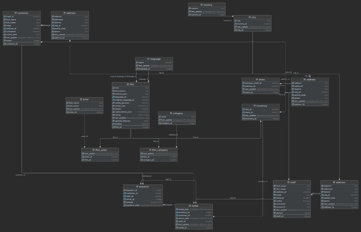
Pattern 3: Multiple Databases
Similar to how individual schemas allow us to organize tables and other database objects and provide better separation of concerns, we can use databases the same way. For example, we could choose to spread the Pagila data across more than one database within a single RDS database instance. Again, using DDD concepts, while schemas might represent Bounded Contexts, databases most closely align to Domains, which are “spheres of knowledge and activity where the application logic revolves” (hackernoon.com).

With Pattern 3, as an organization continues to refine its microservices-based application architecture, it might find that multiple databases within the same database instance are advantageous to further separate and organize application data.

Let’s assume that the data in the films schema is owned and managed by a completely separate team who should never have access to sensitive data stored in the customers, stores, and sales schemas. According to the PostgreSQL docs, database access permissions are managed using the concept of roles. Depending on how the role is set up, a role can be thought of as either a database user or a group of users.
To provide greater separation of concerns than just schemas, we can create a second, completely separate database within the same RDS database instance for data related to films. With two separate databases, it is easier to create and manage distinct roles and ensure access to customers, stores, or sales data is only accessible to teams that need access.
Below, we see the new layout of tables now spread across two databases within the same RDS database instance. Two new tables, highlighted in bold, are explained below.
-----------+----------+-----------+---------------
 Instance  | Database | Schema    | Table
-----------+----------+-----------+---------------
 postgres1 | pagila   | common    | city
 postgres1 | pagila   | common    | country
-----------+----------+-----------+---------------
 postgres1 | pagila   | customers | address
 postgres1 | pagila   | customers | customer
-----------+----------+-----------+---------------
 postgres1 | pagila   | films     | film
-----------+----------+-----------+---------------
 postgres1 | pagila   | sales     | payment
 postgres1 | pagila   | sales     | rental
-----------+----------+-----------+---------------
 postgres1 | pagila   | staff     | address
 postgres1 | pagila   | staff     | staff
-----------+----------+-----------+---------------
 postgres1 | pagila   | stores    | address
 postgres1 | pagila   | stores    | inventory
 postgres1 | pagila   | stores    | store
-----------+----------+-----------+---------------
 postgres1 | products | films     | actor
 postgres1 | products | films     | category
 postgres1 | products | films     | film
 postgres1 | products | films     | film_actor
 postgres1 | products | films     | film_category
 postgres1 | products | films     | language
 postgres1 | products | films     | outbox
Change Data Capture and the Outbox Pattern
Inserts, updates, and deletes of film data can be replicated between the two databases using several methods, including Change Data Capture (CDC) with the Outbox Pattern. CDC is “a pattern that enables database changes to be monitored and propagated to downstream systems” (RedHat). The Outbox Pattern uses the PostgreSQL database’s ability to perform an commit to two tables atomically using a transaction. Transactions bundles multiple steps into a single, all-or-nothing operation.
In this example, data is written to existing tables in the products.films schema (updated aggregate’s state) as well as a new products.films.outbox table (new domain events), wrapped in a transaction. Using CDC, the domain events from the products.films.outbox table are replicated to the pagila.films.film table. The replication of data between the two databases using CDC is also referred to as eventual consistency.

In this example, films in the pagila.films.film and products.films.outbox tables are represented in a denormalized, aggregated view of a film instead of the original, normalized relational multi-table structure. The table definition of the new pagila.films.film table is very different than that of the original Pagila products.films.films table. A concept such as a film, represented as an aggregate or entity, can be common to multiple Bounded Contexts, yet have a different definition.
Note the Confluent JDBC Source Connector (io.confluent.connect.jdbc.JdbcSourceConnector) used here will not work with PostgreSQL arrays, which would be ideal for one-to-many categories and actors columns. Arrays can be converted to text using ::text or by building value-delimited strings using string_agg aggregate function.
Given this table definition, the resulting data would look as follows.
The existing pagila.stores.inventory table has a foreign key constraint on the the pagila.films.film table. However, the films schema and associated tables have been migrated to the products database’s films schema. To overcome this challenge, we can:
- Create a new
pagila.films.filmtable - Continuously replicate data from the
productsdatabase to thepagila.films.filmtable data using CDC (see below) - Modify the
pagila.stores.inventorytable to take a dependency on the newfilmtable - Drop the duplicate tables and other objects from the
pagila.filmsschema
Debezium and Confluent for CDC
There are several technology choices for performing CDC. For this post, I have used RedHat’s Debezium connector for PostgreSQL and Debezium Outbox Event Router, and Confluent’s JDBC Sink Connector. Below, we see a typical example of a Kafka Connect Source Connector using the Debezium connector for PostgreSQL and a Sink Connector using the Confluent JDBC Sink Connector. The Source Connector streams changes from the products logs, using PostgreSQL’s Write-Ahead Logging (WAL) feature, to an Apache Kafka topic. A corresponding Sink Connector streams the changes from the Kafka topic to the pagila database.
Pattern 4: Multiple Database Instances
At some point in the evolution of a microservices-based application, it might become advantageous to separate the data into multiple database instances using the same database engine. Although managing numerous database instances may require more resources, there are also advantages. Each database instance will have independent connection configurations, roles, and administrators. Each database instance could run different versions of the database engine, and each could be upgraded and maintained independently.

With Pattern 4, as an organization continues to refine its application architecture, it might find that multiple database instances are beneficial to further separate and organize application data.

Below is one possible refactoring of the Pagila database, splitting the data between two database engines. The first database instance, postgres1, contains two databases, pagila and products. The second database instance, postgres2, contains a single database, products.
-----------+----------+-----------+---------------
 Instance  | Database | Schema    | Table
-----------+----------+-----------+---------------
 postgres1 | pagila   | common    | city
 postgres1 | pagila   | common    | country
-----------+----------+-----------+---------------
 postgres1 | pagila   | customers | address
 postgres1 | pagila   | customers | customer
-----------+----------+-----------+---------------
 postgres1 | pagila   | films     | actor
 postgres1 | pagila   | films     | category
 postgres1 | pagila   | films     | film
 postgres1 | pagila   | films     | film_actor
 postgres1 | pagila   | films     | film_category
 postgres1 | pagila   | films     | language
-----------+----------+-----------+---------------
 postgres1 | pagila   | staff     | address
 postgres1 | pagila   | staff     | staff
-----------+----------+-----------+---------------
 postgres1 | pagila   | stores    | address
 postgres1 | pagila   | stores    | inventory
 postgres1 | pagila   | stores    | store
-----------+----------+-----------+---------------
 postgres1 | pagila   | sales     | payment
 postgres1 | pagila   | sales     | rental
-----------+----------+-----------+---------------
 postgres2 | products | films     | actor
 postgres2 | products | films     | category
 postgres2 | products | films     | film
 postgres2 | products | films     | film_actor
 postgres2 | products | films     | film_category
 postgres2 | products | films     | language
Data Replication with CDC
Note the films schema is duplicated between the two databases, shown above. Again, using the CDC allows us to keep the six postgres1.pagila.films tables in sync with the six postgres2.products.films tables using CDC. In this example, we are not using the OutBox Pattern, as used previously in Pattern 3. Instead, we are replicating any changes to any of the tables in postgres2.products.films schema to the corresponding tables in the postgres1.pagila.films schema.

To ensure the tables stay in sync, the tables and other objects in the postgres1.pagila.films schema should be limited to read-only access (SELECT) for all users. The postgres2.products.films tables represent the authoritative source of data, the System of Record (SoR). Any inserts, updates, or deletes, must be made to these tables and replicated using CDC.
Pattern 5: Multiple Database Engines
AWS commonly uses the term ‘purpose-built databases.’ AWS offers over fifteen purpose-built database engines to support diverse data models, including relational, key-value, document, in-memory, graph, time series, wide column, and ledger. There may be instances where using multiple, purpose-built databases makes sense. Using different database engines allows architects to take advantage of the unique characteristics of each engine type to support diverse application requirements.
With Pattern 5, as an organization continues to refine its application architecture, it might choose to leverage multiple, different database engines.

Take for example an application that uses a combination of relational, NoSQL, and in-memory databases to persist data. In addition to PostgreSQL, the application benefits from moving a certain subset of its relational data to a non-relational, high-performance key-value store, such as Amazon DynamoDB. Furthermore, the application implements a database cache using an ultra-fast in-memory database, such as Amazon ElastiCache for Redis.
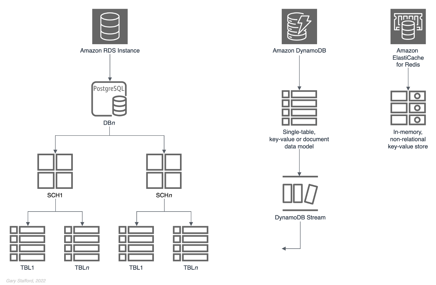
Below is one possible refactoring of the Pagila database, splitting the data between two different database engines, PostgreSQL and Amazon DynamoDB.
-----------+----------+-----------+-----------
 Instance  | Database | Schema    | Table
-----------+----------+-----------+-----------
 postgres1 | pagila   | common    | city
 postgres1 | pagila   | common    | country
-----------+----------+-----------+-----------
 postgres1 | pagila   | customers | address
 postgres1 | pagila   | customers | customer
-----------+----------+-----------+-----------
 postgres1 | pagila   | films     | film
-----------+----------+-----------+-----------
 postgres1 | sales    | sales     | payment
 postgres1 | sales    | sales     | rental
-----------+----------+-----------+-----------
 postgres1 | pagila   | staff     | address
 postgres1 | pagila   | staff     | staff
-----------+----------+-----------+-----------
 postgres1 | pagila   | stores    | address
 postgres1 | pagila   | stores    | film
 postgres1 | pagila   | stores    | inventory
 postgres1 | pagila   | stores    | store
-----------+----------+-----------+-----------
 DynamoDB  |    -     |     -     | Films
The assumption is that based on the application’s access patterns for film data, the application could benefit from the addition of a non-relational, high-performance key-value store. Further, the film-related data entities, such as a film , category, and actor, could be modeled using DynamoDB’s single-table data model architecture. In this model, multiple entity types can be stored in the same table. If necessary, to replicate data back to the PostgreSQL instance from the DynamoBD instance, we can perform CDC with DynamoDB Streams.

Films data model for DynamoDB using NoSQL Workbench
Films data modelCQRS
Command Query Responsibility Segregation (CQRS), a popular software architectural pattern, is another use case for multiple database engines. The CQRS pattern is, as the name implies, “a software design pattern that separates command activities from query activities. In CQRS parlance, a command writes data to a data source. A query reads data from a data source. CQRS addresses the problem of data access performance degradation when applications running at web-scale have too much burden placed on the physical database and the network on which it resides” (RedHat). CQRS commonly uses one database engine optimized for writes and a separate database optimized for reads.

Conclusion
Embracing a microservices-based application architecture may have many business advantages for an organization. However, ignoring the application’s existing databases can negate many of the benefits of microservices. This post examined several common patterns for refactoring relational databases to match a modern microservices-based application architecture.
This blog represents my own viewpoints and not of my employer, Amazon Web Services (AWS). All product names, logos, and brands are the property of their respective owners. All diagrams and illustrations are property of the author.
End-to-End Data Discovery, Observability, and Governance on AWS with LinkedIn’s Open-source DataHub
Posted by Gary A. Stafford in Analytics, AWS, Azure, Bash Scripting, Build Automation, Cloud, DevOps, GCP, Kubernetes, Python, Software Development, SQL, Technology Consulting on March 26, 2022
Use DataHub’s data catalog capabilities to collect, organize, enrich, and search for metadata across multiple platforms
Introduction
According to Shirshanka Das, Founder of LinkedIn DataHub, Apache Gobblin, and Acryl Data, one of the simplest definitions for a data catalog can be found on the Oracle website: “Simply put, a data catalog is an organized inventory of data assets in the organization. It uses metadata to help organizations manage their data. It also helps data professionals collect, organize, access, and enrich metadata to support data discovery and governance.”
Another succinct description of a data catalog’s purpose comes from Alation: “a collection of metadata, combined with data management and search tools, that helps analysts and other data users to find the data that they need, serves as an inventory of available data, and provides information to evaluate the fitness of data for intended uses.”
Working with many organizations in the area of Analytics, one of the more common requests I receive regards choosing and implementing a data catalog. Organizations have datasources hosted in corporate data centers, on AWS, by SaaS providers, and with other Cloud Service Providers. Several of these organizations have recently gravitated to DataHub, the open-source metadata platform for the modern data stack, originally developed by LinkedIn.

In this post, we will explore the capabilities of DataHub to build a centralized data catalog on AWS for datasources hosted in multiple AWS accounts, SaaS providers, cloud service providers, and corporate data centers. I will demonstrate how to build a DataHub data catalog using out-of-the-box data source plugins for automated metadata ingestion.
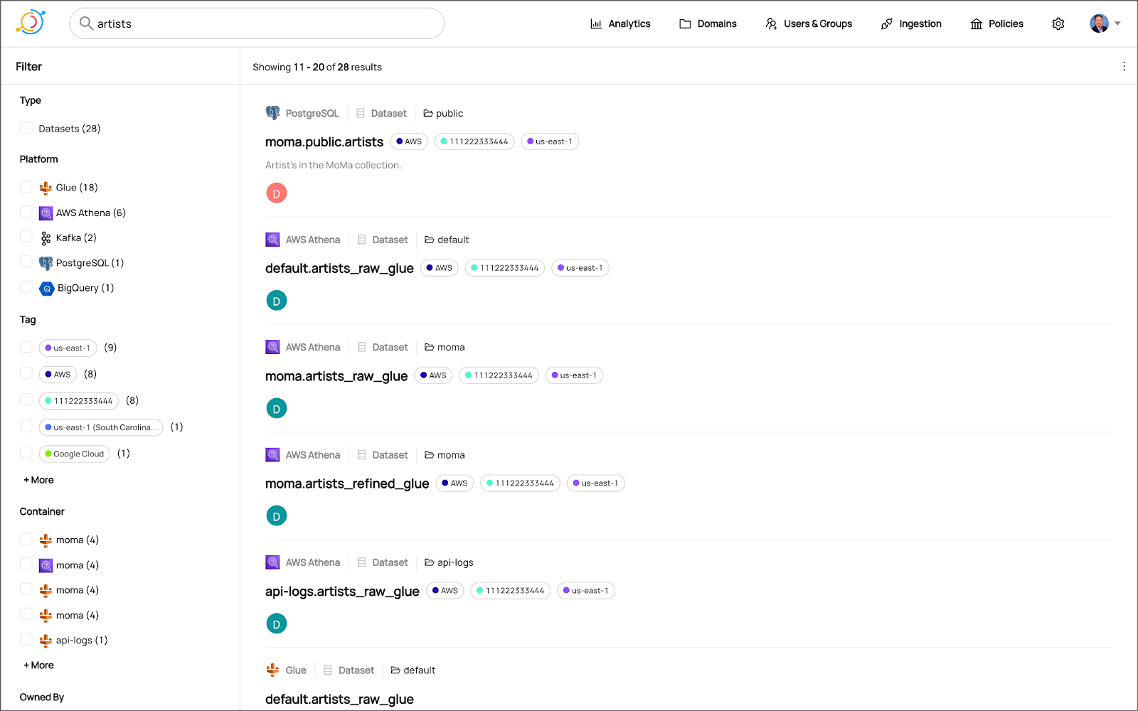
Data Catalog Competitors
Data catalogs are not new; technologies such as data dictionaries have been around as far back as the 1980’s. Gartner publishes their Metadata Management (EMM) Solutions Reviews and Ratings and Metadata Management Magic Quadrant. These reports contain a comprehensive list of traditional commercial enterprise players, modern cloud-native SaaS vendors, and Cloud Service Provider (CSP) offerings. DBMS Tools also hosts a comprehensive list of 30 data catalogs. A sampling of current data catalogs includes:
Open Source Software
Commercial
- Acryl Data (based on LinkedIn’s DataHub)
- Atlan
- Stemma (based on Lyft’s Amundsen)
- Talend
- Alation
- Collibra
- data.world
Cloud Service Providers
Data Catalog Features
DataHub describes itself as “a modern data catalog built to enable end-to-end data discovery, data observability, and data governance.” Sorting through vendor’s marketing jargon and hype, standard features of leading data catalogs include:
- Metadata ingestion
- Data discovery
- Data governance
- Data observability
- Data lineage
- Data dictionary
- Data classification
- Usage/popularity statistics
- Sensitive data handling
- Data fitness (aka data quality or data profiling)
- Manage both technical and business metadata
- Business glossary
- Tagging
- Natively supported datasource integrations
- Advanced metadata search
- Fine-grain authentication and authorization
- UI- and API-based interaction
Datasources
When considering a data catalog solution, in my experience, the most common datasources that customers want to discover, inventory, and search include:
- Relational databases and other OLTP datasources such as PostgreSQL, MySQL, Microsoft SQL Server, and Oracle
- Cloud Data Warehouses and other OLAP datasources such as Amazon Redshift, Snowflake, and Google BigQuery
- NoSQL datasources such as MongoDB, MongoDB Atlas, and Azure Cosmos DB
- Persistent event-streaming platforms such as Apache Kafka (Amazon MSK and Confluent)
- Distributed storage datasets (e.g., Data Lakes) such as Amazon S3, Apache Hive, and AWS Glue Data Catalogs
- Business Intelligence (BI), dashboards, and data visualization sources such as Looker, Tableau, and Microsoft Power BI
- ETL sources, such as Apache Spark, Apache Airflow, Apache NiFi, and dbt
DataHub on AWS
DataHub’s convenient AWS setup guide covers options to deploy DataHub to AWS. For this post, I have hosted DataHub on Kubernetes, using Amazon Elastic Kubernetes Service (Amazon EKS). Alternately, you could choose Google Kubernetes Engine (GKE) on Google Cloud or Azure Kubernetes Service (AKS) on Microsoft Azure.
Conveniently, DataHub offers a Helm chart, making deployment to Kubernetes straightforward. Furthermore, Helm charts are easily integrated with popular CI/CD tools. For this post, I’ve used ArgoCD, the declarative GitOps continuous delivery tool for Kubernetes, to deploy the DataHub Helm charts to Amazon EKS.

According to the documentation, DataHub consists of four main components: GMS, MAE Consumer (optional), MCE Consumer (optional), and Frontend. Kubernetes deployment for each of the components is defined as sub-charts under the main DataHub Helm chart.
External Storage Layer Dependencies
Four external storage layer dependencies power the main DataHub components: Kafka, Local DB (MySQL, Postgres, or MariaDB), Search Index (Elasticsearch), and Graph Index (Neo4j or Elasticsearch). DataHub has provided a separate DataHub Prerequisites Helm chart for the dependencies. The dependencies must be deployed before deploying DataHub.
Alternately, you can substitute AWS managed services for the external storage layer dependencies, which is also detailed in the Deploying to AWS documentation. AWS managed service dependency substitutions include Amazon RDS for MySQL, Amazon OpenSearch (fka Amazon Elasticsearch), and Amazon Managed Streaming for Apache Kafka (Amazon MSK). According to DataHub, support for using AWS Neptune as the Graph Index is coming soon.
DataHub CLI and Plug-ins
DataHub comes with the datahub CLI, allowing you to perform many common operations on the command line. You can install and use the DataHub CLI within your development environment or integrate it with your CI/CD tooling.

DataHub uses a plugin architecture. Plugins allow you to install only the datasource dependencies you need. For example, if you want to ingest metadata from Amazon Athena, just install the Athena plugin: pip install 'acryl-datahub[athena]'. DataHub Source, Sink, and Transformer plugins can be displayed using the datahub check plugins CLI command.


Secure Metadata Ingestion
Often, datasources are not externally accessible for security reasons. Further, many datasources may not be accessible to individual users, especially in higher environments like UAT, Staging, and Production. They are only accessible to applications or CI/CD tooling. To overcome these limitations when extracting metadata with DataHub, I prefer to perform my DataHub-related development and testing locally but execute all DataHub ingestion securely on AWS.
In my local development environment, I use JetBrains PyCharm to author the Python and YAML-based DataHub configuration files and ingestion pipeline recipes, then commit those files to git and push them to a private GitHub repository. Finally, I use GitHub Actions to test DataHub files.
To run DataHub ingestion jobs and push the results to DataHub running in Kubernetes on Amazon EKS, I have built a custom Python-based Docker container. The container runs the DataHub CLI, required DataHub plugins, and any additional Python dependencies. The container’s pod has the appropriate AWS IAM permissions, using IAM Roles for Service Accounts (IRSA), to securely access datasources to ingest and the DataHub application.
Schedule and Monitor Pipelines
Scheduling and managing multiple metadata ingestion jobs on AWS is best handled with Apache Airflow with Amazon Managed Workflows for Apache Airflow (Amazon MWAA). Ingestion jobs run as Airflow DAG tasks, which call the EKS-based DataHub CLI container. With MWAA, datasource connections, credentials, and other sensitive configurations can be kept secure and not be exposed externally or in plain text.
When running the ingestion pipelines on AWS with DataHub, all communications between AWS-based datasources, ingestion jobs running in Airflow, and DataHub, should use secure private IP addressing and DNS resolution instead of transferring metadata over the Internet. Make sure to create all the necessary VPC peering connections, network route table configurations, and VPC endpoints to connect all relevant services.
SaaS services such as Snowflake or MongoDB Atlas, services provided by other Cloud Service Providers such as Google Cloud and Microsoft Azure, and datasources in corporate datasources require alternate networking and security strategies to access metadata securely.

Markup or Code?
According to the documentation, a DataHub recipe is a configuration file that tells ingestion scripts where to pull data from (source) and where to put it (sink). Recipes normally contain a source, sink, and transformers configuration section. Mark-up language-based job automation written in YAML, JSON, or Domain Specific Languages (DSLs) is often an alternative to writing code. DataHub recipes can be written in YAML. The example recipe shown below is used to ingest metadata from an Amazon RDS for PostgreSQL database, running on AWS.
YAML-based recipes can also use automatic environment variable expansion for convenience, automation, and security. It is considered best practice to secure sensitive configuration values, such as database credentials, in a secure location and reference them as environment variables. For example, note the server: ${DATAHUB_REST_ENDPOINT} entry in the sink section below. The DATAHUB_REST_ENDPOINT environment variable is set ahead of time and re-used for all ingestion jobs. Sensitive database connection information has also been variablized and stored separately.
Using Python
You can configure and run a pipeline entirely from within a custom Python script using DataHub’s Python API as an alternative to YAML. Below, we see two nearly identical ingestion recipes to the YAML above, written in Python. Writing ingestion pipeline logic programmatically gives you increased flexibility for automation, error checking, unit-testing, and notification. Below is a basic pipeline written in Python. The code is functional, but not very Pythonic, secure, scalable, or Production ready.
The second version of the same pipeline is more Production ready. The code is more Pythonic in nature and makes use of error checking, logging, and the AWS Systems Manager (SSM) Parameter Store. Like recipes written in YAML, environment variables can be used for convenience and security. In this example, commonly reused and sensitive connection configuration items have been extracted and placed in the SSM Parameter Store. Additional configuration is pulled from the environment, such as AWS Account ID and AWS Region. The script loads these values at runtime.
Sinking to DataHub
When syncing metadata to DataHub, you have two choices, the GMS REST API or Kafka. According to DataHub, the advantage of the REST-based interface is that any errors can immediately be reported. On the other hand, the advantage of the Kafka-based interface is that it is asynchronous and can handle higher throughput. For this post, I am DataHub’s REST API.


Column-level Metadata
In addition to column names and data types, it is possible to extract column descriptions and key types from certain datasources. Column descriptions, tags, and glossary terms can also be input through the DataHub UI. Below, we see an example of an Amazon Redshift fact table, whose table and column descriptions were ingested as part of the metadata.

Business Glossary
DataHub can assign business glossary terms to entities. The DataHub Business Glossary plugin pulls business glossary metadata from a YAML-based configuration file.
Business glossary terms can be reviewed in the Glossary Terms tab of the DataHub’s UI. Below, we see the three terms associated with the Classification glossary node: Confidential, HighlyConfidential, and Sensitive.

We can search for entities inventoried in DataHub using their assigned business glossary terms.

Finally, we see an example of an AWS Athena data catalog table with business glossary terms applied to columns within the table’s schema.

SQL-based Profiler
DataHub also can extract statistics about entities in DataHub using the SQL-based Profiler. According to the DataHub documentation, the Profiler can extract the following:
- Row and column counts for each table
- Column null counts and proportions
- Column distinct counts and proportions
- Column min, max, mean, median, standard deviation, quantile values
- Column histograms or frequencies of unique values
In addition, we can also track the historical stats for each profiled entity each time metadata is ingested.


Data Lineage
DataHub’s data lineage features allow us to view upstream and downstream relationships between different types of entities. DataHub can trace lineage across multiple platforms, datasets, pipelines, charts, and dashboards.
Below, we see a simple example of dataset entity-to-entity lineage in Amazon Redshift and then Apache Spark on Amazon EMR. The fact table has a downstream relationship to four database views. The views are based on SQL queries that include the upstream table as a datasource.


DataHub Analytics
DataHub provides basic metadata quality and usage analytics in the DataHub UI: user activity, counts of datasource types, business glossary terms, environments, and actions.


Conclusion
In this post, we explored the features of a data catalog and learned about some of the leading commercial and open-source data catalogs. Next, we learned how DataHub could collect, organize, enrich, and search metadata across multiple datasources. Lastly, we discovered how easy it is to catalog metadata from datasources spread across multiple CSP, SaaS providers, and corporate data centers, and centralize those results in DataHub.
In addition to the basic features reviewed in this post, DataHub offers a growing number of additional capabilities, including GraphQL and Timeline APIs, robust authentication and authorization, application monitoring observability, and Great Expectations integration. All these qualities make DataHub an excellent choice for a data catalog.
This blog represents my own viewpoints and not of my employer, Amazon Web Services (AWS). All product names, logos, and brands are the property of their respective owners.
Data Preparation on AWS: Comparing Available ELT Options to Cleanse and Normalize Data
Posted by Gary A. Stafford in Analytics, AWS, Build Automation, Cloud, Python, SQL, Technology Consulting on March 1, 2022
Comparing the features and performance of different AWS analytics services for Extract, Load, Transform (ELT)
Introduction
According to Wikipedia, “Extract, load, transform (ELT) is an alternative to extract, transform, load (ETL) used with data lake implementations. In contrast to ETL, in ELT models the data is not transformed on entry to the data lake but stored in its original raw format. This enables faster loading times. However, ELT requires sufficient processing power within the data processing engine to carry out the transformation on demand, to return the results in a timely manner.”
As capital investments and customer demand continue to drive the growth of the cloud-based analytics market, the choice of tools seems endless, and that can be a problem. Customers face a constant barrage of commercial and open-source tools for their batch, streaming, and interactive exploratory data analytics needs. The major Cloud Service Providers (CSPs) have even grown to a point where they now offer multiple services to accomplish similar analytics tasks.
This post will examine the choice of analytics services available on AWS capable of performing ELT. Specifically, this post will compare the features and performance of AWS Glue Studio, Amazon Glue DataBrew, Amazon Athena, and Amazon EMR using multiple ELT use cases and service configurations.
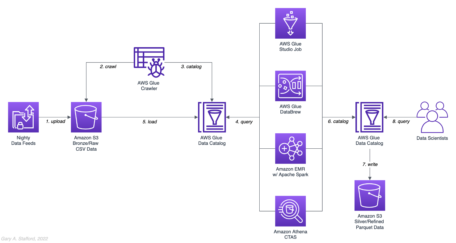
Analytics Use Case
We will address a simple yet common analytics challenge for this comparison — preparing a nightly data feed for analysis the next day. Each night a batch of approximately 1.2 GB of raw CSV-format healthcare data will be exported from a Patient Administration System (PAS) and uploaded to Amazon S3. The data must be cleansed, deduplicated, refined, normalized, and made available to the Data Science team the following morning. The team of Data Scientists will perform complex data analytics on the data and build machine learning models designed for early disease detection and prevention.
Sample Dataset
The dataset used for this comparison is generated by Synthea, an open-source patient population simulation. The high-quality, synthetic, realistic patient data and associated health records cover every aspect of healthcare. The dataset contains the patient-related healthcare history for allergies, care plans, conditions, devices, encounters, imaging studies, immunizations, medications, observations, organizations, patients, payers, procedures, providers, and supplies.
The Synthea dataset was first introduced in my March 2021 post examining the handling of sensitive PII data using Amazon Macie: Data Lakes: Discovery, Security, and Privacy of Sensitive Data.
The Synthea synthetic patient data is available in different record volumes and various data formats, including HL7 FHIR, C-CDA, and CSV. We will use CSV-format data files for this post. Since this post seeks to measure the performance of different AWS ELT-capable services, we will use a larger version of the Synthea dataset containing hundreds of thousands to millions of records.
AWS Glue Data Catalog
The dataset comprises nine uncompressed CSV files uploaded to Amazon S3 and cataloged to an AWS Glue Data Catalog, a persistent metadata store, using an AWS Glue Crawler.

Test Cases
We will use three data preparation test cases based on the Synthea dataset to examine the different AWS ELT-capable services.

Test Case 1: Encounters for Symptom
An encounter is a health care contact between the patient and the provider responsible for diagnosing and treating the patient. In our first test case, we will process 1.26M encounters records for an ongoing study of patient symptoms by our Data Science team.
Data preparation includes the following steps:
- Load 1.26M encounter records using the existing AWS Glue Data Catalog table.
- Remove any duplicate records.
- Select only the records where the
descriptioncolumn contains “Encounter for symptom.” - Remove any rows with an empty
reasoncodescolumn. - Extract a new
year,month, anddaycolumn from thedatecolumn. - Remove the
datecolumn. - Write resulting dataset back to Amazon S3 as Snappy-compressed Apache Parquet files, partitioned by
year,month, andday. - Given the small resultset, bucket the data such that only one file is written per
daypartition to minimize the impact of too many small files on future query performance. - Catalog resulting dataset to a new table in the existing AWS Glue Data Catalog, including partitions.
Test Case 2: Observations
Clinical observations ensure that treatment plans are up-to-date and correctly administered and allow healthcare staff to carry out timely and regular bedside assessments. We will process 5.38M encounters records for our Data Science team in our second test case.
Data preparation includes the following steps:
- Load 5.38M observation records using the existing AWS Glue Data Catalog table.
- Remove any duplicate records.
- Extract a new
year,month, anddaycolumn from the date column. - Remove the
datecolumn. - Write resulting dataset back to Amazon S3 as Snappy-compressed Apache Parquet files, partitioned by
year,month, andday. - Given the small resultset, bucket the data such that only one file is written per
daypartition to minimize the impact of too many small files on future query performance. - Catalog resulting dataset to a new table in the existing AWS Glue Data Catalog, including partitions.
Test Case 3: Sinusitis Study
A medical condition is a broad term that includes all diseases, lesions, and disorders. In our second test case, we will join the conditions records with the patient records and filter for any condition containing the term ‘sinusitis’ in preparation for our Data Science team.
Data preparation includes the following steps:
- Load 483k condition records using the existing AWS Glue Data Catalog table.
- Inner join the condition records with the 132k patient records based on patient ID.
- Remove any duplicate records.
- Drop approximately 15 unneeded columns.
- Select only the records where the
descriptioncolumn contains the term “sinusitis.” - Remove any rows with empty
ethnicity,race,gender, ormaritalcolumns. - Create a new column,
condition_age, based on a calculation of the age in days at which the patient’s condition was diagnosed. - Write the resulting dataset back to Amazon S3 as Snappy-compressed Apache Parquet-format files. No partitions are necessary.
- Given the small resultset, bucket the data such that only one file is written to minimize the impact of too many small files on future query performance.
- Catalog resulting dataset to a new table in the existing AWS Glue Data Catalog.
AWS ELT Options
There are numerous options on AWS to handle the batch transformation use case described above; a non-exhaustive list includes:
- AWS Glue Studio (UI-driven with AWS Glue PySpark Extensions)
- Amazon Glue DataBrew
- Amazon Athena
- Amazon EMR with Apache Spark
- AWS Glue Studio (Apache Spark script)
- AWS Glue Jobs (Legacy jobs)
- Amazon EMR with Presto
- Amazon EMR with Trino
- Amazon EMR with Hive
- AWS Step Functions and AWS Lambda
- Amazon Redshift Spectrum
- Partner solutions on AWS, such as Databricks, Snowflake, Upsolver, StreamSets, Stitch, and Fivetran
- Self-managed custom solutions using a combination of OSS, such as dbt, Airbyte, Dagster, Meltano, Apache NiFi, Apache Drill, Apache Beam, Pandas, Apache Airflow, and Kubernetes
For this comparison, we will choose the first five options listed above to develop our ELT data preparation pipelines: AWS Glue Studio (UI-driven job creation with AWS Glue PySpark Extensions), Amazon Glue DataBrew, Amazon Athena, Amazon EMR with Apache Spark, and AWS Glue Studio (Apache Spark script).
AWS Glue Studio
According to the documentation, “AWS Glue Studio is a new graphical interface that makes it easy to create, run, and monitor extract, transform, and load (ETL) jobs in AWS Glue. You can visually compose data transformation workflows and seamlessly run them on AWS Glue’s Apache Spark-based serverless ETL engine. You can inspect the schema and data results in each step of the job.”
AWS Glue Studio’s visual job creation capability uses the AWS Glue PySpark Extensions, an extension of the PySpark Python dialect for scripting ETL jobs. The extensions provide easier integration with AWS Glue Data Catalog and other AWS-managed data services. As opposed to using the graphical interface for creating jobs with AWS Glue PySpark Extensions, you can also run your Spark scripts with AWS Glue Studio. In fact, we can use the exact same scripts run on Amazon EMR.
For the tests, we are using the G.2X worker type, Glue version 3.0 (Spark 3.1.1 and Python 3.7), and Python as the language choice for this comparison. We will test three worker configurations using both UI-driven job creation with AWS Glue PySpark Extensions and Apache Spark script options:
- 10 workers with a maximum of 20 DPUs
- 20 workers with a maximum of 40 DPUs
- 40 workers with a maximum of 80 DPUs


AWS Glue DataBrew
According to the documentation, “AWS Glue DataBrew is a visual data preparation tool that enables users to clean and normalize data without writing any code. Using DataBrew helps reduce the time it takes to prepare data for analytics and machine learning (ML) by up to 80 percent, compared to custom-developed data preparation. You can choose from over 250 ready-made transformations to automate data preparation tasks, such as filtering anomalies, converting data to standard formats, and correcting invalid values.”
DataBrew allows you to set the maximum number of DataBrew nodes that can be allocated when a job runs. For this comparison, we will test three different node configurations:
- 3 maximum nodes
- 10 maximum nodes
- 20 maximum nodes


Amazon Athena
According to the documentation, “Athena helps you analyze unstructured, semi-structured, and structured data stored in Amazon S3. Examples include CSV, JSON, or columnar data formats such as Apache Parquet and Apache ORC. You can use Athena to run ad-hoc queries using ANSI SQL, without the need to aggregate or load the data into Athena.”
Although Athena is classified as an ad-hoc query engine, using a CREATE TABLE AS SELECT (CTAS) query, we can create a new table in the AWS Glue Data Catalog and write to Amazon S3 from the results of a SELECT statement from another query. That other query statement performs a transformation on the data using SQL.
Amazon Athena is a fully managed AWS service and has no performance settings to adjust or monitor.


CTAS and Partitions
A notable limitation of Amazon Athena for the batch use case is the 100 partition limit with CTAS queries. Athena [only] supports writing to 100 unique partition and bucket combinations with CTAS. Partitioned by year, month, and day, the observations test case requires 2,558 partitions, and the observations test case requires 10,433 partitions. There is a recommended workaround using an INSERT INTO statement. However, the workaround requires additional SQL logic, computation, and most important cost. It is not practical, in my opinion, compared to other methods when a higher number of partitions are needed. To avoid the partition limit with CTAS, we will only partition by year and bucket by month when using Athena. Take this limitation into account when comparing the final results.
Amazon EMR with Apache Spark
According to the documentation, “Amazon EMR is a cloud big data platform for running large-scale distributed data processing jobs, interactive SQL queries, and machine learning (ML) applications using open-source analytics frameworks such as Apache Spark, Apache Hive, and Presto. You can quickly and easily create managed Spark clusters from the AWS Management Console, AWS CLI, or the Amazon EMR API.”
For this comparison, we are using two different Spark 3.1.2 EMR clusters:
- (1) r5.xlarge Master node and (2) r5.2xlarge Core nodes
- (1) r5.2xlarge Master node and (4) r5.2xlarge Core nodes
All Spark jobs are written in both Python (PySpark) and Scala. We are using the AWS Glue Data Catalog as the metastore for Spark SQL instead of Apache Hive.


Results
Data pipelines were developed and tested for each of the three test cases using the five chosen AWS ELT services and configuration variations. Each pipeline was then run 3–5 times, for a total of approximately 150 runs. The resulting AWS Glue Data Catalog table and data in Amazon S3 were deleted between each pipeline run. Each new run created a new data catalog table and wrote new results to Amazon S3. The median execution times from these tests are shown below.


Although we can make some general observations about the execution times of the chosen AWS services, the results are not meant to be a definitive guide to performance. An accurate comparison would require a deeper understanding of how each of these managed services works under the hood, in order to both optimize and balance their compute profiles correctly.
Amazon Athena
The Resultset column contains the final number of records written to Amazon S3 by Athena. The results contain the data pipeline’s median execution time and any additional data points.

AWS Glue Studio (AWS Glue PySpark Extensions)
Tests were run with three different configurations for AWS Glue Studio using the graphical interface for creating jobs with AWS Glue PySpark Extensions. Times for each configuration were nearly identical.

AWS Glue Studio (Apache PySpark script)
As opposed to using the graphical interface for creating jobs with AWS Glue PySpark Extensions, you can also run your Apache Spark scripts with AWS Glue Studio. The tests were run with the same three configurations as above. The execution times compared to the Amazon EMR tests, below, are almost identical.

Amazon EMR with Apache Spark
Tests were run with three different configurations for Amazon EMR with Apache Spark using PySpark. The first set of results is for the 2-node EMR cluster. The second set of results is for the 4-node cluster. The third set of results is for the same 4-node cluster in which the data was not bucketed into a single file within each partition. Compare the execution times and the number of objects against the previous set of results. Too many small files can negatively impact query performance.

It is commonly stated that “Scala is almost ten times faster than Python.” However, with Amazon EMR, jobs written in Python (PySpark) and Scala had similar execution times for all three test cases.

Amazon Glue DataBrew
Tests were run with three different configurations Amazon Glue DataBrew, including 3, 10, and 20 maximum nodes. Times for each configuration were nearly identical.

Observations
- All tested AWS services can read and write to an AWS Glue Data Catalog and the underlying datastore, Amazon S3. In addition, they all work with the most common analytics data file formats.
- All tested AWS services have rich APIs providing access through the AWS CLI and SDKs, which support multiple programming languages.
- Overall, AWS Glue Studio, using the AWS Glue PySpark Extensions, appears to be the most capable ELT tool of the five services tested and with the best performance.
- Both AWS Glue DataBrew and AWS Glue Studio are no-code or low-code services, democratizing access to data for non-programmers. Conversely, Amazon Athena requires knowledge of ANSI SQL, and Amazon EMR with Apache Spark requires knowledge of Scala or Python. Be cognizant of the potential trade-offs from using no-code or low-code services on observability, configuration control, and automation.
- Both AWS Glue DataBrew and AWS Glue Studio can write a custom Parquet writer type optimized for Dynamic Frames, GlueParquet. One potential advantage, a pre-computed schema is not required before writing.
- There is a slight ‘cold-start’ with Glue Studio. Studio startup times ranged from 7 seconds to 2 minutes and 4 seconds in the tests. However, the lower execution time of AWS Glue Studio compared to Amazon EMR with Spark and AWS Glue DataBrew in the tests offsets any initial cold-start time, in my opinion.
- Changing the maximum number of units from 3 to 10 to 20 for AWS Glue DataBrew made negligible differences in job execution times. Given the nearly identical execution times, it is unclear exactly how many units are being used by the job. More importantly, how many DataBrew node hours we are being billed for. These are some of the trade-offs with a fully-managed service — visibility and fine-tuning configuration.
- Similarly, with AWS Glue Studio, using either 10 workers w/ max. 20 DPUs, 20 workers w/ max. 40 DPUs, or 40 workers w/ max. 80 DPUs resulted in nearly identical executions times.
- Amazon Athena had the fastest execution times but is limited by the 100 partition limit for large CTAS resultsets. Athena is not practical, in my opinion, compared to other ELT methods, when a higher number of partitions are needed.
- It is commonly stated that “Scala is almost ten times faster than Python.” However, with Amazon EMR, jobs written in Python (PySpark) and Scala had almost identical execution times for all three test cases.
- Using Amazon EMR with EC2 instances takes about 9 minutes to provision a new cluster for this comparison fully. Given nearly identical execution times to AWS Glue Studio with Apache Spark scripts, Glue has the clear advantage of nearly instantaneous startup times.
- AWS recently announced Amazon EMR Serverless. Although this service is still in Preview, this new version of EMR could potentially reduce or eliminate the lengthy startup time for ephemeral clusters requirements.
- Although not discussed, scheduling the data pipelines to run each night was a requirement for our use case. AWS Glue Studio jobs and AWS Glue DataBrew jobs are schedulable from those services. For Amazon EMR and Amazon Athena, we could use Amazon Managed Workflows for Apache Airflow (MWAA), AWS Data Pipeline, or AWS Step Functions combined with Amazon CloudWatch Events Rules to schedule the data pipelines.
Conclusion
Customers have many options for ELT — the cleansing, deduplication, refinement, and normalization of raw data. We examined chosen services on AWS, each capable of handling the analytics use case presented. The best choice of tools depends on your specific ELT use case and performance requirements.
This blog represents my own viewpoints and not of my employer, Amazon Web Services (AWS). All product names, logos, and brands are the property of their respective owners.
Considerations for Architecting Resilient Multi-Region Workloads
Posted by Gary A. Stafford in Enterprise Software Development, Technology Consulting on January 24, 2022
What to consider when evaluating a ‘multi-region’ strategy as part of business continuity and disaster recovery planning
Introduction
Increasingly, I hear the term ‘multi-region’ used within the IT community and in conversations with peers and customers, most often within the context of disaster recovery. In my experience, ‘multi-region’ is a cloud provider-agnostic phrase that can mean different things to different organizations. A few examples:
- Multiple, independent, regionally-deployed application instances that better serve a geographically-diverse customer base, for regulated ‘locality-restricted’ workloads, to ensure data sovereignty, distribute system load, or minimize the blast radius of a regional disaster event. Although a disaster recovery plan may be required, the primary driver of this architecture is often not disaster recovery.
- An active-passive failover strategy in which a second DR Region hosts a mixture of cold, warm, and hot copies of workloads and serves as a failover in response to a disaster event in the Primary Region. In my experience, this is probably the most common use case when someone refers to ‘multi-region.’
- An active-active architecture in which data is continually replicated and traffic can be seamlessly routed based on geolocation between all services within two or more geo-redundant regions, making it resilient to the impact of a regional disaster event. Some might describe this architecture as having both inner-regional and inter-regional high availability.

Terminology
The following terminology is commonly used when discussing Business Continuity and Disaster Recovery Planning. Teams should be familiar with these concepts before undertaking planning activities:
- Fault Tolerance (FT), High Availability (HA), Disaster Recovery (DR), and Business Continuity (BC), and the distinct differences between the four concepts
- Business Continuity Plan/Planning (BCP) and Disaster Recovery Plan/Planning (DRP), and the differences between the two types of plans (source)
- Business Continuity and Disaster Recovery (BCDR or BC/DR) (source)
- Business Impact Analysis (BIA) and Risk Assessment (source)
- Categories of Disaster: Natural Disasters, Technical Failures, and Human Actions, both intentional and unintentional (source)
- Resiliency, which includes both Disaster Recovery (service restoration) and Availability (preventing loss of service) (source)
- Crisis Management: Critical vs. Non-Critical Systems and Mission Critical vs. Business Critical Systems (source)
- Regions vs. Availability Zones (aka Zones), common constructs to all major Cloud Service Providers (CSP): AWS, Google Cloud, Microsoft Azure, IBM Cloud, and Oracle Cloud
- Primary (aka Active) Region vs. DR (aka Passive or Standby) Region (source)
- Active-Active vs. Active-Passive DR Strategies (source)
- SHARE’s 7 Tiers of Disaster Recovery (source)
- Disaster Recovery Site Types: Cold, Warm, and Hot (source)
- AWS Multi-Region Disaster Recovery Strategies: 1) Backup and restore, 2) active-passive Pilot light, 3) active-passive Warm standby, or 4) Multi-region (multi-site) active-active (source)
- Recovery Time Objective (RTO) and Recovery Point Objective (RPO), and the methods and costs to achieve varying levels of each SLA (source)
- Failover and Failback Operations (source)
- Partial vs. Complete Regional Outage, and the implications to Disaster Recovery Planning (source)
- Single Points of Failure (SPOF) (source)
BCDR Planning Considerations
When developing BCDR Plans that include multi-region, there are several technical aspects of your workloads that need to be considered. The following list is not designed to be exhaustive, nor is it intended to suggest that multi-region DR is an unattainable task. On the contrary, this list is meant to encourage thorough planning and suggest ways to continually improve an organization’s plan.
- Configuration Data Management
- Secret Management
- Cryptographic Key Management
- Hardware Security Module (HSM)
- Credential Management
- SSL/TLS Certificate Management
- Authentication (AuthN) and Authorization (AuthZ)
- Domain Name System (DNS), DNS Failover and Failback, Global Traffic Management (GTM)
- Content delivery network (CDN)
- Specialized Workloads, such as SAP, VMware, SharePoint, Citrix, Oracle, SQL Server, SAP HANA, and IBM Db2
- On-premises workload dependencies, and wide-area network (WAN) connectivity between on-premises data centers and the Cloud
- Remote access from on-premises and remote employees to cloud-based backend and enterprise systems
- Edge compute, such as connected devices, IoT, storage gateways, and remotely-managed local cloud-infrastructure (e.g., AWS Outposts
- DevOps, CI/CD, Release Management
- Infrastructure as Code (IaC)
- Public and private artifact repositories, including Docker and Virtual Machine (VM) Image repositories
- Source code in Version Control Systems (VCS), also known as Source Control Management (SCM)
- Software licensing for the self-managed and hosted services
- Observability, monitoring, logging, alerting, and notification
- Regional differences of a Cloud Provider’s service offerings, cost, performance, and support
- Latency, including latency between Primary and DR Region and between end-users and partners and DR Region
- Data residency and data sovereignty requirements, which will impact choice of DR Region
- Automated, event-driven Failover process vs. manual processes
- Failback process
- Playbooks, documentation, training, and regular testing
- Support, help desk, and call center coordination (and potential impact of disaster event on Cloud-based call center technologies)
Disaster Recovery Planning Process
In my opinion, many disaster planning discussions I’m involved in begin by focusing on the wrong things. Logically, engineering teams often jump right to questions about specific service capabilities, such as “is my database capable of cross-region replication?” or “how do I support multi-region cryptographic keys for data encryption and decryption.” Yet, higher-level business continuity planning or workload assessments haven’t yet been conducted. Based on my experience, I suggest the following approach to get started with disaster recovery planning (again, not an exhaustive list):
- Workload Portfolio: Identify the organization’s complete workload portfolio, including all distinct applications and their associated infrastructure, datastores, and other dependencies.
- DR Workloads: From the portfolio, identify which workloads are considered business-critical or mission-critical systems and must be part of the disaster recovery planning.
- Classification: Classify each DR workload based on Business Impact Analysis, Risk Assessment, and SLAs such as availability, RTO, and RPO. Do the requirements demand an active-passive or active-active DR strategy? In AWS terms, do the requirements dictate Backup and Restore, Pilot Light, Warm Standby, or Multi-Site Active-Active?
- Documentation: Obtain current documentation and architectural and process-flow diagrams showing all components and dependencies, including cross-workload and third-party dependencies such as SaaS vendors. Review and verify accuracy of documentation and diagrams.
- Current Regions: Identify the Regions into which the existing workload is deployed.
- Service-level Review: Review each workload’s individual components to ensure they can meet the DR requirements, such as compute, storage, databases, security, networking, edge, CDN, mobile, frontend web, and end-user compute (e.g., “is the workload’s specific NoSQL database capable of cross-region replication and automatic failover?”).
- Third-party Dependencies: Identify and review each workload’s third-party dependencies, such as SaaS partners. Is their service essential to a critical workload’s functionality? What is your partner’s Disaster Recovery Plan?
- DR-capable Workload: Determine how much re-engineering is required to deploy and operate the workload to the DR Region.
- Data Residency and Data Sovereignty: Review data residency and sovereignty requirements for the workload, which could impact the choice of DR Regions.
- Choose DR Region: Not all Cloud Provider’s Regions offer the same services. Therefore, choose a DR Region(s) that can support all services utilized by the workload.
- Disaster Planning Considerations: Review all items shown in the previous ‘Disaster Recovery Planning Considerations’ section for each workload.
- Prepare for Partial Failures: Decide how you will handle partial versus complete regional outages. Regional disruptions of specific services are the most common type of Cloud outage, often resulting in partial impairment of a workload.
- Cost: Calculate the cost of the workload based on the required DR Service Level and DR Region. Investigate Cloud-provider’s volume pricing agreements to reduce costs.
- Budget: Adjust DR Service Level requirements to meet budgetary constraints if necessary.
- Re-engineer Workloads: Construct timelines and budgets to re-engineer workloads for DR if required.
- DR Proof of Concept: Build out a Proof of Concept (POC) DR Region to validate the plan’s major assumptions and adjust if necessary; include failover and failback operations.
- DR Buildout: Construct timelines and budgets to build out the DR environment.
- Workload Deployment: Construct timelines and budgets to provision, deploy, configure, test, and monitor workloads in the DR Region.
- Documentation, Training, and Testing: Ensure all playbooks, documentation, training, and testing procedures are completed and regularly reviewed, updated, and tested, including failover and failback operations.
Before Considering Multi-Region
Workloads built to be resilient, fault-tolerant, highly available, easily deployable and configurable, backed-up, and monitored will help an organization withstand the most common disruptions in the Cloud. Before considering a multi-region disaster recovery strategy, I strongly recommend ensuring the following aspects of your workloads are adequately addressed:
- Fault Tolerance: Workloads are architected to be fault-tolerant such that they can withstand the failure of individual components and operate in a degraded state. Eliminate any single point of failure (SPOF).
- High Availability: Workloads are designed to be highly available, which with most cloud providers means resources are spread across multiple, discrete, regionally dispersed data centers or Availability Zones (AZ) and can tolerate the loss of a data center or AZ.
- Backup: All workload components, source code, data, and configuration are regularly backed up using automated processes. All backups are verified. Backups are periodically restored to test restore procedures. As the most basic form of disaster recovery, developing and testing a backup and restore strategy will help teams to think more deeply about disaster planning.
- Observability: Workloads have adequate observability, monitoring, logging, alerting, and notification processes in place.
- Automation: Workloads and all required infrastructure and configuration are codified, documented, and can be efficiently and consistently deployed and configured without requiring manual intervention, using mature DevOps and CI/CD practices. Ensuring workloads can be consistently deployed and re-deployed will help ensure they could be built out in a second region if multi-region is a potential goal.
- Environment-agnostic: Workloads are environment-agnostic, with no hard-coded application or infrastructure dependencies or configurations. Confirming workloads are environment-agnostic will help to ensure they are portable across regions if multi-region is a potential goal.
- Multi-environment: Workloads are deployed to one or more SDLC environments prior to Production, such as Development, Test, Staging, or UAT. The environment should be a different Cloud account than Production. A second environment will help to ensure workloads are portable across regions if multi-region is a potential goal.
- Chaos Engineering: Workloads are regularly tested to ensure that they can withstand unexpected disruptions.
References
In addition to the references already listed, here are some useful references to learn more about the topics introduced in this post:
- AWS: Plan for Disaster Recovery (DR)
- Azure: Backup and disaster recovery
- Google Cloud: Disaster recovery planning guide
- AWS: Disaster Recovery of Workloads on AWS (YouTube video)
- Cloud4U: 7 tiers of disaster recovery
- Barracuda Networks: What is Disaster Recovery?
- Nakivo: An Overview of Disaster Recovery Sites
- NetMotion: Mission Critical Systems vs. Business Critical Systems
- Teceze: Disaster Recovery Plans Vs. Business Continuity Plans
- TechTarget: Chaos Engineering
Conclusion
In this post, we explored some of the potential meanings of the term ‘multi-region’. We then reviewed Business Continuity and Disaster Recovery Planning terminologies, considerations, and a recommended approach to get started. Lastly, we discovered some best-practices to enact before considering a multi-region disaster recovery strategy. What does ‘multi-region’ mean to your organization? Do you have comprehensive Business Continuity and Disaster Recovery Plans for your Cloud-based workloads? I would value your feedback and thoughts.
This blog represents my own viewpoints and not of my employer, Amazon Web Services (AWS). All product names, logos, and brands are the property of their respective owners.
Gary Stafford
AWS Area Principal Solutions Architect | 10x AWS Certified Pro | DevOps | Data/ML | Serverless | Polyglot Developer | Former ThoughtWorks and Accenture
