Archive for category Build Automation
Ten Ways to Leverage Generative AI for Development on AWS
Posted by Gary A. Stafford in AI/ML, AWS, Bash Scripting, Big Data, Build Automation, Client-Side Development, Cloud, DevOps, Enterprise Software Development, Kubernetes, Python, Serverless, Software Development, SQL on April 3, 2023
Explore ten ways you can use Generative AI coding tools to accelerate development and increase your productivity on AWS

Generative AI coding tools are a new class of software development tools that leverage machine learning algorithms to assist developers in writing code. These tools use AI models trained on vast amounts of code to offer suggestions for completing code snippets, writing functions, and even entire blocks of code.
Quote generated by OpenAI ChatGPT
Introduction
Combining the latest Generative AI coding tools with a feature-rich and extensible IDE and your coding skills will accelerate development and increase your productivity. In this post, we will look at ten examples of how you can use Generative AI coding tools on AWS:
- Application Development: Code, unit tests, and documentation
- Infrastructure as Code (IaC): AWS CloudFormation, AWS CDK, Terraform, and Ansible
- AWS Lambda: Serverless, event-driven functions
- IAM Policies: AWS IAM policies and Amazon S3 bucket policies
- Structured Query Language (SQL): Amazon RDS, Amazon Redshift, Amazon Athena, and Amazon EMR
- Big Data: Apache Spark and Flink on Amazon EMR, AWS Glue, and Kinesis Data Analytics
- Configuration and Properties files: Amazon MSK, Amazon EMR, and Amazon OpenSearch
- Apache Airflow DAGs: Amazon MWAA
- Containerization: Kubernetes resources, Helm Charts, Dockerfiles for Amazon EKS
- Utility Scripts: PowerShell, Bash, Shell, and Python
Choosing a Generative AI Coding Tool
In my recent post, Accelerating Development with Generative AI-Powered Coding Tools, I reviewed six popular tools: ChatGPT, Copilot, CodeWhisperer, Tabnine, Bing, and ChatSonic.
For this post, we will use GitHub Copilot, powered by OpenAI Codex, a new AI system created by OpenAI. Copilot suggests code and entire functions in real-time, right from your IDE. Copilot is trained in all languages that appear in GitHub’s public repositories. GitHub points out that the quality of suggestions you receive may depend on the volume and diversity of training data for that language. Similar tools in this category are limited in the number of languages they support compared to Copilot.

Copilot is currently available as an extension for Visual Studio Code, Visual Studio, Neovim, and JetBrains suite of IDEs. The GitHub Copilot extension for Visual Studio Code (VS Code) already has 4.8 million downloads, and the GitHub Copilot Nightly extension, used for this post, has almost 280,000 downloads. I am also using the GitHub Copilot Labs extension in this post.

Ten Ways to Leverage Generative AI
Take a look at ten examples of how you can use Generative AI coding tools to increase your development productivity on AWS. All the code samples in this post can be found on GitHub.
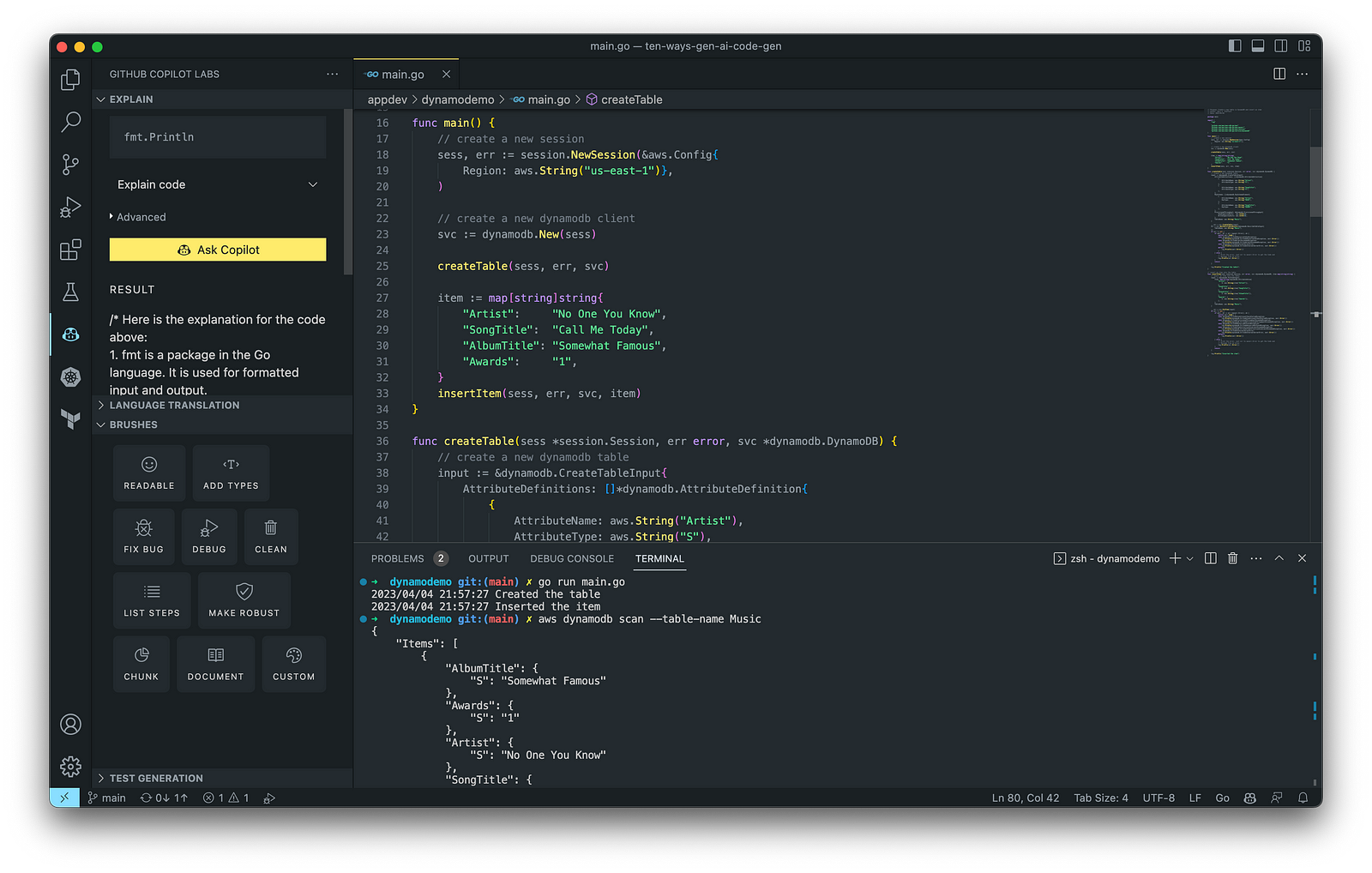
1. Application Development
According to GitHub, trained on billions of lines of code, GitHub Copilot turns natural language prompts into coding suggestions across dozens of languages. These features make Copilot ideal for developing applications, writing unit tests, and authoring documentation. You can use GitHub Copilot to assist with writing software applications in nearly any popular language, including Go.
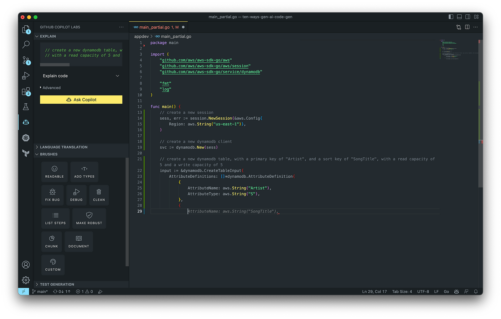
The final application, which uses the AWS SDK for Go to create an Amazon DynamoDB table, shown below, was formatted using the Go extension by Google and optimized using the ‘Readable,’ ‘Make Robust,’ and ‘Fix Bug’ GitHub Code Brushes.
Generating Unit Tests
Using JavaScript and TypeScript, you can take advantage of TestPilot to generate unit tests based on your existing code and documentation. TestPilot, part of GitHub Copilot Labs, uses GitHub Copilot’s AI technology.

2. Infrastructure as Code (IaC)
Widespread Infrastructure as Code (IaC) tools include Pulumi, AWS CloudFormation, Azure ARM Templates, Google Deployment Manager, AWS Cloud Development Kit (AWS CDK), Microsoft Bicep, and Ansible. Many IaC tools, except AWS CDK, use JSON- or YAML-based domain-specific languages (DSLs).
AWS CloudFormation
AWS CloudFormation is an Infrastructure as Code (IaC) service that allows you to easily model, provision, and manage AWS and third-party resources. The CloudFormation template is a JSON or YAML formatted text file. You can use GitHub Copilot to assist with writing IaC, including AWS CloudFormation in either JSON or YAML.

You can use the YAML Language Support by Red Hat extension to write YAML in VS Code.

VS Code has native JSON support with JSON Schema Store, which includes AWS CloudFormation. VS Code uses the CloudFormation schema for IntelliSense and flag schema errors in templates.

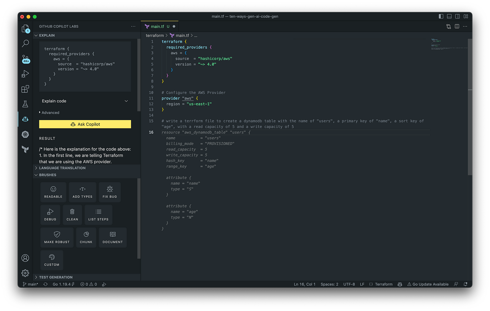
HashiCorp Terraform
In addition to AWS CloudFormation, HashiCorp Terraform is an extremely popular IaC tool. According to HashiCorp, Terraform lets you define resources and infrastructure in human-readable, declarative configuration files and manages your infrastructure’s lifecycle. Using Terraform has several advantages over manually managing your infrastructure.
Terraform plugins called providers let Terraform interact with cloud platforms and other services via their application programming interfaces (APIs). You can use the AWS Provider to interact with the many resources supported by AWS.
3. AWS Lambda
Lambda, according to AWS, is a serverless, event-driven compute service that lets you run code for virtually any application or backend service without provisioning or managing servers. You can trigger Lambda from over 200 AWS services and software as a service (SaaS) applications and only pay for what you use. AWS Lambda natively supports Java, Go, PowerShell, Node.js, C#, Python, and Ruby. AWS Lambda also provides a Runtime API allowing you to use additional programming languages to author your functions.
You can use GitHub Copilot to assist with writing AWS Lambda functions in any of the natively supported languages. You can further optimize the resulting Lambda code with GitHub’s Code Brushes.

The final Python-based AWS Lambda, below, was formatted using the Black Formatter and Flake8 extensions and optimized using the ‘Readable,’ ‘Debug,’ ‘Make Robust,’ and ‘Fix Bug’ GitHub Code Brushes.

You can easily convert the Python-based AWS Lambda to Java using GitHub Copilot Lab’s ability to translate code between languages. Install the GitHub Copilot Labs extension for VS Code to try out language translation.

4. IAM Policies
AWS Identity and Access Management (AWS IAM) is a web service that helps you securely control access to AWS resources. According to AWS, you manage access in AWS by creating policies and attaching them to IAM identities (users, groups of users, or roles) or AWS resources. A policy is an object in AWS that defines its permissions when associated with an identity or resource. IAM policies are stored on AWS as JSON documents. You can use GitHub Copilot to assist in writing IAM Policies.
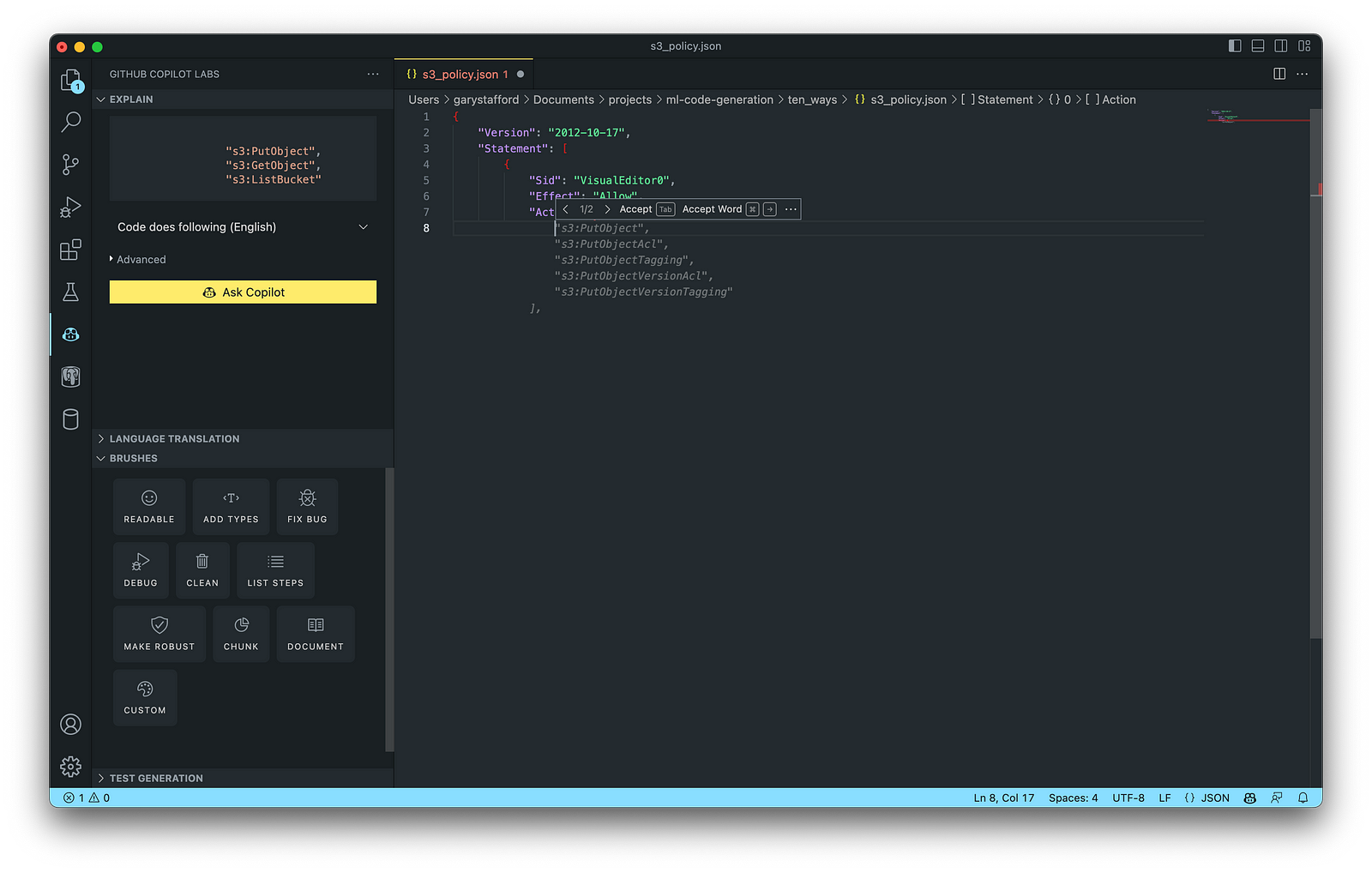
The final AWS IAM Policy, below, was formatted using VS Code’s built-in JSON support.

5. Structured Query Language (SQL)
SQL has many use cases on AWS, including Amazon Relational Database Service (RDS) for MySQL, PostgreSQL, MariaDB, Oracle, and SQL Server databases. SQL is also used with Amazon Aurora, Amazon Redshift, Amazon Athena, Apache Presto, Trino (PrestoSQL), and Apache Hive on Amazon EMR.
You can use IDEs like VS Code with its SQL dialect-specific language support and formatted extensions. You can further optimize the resulting SQL statements with GitHub’s Code Brushes.

The final PostgreSQL script, below, was formatted using the Sql Formatter extension and optimized using the ‘Readable’ and ‘Fix Bug’ GitHub Code Brushes.

6. Big Data
Big Data, according to AWS, can be described in terms of data management challenges that — due to increasing volume, velocity, and variety of data — cannot be solved with traditional databases. AWS offers managed versions of Apache Spark, Apache Flink, Apache Zepplin, and Jupyter Notebooks on Amazon EMR, AWS Glue, and Amazon Kinesis Data Analytics (KDA).
Apache Spark
According to their website, Apache Spark is a multi-language engine for executing data engineering, data science, and machine learning on single-node machines or clusters. Spark jobs can be written in various languages, including Python (PySpark), SQL, Scala, Java, and R. Apache Spark is available on a growing number of AWS services, including Amazon EMR and AWS Glue.

The final Python-based Apache Spark job, below, was formatted using the Black Formatter extension and optimized using the ‘Readable,’ ‘Document,’ ‘Make Robust,’ and ‘Fix Bug’ GitHub Code Brushes.

7. Configuration and Properties Files
According to TechTarget, a configuration file (aka config) defines the parameters, options, settings, and preferences applied to operating systems, infrastructure devices, and applications. There are many examples of configuration and properties files on AWS, including Amazon MSK Connect (Kafka Connect Source/Sink Connectors), Amazon OpenSearch (Filebeat, Logstash), and Amazon EMR (Apache Log4j, Hive, and Spark).
Kafka Connect
Kafka Connect is a tool for scalably and reliably streaming data between Apache Kafka and other systems. It makes it simple to quickly define connectors that move large collections of data into and out of Kafka. AWS offers a fully-managed version of Kafka Connect: Amazon MSK Connect. You can use GitHub Copilot to write Kafka Connect Source and Sink Connectors with Kafka Connect and Amazon MSK Connect.

The final Kafka Connect Source Connector, below, was formatted using VS Code’s built-in JSON support. It incorporates the Debezium connector for MySQL, Avro file format, schema registry, and message transformation. Debezium is a popular open source distributed platform for performing change data capture (CDC) with Kafka Connect.

8. Apache Airflow DAGs
Apache Airflow is an open-source platform for developing, scheduling, and monitoring batch-oriented workflows. Airflow’s extensible Python framework enables you to build workflows connecting with virtually any technology. DAG (Directed Acyclic Graph) is the core concept of Airflow, collecting Tasks together, organized with dependencies and relationships to say how they should run.
Amazon Managed Workflows for Apache Airflow (Amazon MWAA) is a managed orchestration service for Apache Airflow. You can use GitHub Copilot to assist in writing DAGs for Apache Airflow, to be used with Amazon MWAA.

The final Python-based Apache Spark job, below, was formatted using the Black Formatter extension. Unfortunately, based on my testing, code optimization with GitHub’s Code Brushes is impossible with Airflow DAGs.

9. Containerization
According to Check Point Software, Containerization is a type of virtualization in which all the components of an application are bundled into a single container image and can be run in isolated user space on the same shared operating system. Containers are lightweight, portable, and highly conducive to automation. AWS describes containerization as a software deployment process that bundles an application’s code with all the files and libraries it needs to run on any infrastructure.
AWS has several container services, including Amazon Elastic Container Service (Amazon ECS), Amazon Elastic Kubernetes Service (Amazon EKS), Amazon Elastic Container Registry (Amazon ECR), and AWS Fargate. Several code-based resources can benefit from a Generative AI coding tool like GitHub Copilot, including Dockerfiles, Kubernetes resources, Helm Charts, Weaveworks Flux, and ArgoCD configuration.
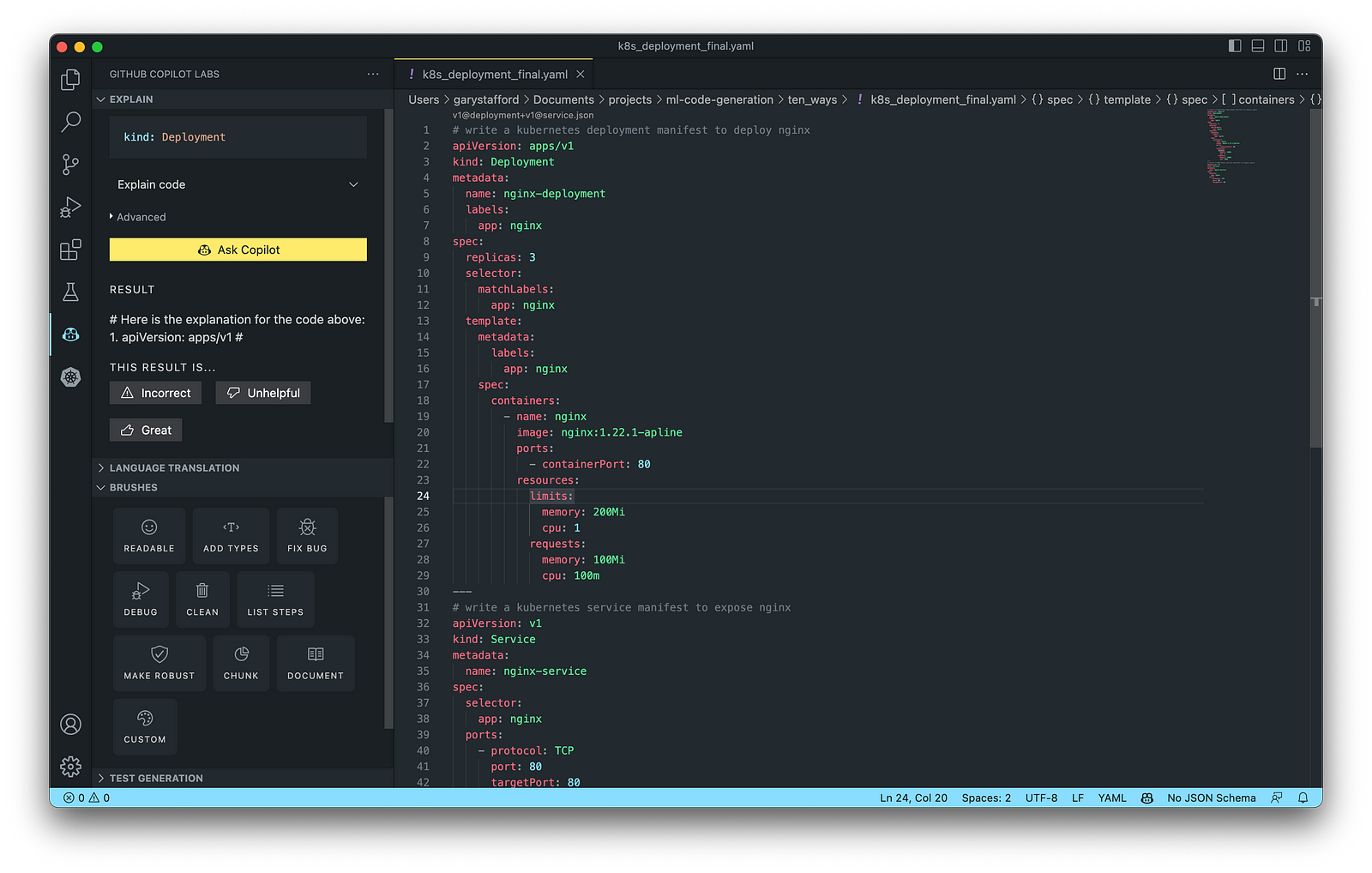
Kubernetes
Kubernetes objects are represented in the Kubernetes API and expressed in YAML format. Below is a Kubernetes Deployment resource file, which creates a ReplicaSet to bring up multiple replicas of nginx Pods.

The final Kubernetes resource file below contains Deployment and Service resources. In addition to GitHub Copilot, you can use Microsoft’s Kubernetes extension for VS Code to use IntelliSense and flag schema errors in the file.
10. Utility Scripts
According to Bing AI — Search, utility scripts are small, simple snippets of code written as independent code files designed to perform a particular task. Utility scripts are commonly written in Bash, Shell, Python, Ruby, PowerShell, and PHP.
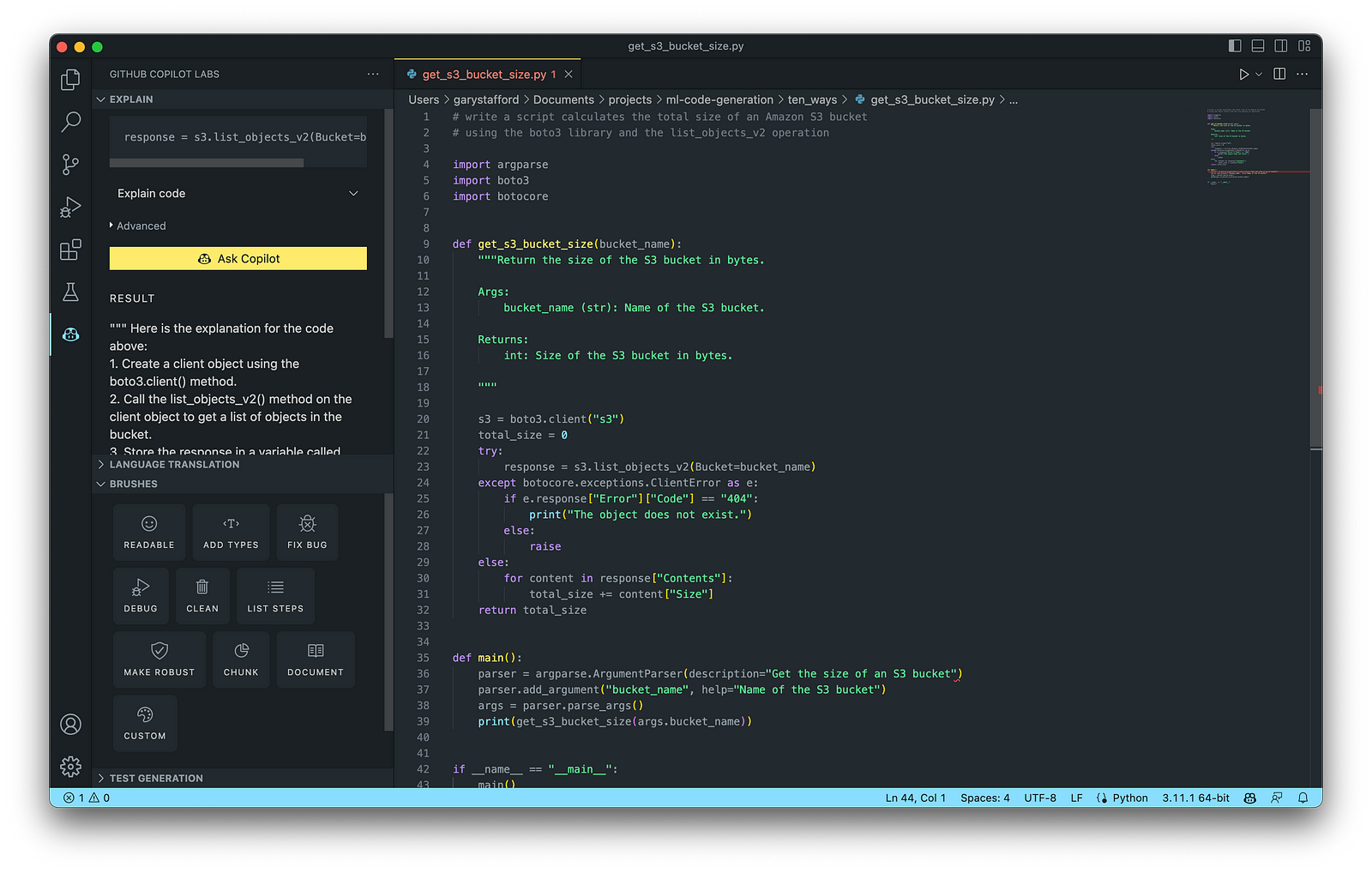
AWS utility scripts leverage the AWS Command Line Interface (AWS CLI) for Bash and Shell and AWS SDK for other programming languages. SDKs take the complexity out of coding by providing language-specific APIs for AWS services. For example, Boto3, AWS’s Python SDK, easily integrates your Python application, library, or script with AWS services, including Amazon S3, Amazon EC2, Amazon DynamoDB, and more.

An example of a Python script to calculate the total size of an Amazon S3 bucket, below, was inspired by 100daysofdevops/N-days-of-automation, a fantastic set of open source AWS-oriented automation scripts.
Conclusion
In this post, you learned ten ways to leverage Generative AI coding tools like GitHub Copilot for development on AWS. You saw how combining the latest generation of Generative AI coding tools, a mature and extensible IDE, and your coding experience will accelerate development, increase productivity, and reduce cost.
🔔 To keep up with future content, follow Gary Stafford on LinkedIn.
This blog represents my viewpoints and not those of my employer, Amazon Web Services (AWS). All product names, logos, and brands are the property of their respective owners.
End-to-End Data Discovery, Observability, and Governance on AWS with LinkedIn’s Open-source DataHub
Posted by Gary A. Stafford in Analytics, AWS, Azure, Bash Scripting, Build Automation, Cloud, DevOps, GCP, Kubernetes, Python, Software Development, SQL, Technology Consulting on March 26, 2022
Use DataHub’s data catalog capabilities to collect, organize, enrich, and search for metadata across multiple platforms
Introduction
According to Shirshanka Das, Founder of LinkedIn DataHub, Apache Gobblin, and Acryl Data, one of the simplest definitions for a data catalog can be found on the Oracle website: “Simply put, a data catalog is an organized inventory of data assets in the organization. It uses metadata to help organizations manage their data. It also helps data professionals collect, organize, access, and enrich metadata to support data discovery and governance.”
Another succinct description of a data catalog’s purpose comes from Alation: “a collection of metadata, combined with data management and search tools, that helps analysts and other data users to find the data that they need, serves as an inventory of available data, and provides information to evaluate the fitness of data for intended uses.”
Working with many organizations in the area of Analytics, one of the more common requests I receive regards choosing and implementing a data catalog. Organizations have datasources hosted in corporate data centers, on AWS, by SaaS providers, and with other Cloud Service Providers. Several of these organizations have recently gravitated to DataHub, the open-source metadata platform for the modern data stack, originally developed by LinkedIn.

In this post, we will explore the capabilities of DataHub to build a centralized data catalog on AWS for datasources hosted in multiple AWS accounts, SaaS providers, cloud service providers, and corporate data centers. I will demonstrate how to build a DataHub data catalog using out-of-the-box data source plugins for automated metadata ingestion.
Data Catalog Competitors
Data catalogs are not new; technologies such as data dictionaries have been around as far back as the 1980’s. Gartner publishes their Metadata Management (EMM) Solutions Reviews and Ratings and Metadata Management Magic Quadrant. These reports contain a comprehensive list of traditional commercial enterprise players, modern cloud-native SaaS vendors, and Cloud Service Provider (CSP) offerings. DBMS Tools also hosts a comprehensive list of 30 data catalogs. A sampling of current data catalogs includes:
Open Source Software
Commercial
- Acryl Data (based on LinkedIn’s DataHub)
- Atlan
- Stemma (based on Lyft’s Amundsen)
- Talend
- Alation
- Collibra
- data.world
Cloud Service Providers
Data Catalog Features
DataHub describes itself as “a modern data catalog built to enable end-to-end data discovery, data observability, and data governance.” Sorting through vendor’s marketing jargon and hype, standard features of leading data catalogs include:
- Metadata ingestion
- Data discovery
- Data governance
- Data observability
- Data lineage
- Data dictionary
- Data classification
- Usage/popularity statistics
- Sensitive data handling
- Data fitness (aka data quality or data profiling)
- Manage both technical and business metadata
- Business glossary
- Tagging
- Natively supported datasource integrations
- Advanced metadata search
- Fine-grain authentication and authorization
- UI- and API-based interaction
Datasources
When considering a data catalog solution, in my experience, the most common datasources that customers want to discover, inventory, and search include:
- Relational databases and other OLTP datasources such as PostgreSQL, MySQL, Microsoft SQL Server, and Oracle
- Cloud Data Warehouses and other OLAP datasources such as Amazon Redshift, Snowflake, and Google BigQuery
- NoSQL datasources such as MongoDB, MongoDB Atlas, and Azure Cosmos DB
- Persistent event-streaming platforms such as Apache Kafka (Amazon MSK and Confluent)
- Distributed storage datasets (e.g., Data Lakes) such as Amazon S3, Apache Hive, and AWS Glue Data Catalogs
- Business Intelligence (BI), dashboards, and data visualization sources such as Looker, Tableau, and Microsoft Power BI
- ETL sources, such as Apache Spark, Apache Airflow, Apache NiFi, and dbt
DataHub on AWS
DataHub’s convenient AWS setup guide covers options to deploy DataHub to AWS. For this post, I have hosted DataHub on Kubernetes, using Amazon Elastic Kubernetes Service (Amazon EKS). Alternately, you could choose Google Kubernetes Engine (GKE) on Google Cloud or Azure Kubernetes Service (AKS) on Microsoft Azure.
Conveniently, DataHub offers a Helm chart, making deployment to Kubernetes straightforward. Furthermore, Helm charts are easily integrated with popular CI/CD tools. For this post, I’ve used ArgoCD, the declarative GitOps continuous delivery tool for Kubernetes, to deploy the DataHub Helm charts to Amazon EKS.

According to the documentation, DataHub consists of four main components: GMS, MAE Consumer (optional), MCE Consumer (optional), and Frontend. Kubernetes deployment for each of the components is defined as sub-charts under the main DataHub Helm chart.
External Storage Layer Dependencies
Four external storage layer dependencies power the main DataHub components: Kafka, Local DB (MySQL, Postgres, or MariaDB), Search Index (Elasticsearch), and Graph Index (Neo4j or Elasticsearch). DataHub has provided a separate DataHub Prerequisites Helm chart for the dependencies. The dependencies must be deployed before deploying DataHub.
Alternately, you can substitute AWS managed services for the external storage layer dependencies, which is also detailed in the Deploying to AWS documentation. AWS managed service dependency substitutions include Amazon RDS for MySQL, Amazon OpenSearch (fka Amazon Elasticsearch), and Amazon Managed Streaming for Apache Kafka (Amazon MSK). According to DataHub, support for using AWS Neptune as the Graph Index is coming soon.
DataHub CLI and Plug-ins
DataHub comes with the datahub CLI, allowing you to perform many common operations on the command line. You can install and use the DataHub CLI within your development environment or integrate it with your CI/CD tooling.

DataHub uses a plugin architecture. Plugins allow you to install only the datasource dependencies you need. For example, if you want to ingest metadata from Amazon Athena, just install the Athena plugin: pip install 'acryl-datahub[athena]'. DataHub Source, Sink, and Transformer plugins can be displayed using the datahub check plugins CLI command.


Secure Metadata Ingestion
Often, datasources are not externally accessible for security reasons. Further, many datasources may not be accessible to individual users, especially in higher environments like UAT, Staging, and Production. They are only accessible to applications or CI/CD tooling. To overcome these limitations when extracting metadata with DataHub, I prefer to perform my DataHub-related development and testing locally but execute all DataHub ingestion securely on AWS.
In my local development environment, I use JetBrains PyCharm to author the Python and YAML-based DataHub configuration files and ingestion pipeline recipes, then commit those files to git and push them to a private GitHub repository. Finally, I use GitHub Actions to test DataHub files.
To run DataHub ingestion jobs and push the results to DataHub running in Kubernetes on Amazon EKS, I have built a custom Python-based Docker container. The container runs the DataHub CLI, required DataHub plugins, and any additional Python dependencies. The container’s pod has the appropriate AWS IAM permissions, using IAM Roles for Service Accounts (IRSA), to securely access datasources to ingest and the DataHub application.
Schedule and Monitor Pipelines
Scheduling and managing multiple metadata ingestion jobs on AWS is best handled with Apache Airflow with Amazon Managed Workflows for Apache Airflow (Amazon MWAA). Ingestion jobs run as Airflow DAG tasks, which call the EKS-based DataHub CLI container. With MWAA, datasource connections, credentials, and other sensitive configurations can be kept secure and not be exposed externally or in plain text.
When running the ingestion pipelines on AWS with DataHub, all communications between AWS-based datasources, ingestion jobs running in Airflow, and DataHub, should use secure private IP addressing and DNS resolution instead of transferring metadata over the Internet. Make sure to create all the necessary VPC peering connections, network route table configurations, and VPC endpoints to connect all relevant services.
SaaS services such as Snowflake or MongoDB Atlas, services provided by other Cloud Service Providers such as Google Cloud and Microsoft Azure, and datasources in corporate datasources require alternate networking and security strategies to access metadata securely.

Markup or Code?
According to the documentation, a DataHub recipe is a configuration file that tells ingestion scripts where to pull data from (source) and where to put it (sink). Recipes normally contain a source, sink, and transformers configuration section. Mark-up language-based job automation written in YAML, JSON, or Domain Specific Languages (DSLs) is often an alternative to writing code. DataHub recipes can be written in YAML. The example recipe shown below is used to ingest metadata from an Amazon RDS for PostgreSQL database, running on AWS.
YAML-based recipes can also use automatic environment variable expansion for convenience, automation, and security. It is considered best practice to secure sensitive configuration values, such as database credentials, in a secure location and reference them as environment variables. For example, note the server: ${DATAHUB_REST_ENDPOINT} entry in the sink section below. The DATAHUB_REST_ENDPOINT environment variable is set ahead of time and re-used for all ingestion jobs. Sensitive database connection information has also been variablized and stored separately.
Using Python
You can configure and run a pipeline entirely from within a custom Python script using DataHub’s Python API as an alternative to YAML. Below, we see two nearly identical ingestion recipes to the YAML above, written in Python. Writing ingestion pipeline logic programmatically gives you increased flexibility for automation, error checking, unit-testing, and notification. Below is a basic pipeline written in Python. The code is functional, but not very Pythonic, secure, scalable, or Production ready.
The second version of the same pipeline is more Production ready. The code is more Pythonic in nature and makes use of error checking, logging, and the AWS Systems Manager (SSM) Parameter Store. Like recipes written in YAML, environment variables can be used for convenience and security. In this example, commonly reused and sensitive connection configuration items have been extracted and placed in the SSM Parameter Store. Additional configuration is pulled from the environment, such as AWS Account ID and AWS Region. The script loads these values at runtime.
Sinking to DataHub
When syncing metadata to DataHub, you have two choices, the GMS REST API or Kafka. According to DataHub, the advantage of the REST-based interface is that any errors can immediately be reported. On the other hand, the advantage of the Kafka-based interface is that it is asynchronous and can handle higher throughput. For this post, I am DataHub’s REST API.


Column-level Metadata
In addition to column names and data types, it is possible to extract column descriptions and key types from certain datasources. Column descriptions, tags, and glossary terms can also be input through the DataHub UI. Below, we see an example of an Amazon Redshift fact table, whose table and column descriptions were ingested as part of the metadata.

Business Glossary
DataHub can assign business glossary terms to entities. The DataHub Business Glossary plugin pulls business glossary metadata from a YAML-based configuration file.
Business glossary terms can be reviewed in the Glossary Terms tab of the DataHub’s UI. Below, we see the three terms associated with the Classification glossary node: Confidential, HighlyConfidential, and Sensitive.

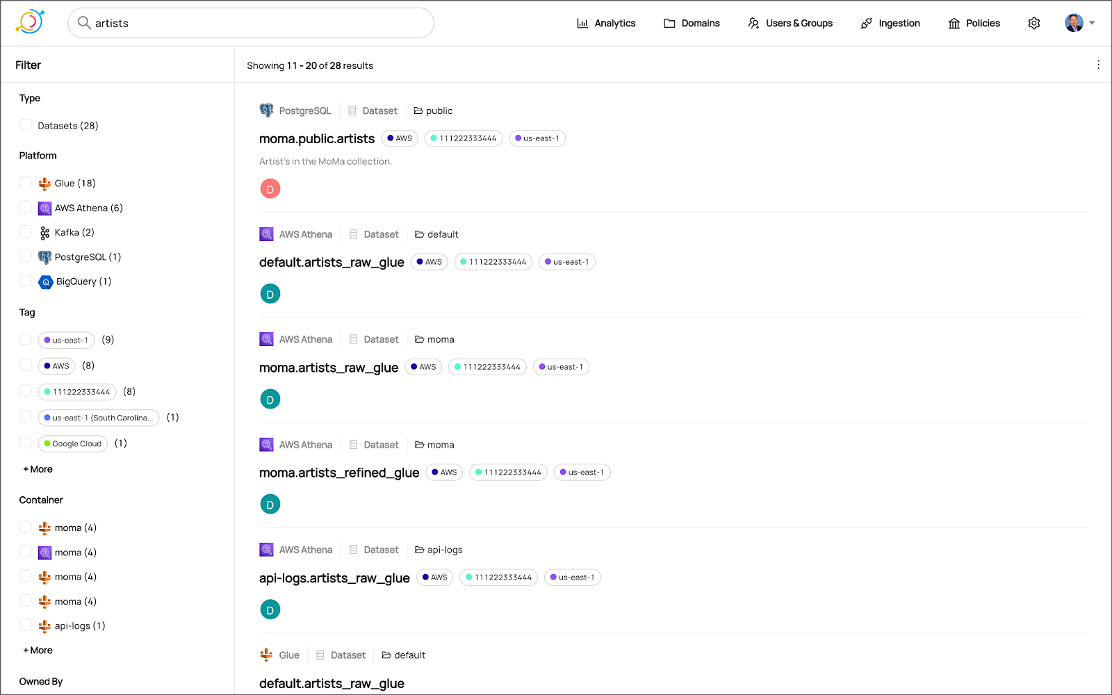
We can search for entities inventoried in DataHub using their assigned business glossary terms.

Finally, we see an example of an AWS Athena data catalog table with business glossary terms applied to columns within the table’s schema.

SQL-based Profiler
DataHub also can extract statistics about entities in DataHub using the SQL-based Profiler. According to the DataHub documentation, the Profiler can extract the following:
- Row and column counts for each table
- Column null counts and proportions
- Column distinct counts and proportions
- Column min, max, mean, median, standard deviation, quantile values
- Column histograms or frequencies of unique values
In addition, we can also track the historical stats for each profiled entity each time metadata is ingested.


Data Lineage
DataHub’s data lineage features allow us to view upstream and downstream relationships between different types of entities. DataHub can trace lineage across multiple platforms, datasets, pipelines, charts, and dashboards.
Below, we see a simple example of dataset entity-to-entity lineage in Amazon Redshift and then Apache Spark on Amazon EMR. The fact table has a downstream relationship to four database views. The views are based on SQL queries that include the upstream table as a datasource.


DataHub Analytics
DataHub provides basic metadata quality and usage analytics in the DataHub UI: user activity, counts of datasource types, business glossary terms, environments, and actions.


Conclusion
In this post, we explored the features of a data catalog and learned about some of the leading commercial and open-source data catalogs. Next, we learned how DataHub could collect, organize, enrich, and search metadata across multiple datasources. Lastly, we discovered how easy it is to catalog metadata from datasources spread across multiple CSP, SaaS providers, and corporate data centers, and centralize those results in DataHub.
In addition to the basic features reviewed in this post, DataHub offers a growing number of additional capabilities, including GraphQL and Timeline APIs, robust authentication and authorization, application monitoring observability, and Great Expectations integration. All these qualities make DataHub an excellent choice for a data catalog.
This blog represents my own viewpoints and not of my employer, Amazon Web Services (AWS). All product names, logos, and brands are the property of their respective owners.
Data Preparation on AWS: Comparing Available ELT Options to Cleanse and Normalize Data
Posted by Gary A. Stafford in Analytics, AWS, Build Automation, Cloud, Python, SQL, Technology Consulting on March 1, 2022
Comparing the features and performance of different AWS analytics services for Extract, Load, Transform (ELT)
Introduction
According to Wikipedia, “Extract, load, transform (ELT) is an alternative to extract, transform, load (ETL) used with data lake implementations. In contrast to ETL, in ELT models the data is not transformed on entry to the data lake but stored in its original raw format. This enables faster loading times. However, ELT requires sufficient processing power within the data processing engine to carry out the transformation on demand, to return the results in a timely manner.”
As capital investments and customer demand continue to drive the growth of the cloud-based analytics market, the choice of tools seems endless, and that can be a problem. Customers face a constant barrage of commercial and open-source tools for their batch, streaming, and interactive exploratory data analytics needs. The major Cloud Service Providers (CSPs) have even grown to a point where they now offer multiple services to accomplish similar analytics tasks.
This post will examine the choice of analytics services available on AWS capable of performing ELT. Specifically, this post will compare the features and performance of AWS Glue Studio, Amazon Glue DataBrew, Amazon Athena, and Amazon EMR using multiple ELT use cases and service configurations.
Analytics Use Case
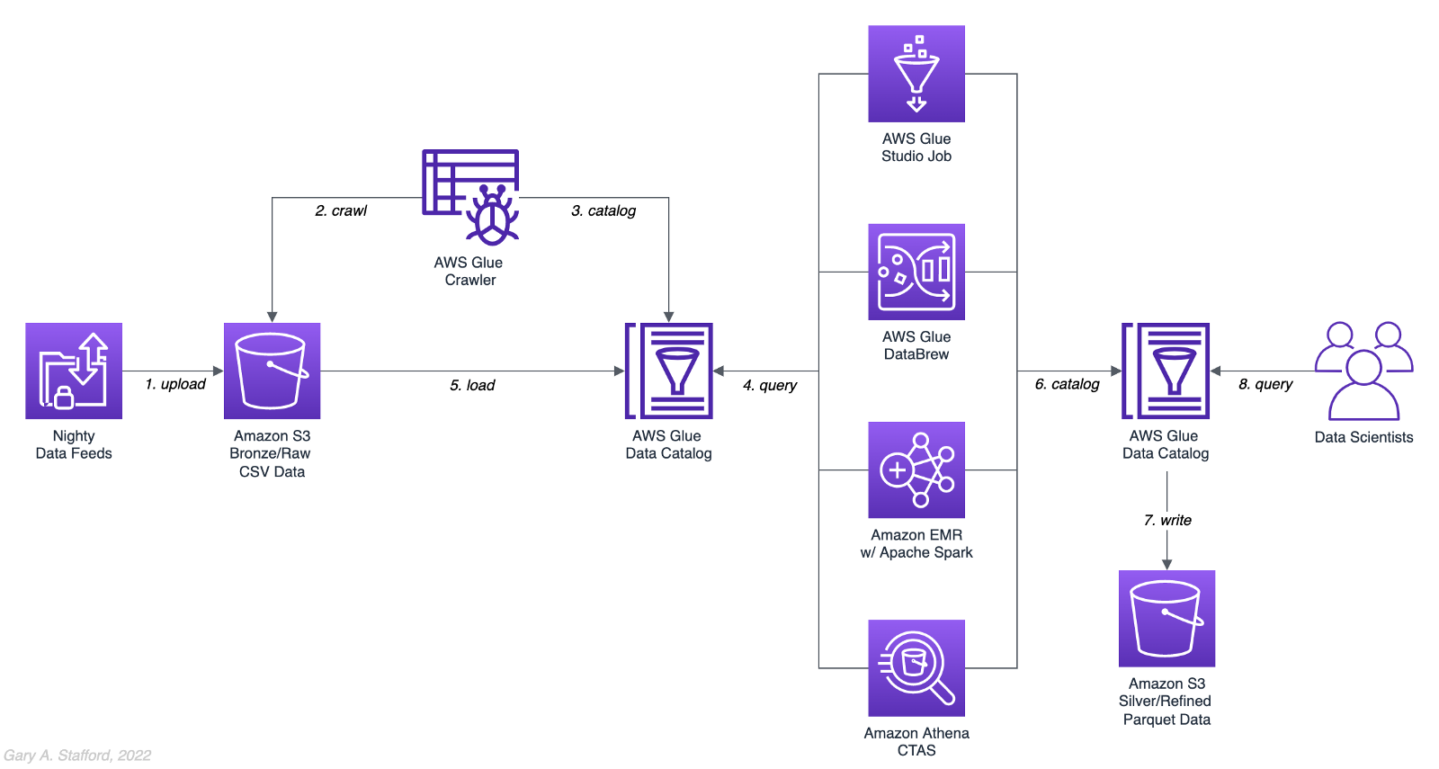
We will address a simple yet common analytics challenge for this comparison — preparing a nightly data feed for analysis the next day. Each night a batch of approximately 1.2 GB of raw CSV-format healthcare data will be exported from a Patient Administration System (PAS) and uploaded to Amazon S3. The data must be cleansed, deduplicated, refined, normalized, and made available to the Data Science team the following morning. The team of Data Scientists will perform complex data analytics on the data and build machine learning models designed for early disease detection and prevention.
Sample Dataset
The dataset used for this comparison is generated by Synthea, an open-source patient population simulation. The high-quality, synthetic, realistic patient data and associated health records cover every aspect of healthcare. The dataset contains the patient-related healthcare history for allergies, care plans, conditions, devices, encounters, imaging studies, immunizations, medications, observations, organizations, patients, payers, procedures, providers, and supplies.
The Synthea dataset was first introduced in my March 2021 post examining the handling of sensitive PII data using Amazon Macie: Data Lakes: Discovery, Security, and Privacy of Sensitive Data.
The Synthea synthetic patient data is available in different record volumes and various data formats, including HL7 FHIR, C-CDA, and CSV. We will use CSV-format data files for this post. Since this post seeks to measure the performance of different AWS ELT-capable services, we will use a larger version of the Synthea dataset containing hundreds of thousands to millions of records.
AWS Glue Data Catalog
The dataset comprises nine uncompressed CSV files uploaded to Amazon S3 and cataloged to an AWS Glue Data Catalog, a persistent metadata store, using an AWS Glue Crawler.

Test Cases
We will use three data preparation test cases based on the Synthea dataset to examine the different AWS ELT-capable services.

Test Case 1: Encounters for Symptom
An encounter is a health care contact between the patient and the provider responsible for diagnosing and treating the patient. In our first test case, we will process 1.26M encounters records for an ongoing study of patient symptoms by our Data Science team.
Data preparation includes the following steps:
- Load 1.26M encounter records using the existing AWS Glue Data Catalog table.
- Remove any duplicate records.
- Select only the records where the
descriptioncolumn contains “Encounter for symptom.” - Remove any rows with an empty
reasoncodescolumn. - Extract a new
year,month, anddaycolumn from thedatecolumn. - Remove the
datecolumn. - Write resulting dataset back to Amazon S3 as Snappy-compressed Apache Parquet files, partitioned by
year,month, andday. - Given the small resultset, bucket the data such that only one file is written per
daypartition to minimize the impact of too many small files on future query performance. - Catalog resulting dataset to a new table in the existing AWS Glue Data Catalog, including partitions.
Test Case 2: Observations
Clinical observations ensure that treatment plans are up-to-date and correctly administered and allow healthcare staff to carry out timely and regular bedside assessments. We will process 5.38M encounters records for our Data Science team in our second test case.
Data preparation includes the following steps:
- Load 5.38M observation records using the existing AWS Glue Data Catalog table.
- Remove any duplicate records.
- Extract a new
year,month, anddaycolumn from the date column. - Remove the
datecolumn. - Write resulting dataset back to Amazon S3 as Snappy-compressed Apache Parquet files, partitioned by
year,month, andday. - Given the small resultset, bucket the data such that only one file is written per
daypartition to minimize the impact of too many small files on future query performance. - Catalog resulting dataset to a new table in the existing AWS Glue Data Catalog, including partitions.
Test Case 3: Sinusitis Study
A medical condition is a broad term that includes all diseases, lesions, and disorders. In our second test case, we will join the conditions records with the patient records and filter for any condition containing the term ‘sinusitis’ in preparation for our Data Science team.
Data preparation includes the following steps:
- Load 483k condition records using the existing AWS Glue Data Catalog table.
- Inner join the condition records with the 132k patient records based on patient ID.
- Remove any duplicate records.
- Drop approximately 15 unneeded columns.
- Select only the records where the
descriptioncolumn contains the term “sinusitis.” - Remove any rows with empty
ethnicity,race,gender, ormaritalcolumns. - Create a new column,
condition_age, based on a calculation of the age in days at which the patient’s condition was diagnosed. - Write the resulting dataset back to Amazon S3 as Snappy-compressed Apache Parquet-format files. No partitions are necessary.
- Given the small resultset, bucket the data such that only one file is written to minimize the impact of too many small files on future query performance.
- Catalog resulting dataset to a new table in the existing AWS Glue Data Catalog.
AWS ELT Options
There are numerous options on AWS to handle the batch transformation use case described above; a non-exhaustive list includes:
- AWS Glue Studio (UI-driven with AWS Glue PySpark Extensions)
- Amazon Glue DataBrew
- Amazon Athena
- Amazon EMR with Apache Spark
- AWS Glue Studio (Apache Spark script)
- AWS Glue Jobs (Legacy jobs)
- Amazon EMR with Presto
- Amazon EMR with Trino
- Amazon EMR with Hive
- AWS Step Functions and AWS Lambda
- Amazon Redshift Spectrum
- Partner solutions on AWS, such as Databricks, Snowflake, Upsolver, StreamSets, Stitch, and Fivetran
- Self-managed custom solutions using a combination of OSS, such as dbt, Airbyte, Dagster, Meltano, Apache NiFi, Apache Drill, Apache Beam, Pandas, Apache Airflow, and Kubernetes
For this comparison, we will choose the first five options listed above to develop our ELT data preparation pipelines: AWS Glue Studio (UI-driven job creation with AWS Glue PySpark Extensions), Amazon Glue DataBrew, Amazon Athena, Amazon EMR with Apache Spark, and AWS Glue Studio (Apache Spark script).
AWS Glue Studio
According to the documentation, “AWS Glue Studio is a new graphical interface that makes it easy to create, run, and monitor extract, transform, and load (ETL) jobs in AWS Glue. You can visually compose data transformation workflows and seamlessly run them on AWS Glue’s Apache Spark-based serverless ETL engine. You can inspect the schema and data results in each step of the job.”
AWS Glue Studio’s visual job creation capability uses the AWS Glue PySpark Extensions, an extension of the PySpark Python dialect for scripting ETL jobs. The extensions provide easier integration with AWS Glue Data Catalog and other AWS-managed data services. As opposed to using the graphical interface for creating jobs with AWS Glue PySpark Extensions, you can also run your Spark scripts with AWS Glue Studio. In fact, we can use the exact same scripts run on Amazon EMR.
For the tests, we are using the G.2X worker type, Glue version 3.0 (Spark 3.1.1 and Python 3.7), and Python as the language choice for this comparison. We will test three worker configurations using both UI-driven job creation with AWS Glue PySpark Extensions and Apache Spark script options:
- 10 workers with a maximum of 20 DPUs
- 20 workers with a maximum of 40 DPUs
- 40 workers with a maximum of 80 DPUs


AWS Glue DataBrew
According to the documentation, “AWS Glue DataBrew is a visual data preparation tool that enables users to clean and normalize data without writing any code. Using DataBrew helps reduce the time it takes to prepare data for analytics and machine learning (ML) by up to 80 percent, compared to custom-developed data preparation. You can choose from over 250 ready-made transformations to automate data preparation tasks, such as filtering anomalies, converting data to standard formats, and correcting invalid values.”
DataBrew allows you to set the maximum number of DataBrew nodes that can be allocated when a job runs. For this comparison, we will test three different node configurations:
- 3 maximum nodes
- 10 maximum nodes
- 20 maximum nodes


Amazon Athena
According to the documentation, “Athena helps you analyze unstructured, semi-structured, and structured data stored in Amazon S3. Examples include CSV, JSON, or columnar data formats such as Apache Parquet and Apache ORC. You can use Athena to run ad-hoc queries using ANSI SQL, without the need to aggregate or load the data into Athena.”
Although Athena is classified as an ad-hoc query engine, using a CREATE TABLE AS SELECT (CTAS) query, we can create a new table in the AWS Glue Data Catalog and write to Amazon S3 from the results of a SELECT statement from another query. That other query statement performs a transformation on the data using SQL.
Amazon Athena is a fully managed AWS service and has no performance settings to adjust or monitor.


CTAS and Partitions
A notable limitation of Amazon Athena for the batch use case is the 100 partition limit with CTAS queries. Athena [only] supports writing to 100 unique partition and bucket combinations with CTAS. Partitioned by year, month, and day, the observations test case requires 2,558 partitions, and the observations test case requires 10,433 partitions. There is a recommended workaround using an INSERT INTO statement. However, the workaround requires additional SQL logic, computation, and most important cost. It is not practical, in my opinion, compared to other methods when a higher number of partitions are needed. To avoid the partition limit with CTAS, we will only partition by year and bucket by month when using Athena. Take this limitation into account when comparing the final results.
Amazon EMR with Apache Spark
According to the documentation, “Amazon EMR is a cloud big data platform for running large-scale distributed data processing jobs, interactive SQL queries, and machine learning (ML) applications using open-source analytics frameworks such as Apache Spark, Apache Hive, and Presto. You can quickly and easily create managed Spark clusters from the AWS Management Console, AWS CLI, or the Amazon EMR API.”
For this comparison, we are using two different Spark 3.1.2 EMR clusters:
- (1) r5.xlarge Master node and (2) r5.2xlarge Core nodes
- (1) r5.2xlarge Master node and (4) r5.2xlarge Core nodes
All Spark jobs are written in both Python (PySpark) and Scala. We are using the AWS Glue Data Catalog as the metastore for Spark SQL instead of Apache Hive.


Results
Data pipelines were developed and tested for each of the three test cases using the five chosen AWS ELT services and configuration variations. Each pipeline was then run 3–5 times, for a total of approximately 150 runs. The resulting AWS Glue Data Catalog table and data in Amazon S3 were deleted between each pipeline run. Each new run created a new data catalog table and wrote new results to Amazon S3. The median execution times from these tests are shown below.


Although we can make some general observations about the execution times of the chosen AWS services, the results are not meant to be a definitive guide to performance. An accurate comparison would require a deeper understanding of how each of these managed services works under the hood, in order to both optimize and balance their compute profiles correctly.
Amazon Athena
The Resultset column contains the final number of records written to Amazon S3 by Athena. The results contain the data pipeline’s median execution time and any additional data points.

AWS Glue Studio (AWS Glue PySpark Extensions)
Tests were run with three different configurations for AWS Glue Studio using the graphical interface for creating jobs with AWS Glue PySpark Extensions. Times for each configuration were nearly identical.

AWS Glue Studio (Apache PySpark script)
As opposed to using the graphical interface for creating jobs with AWS Glue PySpark Extensions, you can also run your Apache Spark scripts with AWS Glue Studio. The tests were run with the same three configurations as above. The execution times compared to the Amazon EMR tests, below, are almost identical.

Amazon EMR with Apache Spark
Tests were run with three different configurations for Amazon EMR with Apache Spark using PySpark. The first set of results is for the 2-node EMR cluster. The second set of results is for the 4-node cluster. The third set of results is for the same 4-node cluster in which the data was not bucketed into a single file within each partition. Compare the execution times and the number of objects against the previous set of results. Too many small files can negatively impact query performance.

It is commonly stated that “Scala is almost ten times faster than Python.” However, with Amazon EMR, jobs written in Python (PySpark) and Scala had similar execution times for all three test cases.

Amazon Glue DataBrew
Tests were run with three different configurations Amazon Glue DataBrew, including 3, 10, and 20 maximum nodes. Times for each configuration were nearly identical.

Observations
- All tested AWS services can read and write to an AWS Glue Data Catalog and the underlying datastore, Amazon S3. In addition, they all work with the most common analytics data file formats.
- All tested AWS services have rich APIs providing access through the AWS CLI and SDKs, which support multiple programming languages.
- Overall, AWS Glue Studio, using the AWS Glue PySpark Extensions, appears to be the most capable ELT tool of the five services tested and with the best performance.
- Both AWS Glue DataBrew and AWS Glue Studio are no-code or low-code services, democratizing access to data for non-programmers. Conversely, Amazon Athena requires knowledge of ANSI SQL, and Amazon EMR with Apache Spark requires knowledge of Scala or Python. Be cognizant of the potential trade-offs from using no-code or low-code services on observability, configuration control, and automation.
- Both AWS Glue DataBrew and AWS Glue Studio can write a custom Parquet writer type optimized for Dynamic Frames, GlueParquet. One potential advantage, a pre-computed schema is not required before writing.
- There is a slight ‘cold-start’ with Glue Studio. Studio startup times ranged from 7 seconds to 2 minutes and 4 seconds in the tests. However, the lower execution time of AWS Glue Studio compared to Amazon EMR with Spark and AWS Glue DataBrew in the tests offsets any initial cold-start time, in my opinion.
- Changing the maximum number of units from 3 to 10 to 20 for AWS Glue DataBrew made negligible differences in job execution times. Given the nearly identical execution times, it is unclear exactly how many units are being used by the job. More importantly, how many DataBrew node hours we are being billed for. These are some of the trade-offs with a fully-managed service — visibility and fine-tuning configuration.
- Similarly, with AWS Glue Studio, using either 10 workers w/ max. 20 DPUs, 20 workers w/ max. 40 DPUs, or 40 workers w/ max. 80 DPUs resulted in nearly identical executions times.
- Amazon Athena had the fastest execution times but is limited by the 100 partition limit for large CTAS resultsets. Athena is not practical, in my opinion, compared to other ELT methods, when a higher number of partitions are needed.
- It is commonly stated that “Scala is almost ten times faster than Python.” However, with Amazon EMR, jobs written in Python (PySpark) and Scala had almost identical execution times for all three test cases.
- Using Amazon EMR with EC2 instances takes about 9 minutes to provision a new cluster for this comparison fully. Given nearly identical execution times to AWS Glue Studio with Apache Spark scripts, Glue has the clear advantage of nearly instantaneous startup times.
- AWS recently announced Amazon EMR Serverless. Although this service is still in Preview, this new version of EMR could potentially reduce or eliminate the lengthy startup time for ephemeral clusters requirements.
- Although not discussed, scheduling the data pipelines to run each night was a requirement for our use case. AWS Glue Studio jobs and AWS Glue DataBrew jobs are schedulable from those services. For Amazon EMR and Amazon Athena, we could use Amazon Managed Workflows for Apache Airflow (MWAA), AWS Data Pipeline, or AWS Step Functions combined with Amazon CloudWatch Events Rules to schedule the data pipelines.
Conclusion
Customers have many options for ELT — the cleansing, deduplication, refinement, and normalization of raw data. We examined chosen services on AWS, each capable of handling the analytics use case presented. The best choice of tools depends on your specific ELT use case and performance requirements.
This blog represents my own viewpoints and not of my employer, Amazon Web Services (AWS). All product names, logos, and brands are the property of their respective owners.
DevOps for DataOps: Building a CI/CD Pipeline for Apache Airflow DAGs
Posted by Gary A. Stafford in Analytics, AWS, Big Data, Build Automation, Cloud, Continuous Delivery, DevOps, Python, Software Development, Technology Consulting on December 14, 2021
Build an effective CI/CD pipeline to test and deploy your Apache Airflow DAGs to Amazon MWAA using GitHub Actions
Introduction
In this post, we will learn how to use GitHub Actions to build an effective CI/CD workflow for our Apache Airflow DAGs. We will use the DevOps concepts of Continuous Integration and Continuous Delivery to automate the testing and deployment of Airflow DAGs to Amazon Managed Workflows for Apache Airflow (Amazon MWAA) on AWS.
Technologies
Apache Airflow
According to the documentation, Apache Airflow is an open-source platform to author, schedule, and monitor workflows programmatically. With Airflow, you author workflows as Directed Acyclic Graphs (DAGs) of tasks written in Python.
Amazon Managed Workflows for Apache Airflow
According to AWS, Amazon Managed Workflows for Apache Airflow (Amazon MWAA) is a highly available, secure, and fully-managed workflow orchestration for Apache Airflow. MWAA automatically scales its workflow execution capacity to meet your needs and is integrated with AWS security services to help provide fast and secure access to data.
GitHub Actions
According to GitHub, GitHub Actions makes it easy to automate software workflows with CI/CD. GitHub Actions allow you to build, test, and deploy code right from GitHub. GitHub Actions are workflows triggered by GitHub events like push, issue creation, or a new release. You can leverage GitHub Actions prebuilt and maintained by the community.

If you are new to GitHub Actions, I recommend my previous post, Continuous Integration and Deployment of Docker Images using GitHub Actions.
Terminology
DataOps
According to Wikipedia, DataOps is an automated, process-oriented methodology used by analytic and data teams to improve the quality and reduce the cycle time of data analytics. While DataOps began as a set of best practices, it has now matured to become a new approach to data analytics.
DataOps applies to the entire data lifecycle from data preparation to reporting and recognizes the interconnected nature of the data analytics team and IT operations. DataOps incorporates the Agile methodology to shorten the software development life cycle (SDLC) of analytics development.
DevOps
According to Wikipedia, DevOps is a set of practices that combines software development (Dev) and IT operations (Ops). It aims to shorten the systems development life cycle and provide continuous delivery with high software quality.
DevOps is a set of practices intended to reduce the time between committing a change to a system and the change being placed into normal production, while ensuring high quality. -Wikipedia
Fail Fast
According to Wikipedia, a fail-fast system is one that immediately reports any condition that is likely to indicate a failure. Using the DevOps concept of fail fast, we build steps into our workflows to uncover errors sooner in the SDLC. We shift testing as far to the left as possible (referring to the pipeline of steps moving from left to right) and test at multiple points along the way.
Source Code
All source code for this demonstration, including the GitHub Actions, Pytest unit tests, and Git Hooks, is open-sourced and located on GitHub.
Architecture
The diagram below represents the architecture for a recent blog post and video demonstration, Lakehouse Automation on AWS with Apache Airflow. The post and video show how to programmatically load and upload data from Amazon Redshift to an Amazon S3-based data lake using Apache Airflow.
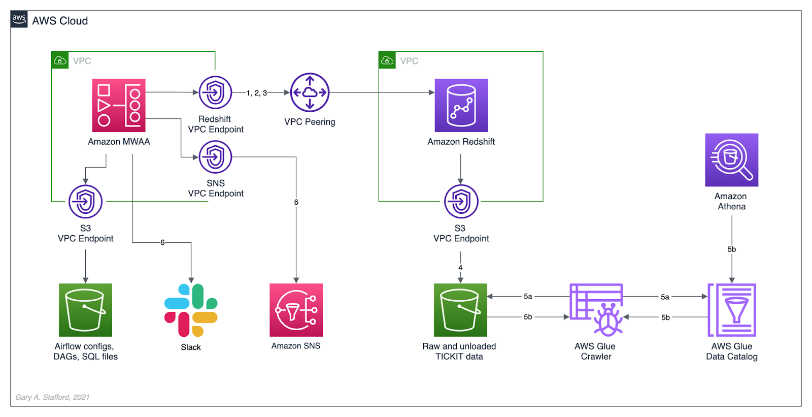
In this post, we will review how the DAGs from the previous were developed, tested, and deployed to MWAA using a variety of progressively more effective CI/CD workflows. The workflows demonstrated could also be easily applied to other Airflow resources in addition to DAGs, such as SQL scripts, configuration and data files, Python requirement files, and plugins.
Workflows
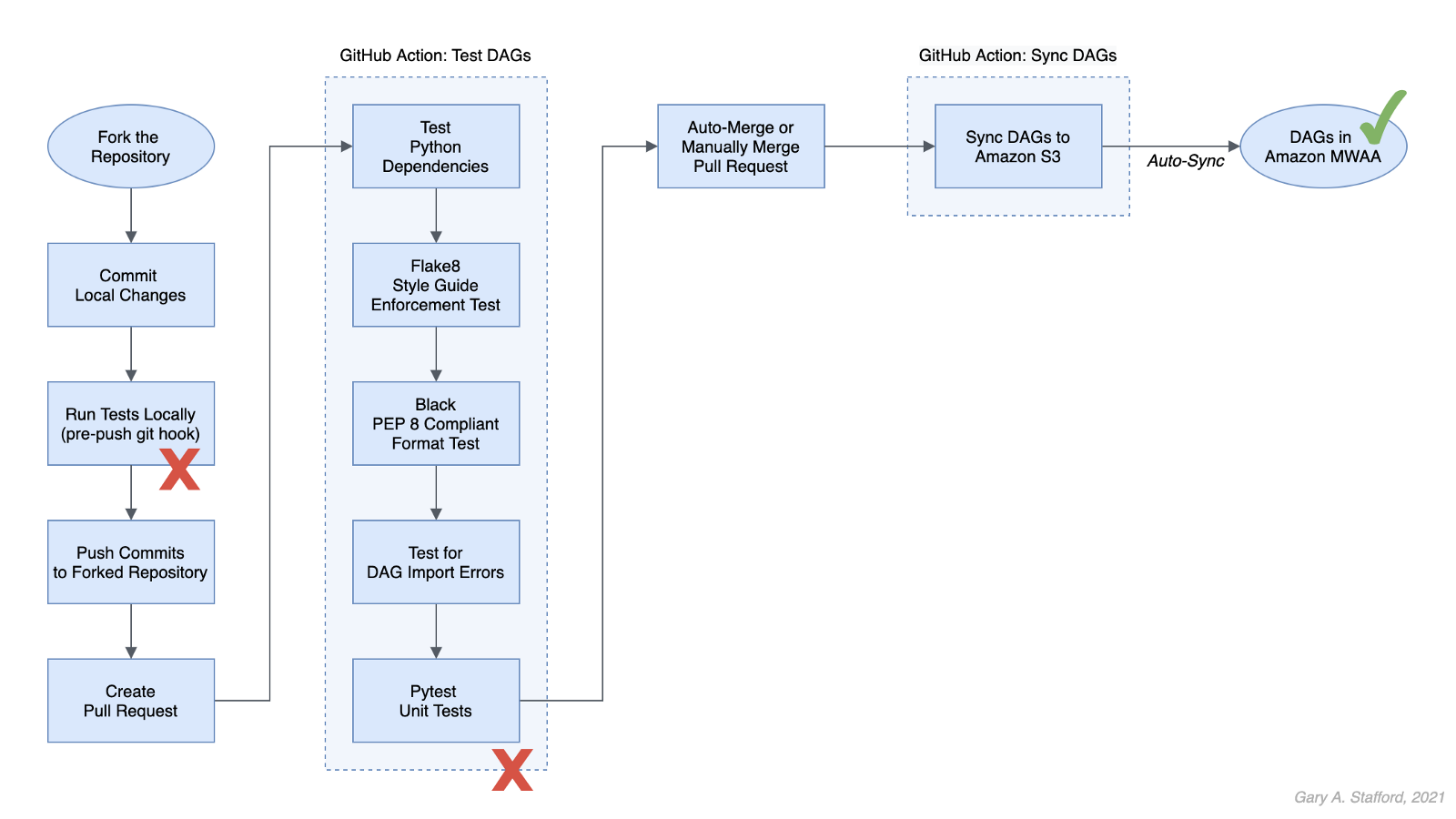
No DevOps
Below we see a minimally viable workflow for loading DAGs into Amazon MWAA, which does not use the principles of CI/CD. Changes are made in the local Airflow developer’s environment. The modified DAGs are copied directly to the Amazon S3 bucket, which are then automatically synced with Amazon MWAA, barring any errors. Those changes are also (hopefully) pushed back to the centralized version control or source code management (SCM) system, which is GitHub in this post.

There are at least two significant issues with this error-prone workflow. First, the DAGs are always out of sync between the Amazon S3 bucket and GitHub. These are two independent steps — copying or syncing the DAGs to S3 and pushing the DAGs to GitHub. A developer might continue making changes and pushing DAGs to S3 without pushing to GitHub or vice versa.
Secondly, the DevOps concept of fail-fast is missing. The first time you know your DAG contains errors is likely when it is synced to MWAA and throws an Import Error. By then, the DAG has already been copied to S3, synced to MWAA, and possibly pushed to GitHub, which other developers could then pull.

GitHub Actions
A significant step up from the previous workflow is using GitHub Actions to test and deploy your code after pushing it to GitHub. Although in this workflow, code is still ‘pushed straight to Trunk’ (the main branch in GitHub) and risks other developers in a collaborative environment pulling potentially erroneous code, you have far less chance of DAG errors making it to MWAA.

Using GitHub Actions, you also eliminate human error that could result in the changes to DAGs not being synced to Amazon S3. Lastly, using this workflow improves security by eliminating the need to provide direct access to the Airflow Amazon S3 bucket to Airflow Developers.
Types of Tests
The first GitHub Action, test_dags.yml, is triggered on a push to the dags directory in the main branch of the repository. It is also triggered whenever a pull request is made for the main branch. The first GitHub Action runs a battery of tests, including checking Python dependencies, code style, code quality, DAG import errors, and unit tests. The tests catch issues with DAGs before being synced to S3 by a second GitHub Action.
name: Test DAGs

on:
  push:
    paths:
      - 'dags/**'
  pull_request:
    branches:
      - main

jobs:
  test:
    runs-on: ubuntu-latest
    steps:
    - uses: actions/checkout@v2
    - name: Set up Python
      uses: actions/setup-python@v2
      with:
        python-version: '3.7'
    - name: Install dependencies
      run: |
        python -m pip install --upgrade pip
        pip install -r requirements/requirements.txt
        pip check
    - name: Lint with Flake8
      run: |
        pip install flake8
        flake8 --ignore E501 dags --benchmark -v
    - name: Confirm Black code compliance (psf/black)
      run: |
        pip install pytest-black
        pytest dags --black -v
    - name: Test with Pytest
      run: |
        pip install pytest
        cd tests || exit
        pytest tests.py -v

Python Dependencies
The first test installs the modules listed in the requirements.txt file used locally to develop the application. This test is designed to uncover any missing or conflicting modules.
- name: Install dependencies
  run: |
    python -m pip install --upgrade pip
    pip install -r requirements/requirements.txt
    pip check
It is essential to develop your DAGs against the same version of Python and with the same version of the Python modules used in your Airflow environment. You can use the BashOperator to run shell commands to obtain the versions of Python and module installed in your Airflow environment:
python3 --version; python3 -m pip list
A snippet of log output from DAG showing Python version and Python modules available in MWAA 2.0.2:

The latest stable release of Airflow is currently version 2.2.2, released 2021-11-15. However, as of December 2021, Amazon’s latest version of MWAA 2.x is version 2.0.2, released 2021-04-19. MWAA 2.0.2 currently runs Python3 version 3.7.10.

Flake8
Known as ‘your tool for style guide enforcement,’ Flake8 is described as the modular source code checker. It is a command-line utility for enforcing style consistency across Python projects. Flake8 is a wrapper around PyFlakes, pycodestyle, and Ned Batchelder’s McCabe script. The module, pycodestyle, is a tool to check your Python code against some of the style conventions in PEP 8.
Flake8 is highly configurable, with options to ignore specific rules if not required by your development team. For example, in this demonstration, I intentionally ignored rule E501, which states that ‘line length should be limited to 72 characters.’
- name: Lint with Flake8
  run: |
    pip install flake8
    flake8 --ignore E501 dags --benchmark -v
Black
Known as ‘the uncompromising code formatter,’ Python code formatted using Black (referred to as Blackened code) looks the same regardless of the project you’re reading. Formatting becomes transparent, allowing teams to focus on the content instead. Black makes code review faster by producing the smallest diffs possible, assuming all developers are using black to format their code.
The Airflow DAGs in this GitHub repository are automatically formatted with black using a pre-commit Git Hooks before being committed and pushed to GitHub. The test confirms black code compliance.
- name: Confirm Black code compliance (psf/black)
  run: |
    pip install pytest-black
    pytest dags --black -v
Pytest
The pytest framework describes itself as a mature, fully-featured Python testing tool that helps you write better programs. The Pytest framework makes it easy to write small tests yet scales to support complex functional testing for applications and libraries.
The GitHub Action in the GitHub project, test_dags.yml, calls the tests.py file, also contained in the project.
- name: Test with Pytest
  run: |
    pip install pytest
    cd tests || exit
    pytest tests.py -v
The tests.py file contains several pytest unit tests. The tests are based on my project requirements; your tests will vary. These tests confirm that all DAGs:
- Do not contain DAG Import Errors (test catches 75% of my errors);
- Follow specific file naming conventions;
- Include a description and an owner other than ‘airflow’;
- Contain required project tags;
- Do not send emails (my projects use SNS or Slack for notifications);
- Do not retry more than three times;
import os
import sys
import pytest
from airflow.models import DagBag
sys.path.append(os.path.join(os.path.dirname(__file__), "../dags"))
sys.path.append(os.path.join(os.path.dirname(__file__), "../dags/utilities"))
# Airflow variables called from DAGs under test are stubbed out
os.environ["AIRFLOW_VAR_DATA_LAKE_BUCKET"] = "test_bucket"
os.environ["AIRFLOW_VAR_ATHENA_QUERY_RESULTS"] = "SELECT 1;"
os.environ["AIRFLOW_VAR_SNS_TOPIC"] = "test_topic"
os.environ["AIRFLOW_VAR_REDSHIFT_UNLOAD_IAM_ROLE"] = "test_role_1"
os.environ["AIRFLOW_VAR_GLUE_CRAWLER_IAM_ROLE"] = "test_role_2"
@pytest.fixture(params=["../dags/"])
def dag_bag(request):
    return DagBag(dag_folder=request.param, include_examples=False)
def test_no_import_errors(dag_bag):
    assert not dag_bag.import_errors
def test_requires_tags(dag_bag):
    for dag_id, dag in dag_bag.dags.items():
        assert dag.tags
def test_requires_specific_tag(dag_bag):
    for dag_id, dag in dag_bag.dags.items():
        try:
            assert dag.tags.index("data lake demo") >= 0
        except ValueError:
            assert dag.tags.index("redshift demo") >= 0
def test_desc_len_greater_than_fifteen(dag_bag):
    for dag_id, dag in dag_bag.dags.items():
        assert len(dag.description) > 15
def test_owner_len_greater_than_five(dag_bag):
    for dag_id, dag in dag_bag.dags.items():
        assert len(dag.owner) > 5
def test_owner_not_airflow(dag_bag):
    for dag_id, dag in dag_bag.dags.items():
        assert str.lower(dag.owner) != "airflow"
def test_no_emails_on_retry(dag_bag):
    for dag_id, dag in dag_bag.dags.items():
        assert not dag.default_args["email_on_retry"]
def test_no_emails_on_failure(dag_bag):
    for dag_id, dag in dag_bag.dags.items():
        assert not dag.default_args["email_on_failure"]
def test_three_or_less_retries(dag_bag):
    for dag_id, dag in dag_bag.dags.items():
        assert dag.default_args["retries"] <= 3
def test_dag_id_contains_prefix(dag_bag):
    for dag_id, dag in dag_bag.dags.items():
        assert str.lower(dag_id).find("__") != -1
def test_dag_id_requires_specific_prefix(dag_bag):
    for dag_id, dag in dag_bag.dags.items():
        assert str.lower(dag_id).startswith("data_lake__") \
               or str.lower(dag_id).startswith("redshift_demo__")
If you are building custom Airflow Operators, additional unit, functional, and integration tests are recommended.
Fork and Pull
We can improve on the practice of pushing directly to Trunk by implementing one of two collaborative development models, recommended by GitHub:
- The Shared repository model: uses ‘topic’ branches, which are reviewed, approved, and merged into the main branch.
- Fork and pull model: a repo is forked, changes are made, a pull request is created, the request is reviewed, and if approved, merged into the main branch.
In the fork and pull model, we create a fork of the DAG repository where we make our changes. We then commit and push those changes back to the forked repository. When ready, we create a pull request. If the pull request is approved and passes all the tests, it is manually or automatically merged into the main branch. DAGs are then synced to S3 and, eventually, to MWAA. I usually prefer to trigger merges manually once all tests have passed.
The fork and pull model greatly reduces the chance that bad code is merged to the main branch before passing all tests.

Syncing DAGs to S3
The second GitHub Action in the GitHub project, sync_dags.yml, is triggered when the previous Action, test_dags.yml, completes successfully, or in the case of the folk and pull method, the merge to the main branch is successful.
name: Sync DAGs

on:
  workflow_run:
    workflows:
      - 'Test DAGs'
    types:
      - completed
  pull_request:
    types:
      - closed

jobs:
  deploy:
    runs-on: ubuntu-latest
    if: ${{ github.event.workflow_run.conclusion == 'success' }}
    steps:
      - uses: actions/checkout@master
      - uses: jakejarvis/s3-sync-action@master
        env:
          AWS_S3_BUCKET: ${{ secrets.AWS_S3_BUCKET }}
          AWS_ACCESS_KEY_ID: ${{ secrets.AWS_ACCESS_KEY_ID }}
          AWS_SECRET_ACCESS_KEY: ${{ secrets.AWS_SECRET_ACCESS_KEY }}
          AWS_REGION: 'us-east-1'
          SOURCE_DIR: 'dags'
          DEST_DIR: 'dags'
The GitHub Action, sync_dags.yml, requires three GitHub encrypted secrets, created in advance and associated with the GitHub repository. According to GitHub, secrets are encrypted environment variables you create in an organization, repository, or repository environment. Encrypted secrets allow you to store sensitive information, such as access tokens, in your repository. The secrets that you create are available to use in GitHub Actions workflows.

The DAGs are synced to Amazon S3 and, eventually, automatically synced to MWAA.

Local Testing and Git Hooks
To further improve your CI/CD workflows, you should consider using Git Hooks. Using Git Hooks, we can ensure code is tested locally before committing and pushing changes to GitHub. Testing locally allows us to fail-faster, catching errors during development instead of once code is pushed to GitHub.

According to the documentation, Git has a way to fire off custom scripts when certain important actions occur. There are two types of hooks: client-side and server-side. Client-side hooks are triggered by operations such as committing and merging, while server-side hooks run on network operations such as receiving pushed commits.
You can use these hooks for all sorts of reasons. I often use a client-side pre-commit hook to format DAGs using black. Using a client-side pre-push Git Hook, we will ensure that tests are run before pushing the DAGs to GitHub. According to Git, The pre-push hook runs when the git push command is executed after the remote refs have been updated but before any objects have been transferred. You can use it to validate a set of ref updates before a push occurs. A non-zero exit code will abort the push. The test could instead be run as part of the pre-commit hook if they are not too time-consuming.
To use the pre-push hook, create the following file within the local repository, .git/hooks/pre-push:
#!/bin/sh
# do nothing if there are no commits to push
if [ -z "$(git log @{u}..)" ]; then
    exit 0
fi
sh ./run_tests_locally.sh
Then, run the following chmod command to make the hook executable:
chmod 755 .git/hooks/pre-push
The the pre-push hook runs the shell script, run_tests_locally.sh. The script executes nearly identical tests, locally, as the GitHub Action, test_dags.yml, does remotely on GitHub:
#!/bin/sh
echo "Starting Flake8 test..."
flake8 --ignore E501 dags --benchmark || exit 1
echo "Starting Black test..."
python3 -m pytest --cache-clear
python3 -m pytest dags/ --black -v || exit 1
echo "Starting Pytest tests..."
cd tests || exit
python3 -m pytest tests.py -v || exit 1
echo "All tests completed successfully! 🥳"
References
Here are some additional references for testing and deploying Airflow DAGs and the use of GitHub Actions:
- Astronomer: Testing Airflow DAGs (documentation)
- Astronomer: Testing Airflow to Bullet Proof Your Code (YouTube video)
- GitHub: Building and testing Python (documentation)
- Manning: Chapter 9 of Data Pipelines with Apache Airflow
This blog represents my own viewpoints and not of my employer, Amazon Web Services (AWS). All product names, logos, and brands are the property of their respective owners.
Video Demonstration: Lakehouse Automation on AWS with Apache Airflow
Posted by Gary A. Stafford in Analytics, AWS, Build Automation, Cloud, DevOps, Python, SQL, Technology Consulting on December 2, 2021
Programmatically load and upload data from Amazon Redshift to an Amazon S3-based Data Lake using Apache Airflow
Introduction
In the following video demonstration, we will learn how to programmatically load and upload data from Amazon Redshift to an Amazon S3-based Data Lake using Apache Airflow. Since we are on AWS, we will be using the fully-managed Amazon Managed Workflows for Apache Airflow (Amazon MWAA). Using Airflow, we will COPY raw data into staging tables, then merge that staging data into a series of tables. We will then load incremental data into Redshift on a regular schedule. Next, we will join and aggregate data from several tables and UNLOAD the resulting dataset to an Amazon S3-based data lake. Lastly, we will catalog the data in S3 using AWS Glue and query with Amazon Athena.

Demonstration
Source Code
The source code for this demonstration, including the Airflow DAGs, SQL statements, and data files, is open-sourced and located on GitHub.
DAGs
The DAGs included in the GitHub project are:
- redshift_demo__01_create_tables.py
- redshift_demo__02_initial_load.py
- redshift_demo__03_incremental_load.py
- redshift_demo__04_unload_data.py
- redshift_demo__05_catalog_and_query.py
- redshift_demo__06_run_dags_01_to_05.py
- redshift_demo__06B_run_dags_01_to_05.py (alt. ver. w/external notifications module)

This blog represents my own viewpoints and not of my employer, Amazon Web Services (AWS). All product names, logos, and brands are the property of their respective owners.
Video Demonstration: Building a Data Lake with Apache Airflow
Posted by Gary A. Stafford in Analytics, AWS, Big Data, Build Automation, Cloud, Python on November 12, 2021
Build a simple Data Lake on AWS using a combination of services, including Amazon Managed Workflows for Apache Airflow (Amazon MWAA), AWS Glue, AWS Glue Studio, Amazon Athena, and Amazon S3
Introduction
In the following video demonstration, we will build a simple data lake on AWS using a combination of services, including Amazon Managed Workflows for Apache Airflow (Amazon MWAA), AWS Glue Data Catalog, AWS Glue Crawlers, AWS Glue Jobs, AWS Glue Studio, Amazon Athena, Amazon Relational Database Service (Amazon RDS), and Amazon S3.
Using a series of Airflow DAGs (Directed Acyclic Graphs), we will catalog and move data from three separate data sources into our Amazon S3-based data lake. Once in the data lake, we will perform ETL (or more accurately ELT) on the raw data — cleansing, augmenting, and preparing it for data analytics. Finally, we will perform aggregations on the refined data and write those final datasets back to our data lake. The data lake will be organized around the data lake pattern of bronze (aka raw), silver (aka refined), and gold (aka aggregated) data, popularized by Databricks.

Demonstration
Source Code
The source code for this demonstration, including the Airflow DAGs, SQL files, and data files, is open-sourced and located on GitHub.
DAGs
The DAGs shown in the video demonstration have been renamed for easier project management within the Airflow UI. The DAGs included in the GitHub project are as follows:
- data_lake__01_clean_and_prep_demo.py
- data_lake__02_run_glue_crawlers_source.py
- data_lake__03_run_glue_jobs_raw.py
- data_lake__04_run_glue_jobs_refined.py
- data_lake__05_submit_athena_queries_agg.py
- data_lake__06_run_dags_01_to_05.py
This blog represents my own viewpoints and not of my employer, Amazon Web Services (AWS). All product names, logos, and brands are the property of their respective owners.
Getting Started with Spark Structured Streaming and Kafka on AWS using Amazon MSK and Amazon EMR
Posted by Gary A. Stafford in Analytics, AWS, Big Data, Build Automation, Cloud, Software Development on September 9, 2021
Exploring Apache Spark with Apache Kafka using both batch queries and Spark Structured Streaming
Introduction
Structured Streaming is a scalable and fault-tolerant stream processing engine built on the Spark SQL engine. Using Structured Streaming, you can express your streaming computation the same way you would express a batch computation on static data. In this post, we will learn how to use Apache Spark and Spark Structured Streaming with Apache Kafka. Specifically, we will utilize Structured Streaming on Amazon EMR (fka Amazon Elastic MapReduce) with Amazon Managed Streaming for Apache Kafka (Amazon MSK). We will consume from and publish to Kafka using both batch and streaming queries. Spark jobs will be written in Python with PySpark for this post.
Apache Spark
According to the documentation, Apache Spark is a unified analytics engine for large-scale data processing. It provides high-level APIs in Java, Scala, Python (PySpark), and R, and an optimized engine that supports general execution graphs. In addition, Spark supports a rich set of higher-level tools, including Spark SQL for SQL and structured data processing, MLlib for machine learning, GraphX for graph processing, and Structured Streaming for incremental computation and stream processing.

Spark Structured Streaming
According to the documentation, Spark Structured Streaming is a scalable and fault-tolerant stream processing engine built on the Spark SQL engine. You can express your streaming computation the same way you would express a batch computation on static data. The Spark SQL engine will run it incrementally and continuously and update the final result as streaming data continues to arrive. In short, Structured Streaming provides fast, scalable, fault-tolerant, end-to-end, exactly-once stream processing without the user having to reason about streaming.
Amazon EMR
According to the documentation, Amazon EMR (fka Amazon Elastic MapReduce) is a cloud-based big data platform for processing vast amounts of data using open source tools such as Apache Spark, Hadoop, Hive, HBase, Flink, and Hudi, and Presto. Amazon EMR is a fully managed AWS service that makes it easy to set up, operate, and scale your big data environments by automating time-consuming tasks like provisioning capacity and tuning clusters.
A deployment option for Amazon EMR since December 2020, Amazon EMR on EKS, allows you to run Amazon EMR on Amazon Elastic Kubernetes Service (Amazon EKS). With the EKS deployment option, you can focus on running analytics workloads while Amazon EMR on EKS builds, configures, and manages containers for open-source applications.
If you are new to Amazon EMR for Spark, specifically PySpark, I recommend an earlier two-part series of posts, Running PySpark Applications on Amazon EMR: Methods for Interacting with PySpark on Amazon Elastic MapReduce.
Apache Kafka
According to the documentation, Apache Kafka is an open-source distributed event streaming platform used by thousands of companies for high-performance data pipelines, streaming analytics, data integration, and mission-critical applications.
Amazon MSK
Apache Kafka clusters are challenging to set up, scale, and manage in production. According to the documentation, Amazon MSK is a fully managed AWS service that makes it easy for you to build and run applications that use Apache Kafka to process streaming data. With Amazon MSK, you can use native Apache Kafka APIs to populate data lakes, stream changes to and from databases, and power machine learning and analytics applications.
Prerequisites
This post will focus primarily on configuring and running Apache Spark jobs on Amazon EMR. To follow along, you will need the following resources deployed and configured on AWS:
- Amazon S3 bucket (holds Spark resources and output);
- Amazon MSK cluster (using IAM Access Control);
- Amazon EKS container or an EC2 instance with the Kafka APIs installed and capable of connecting to Amazon MSK;
- Connectivity between the Amazon EKS cluster or EC2 and Amazon MSK cluster;
- Ensure the Amazon MSK Configuration has
auto.create.topics.enable=true; this setting isfalseby default;
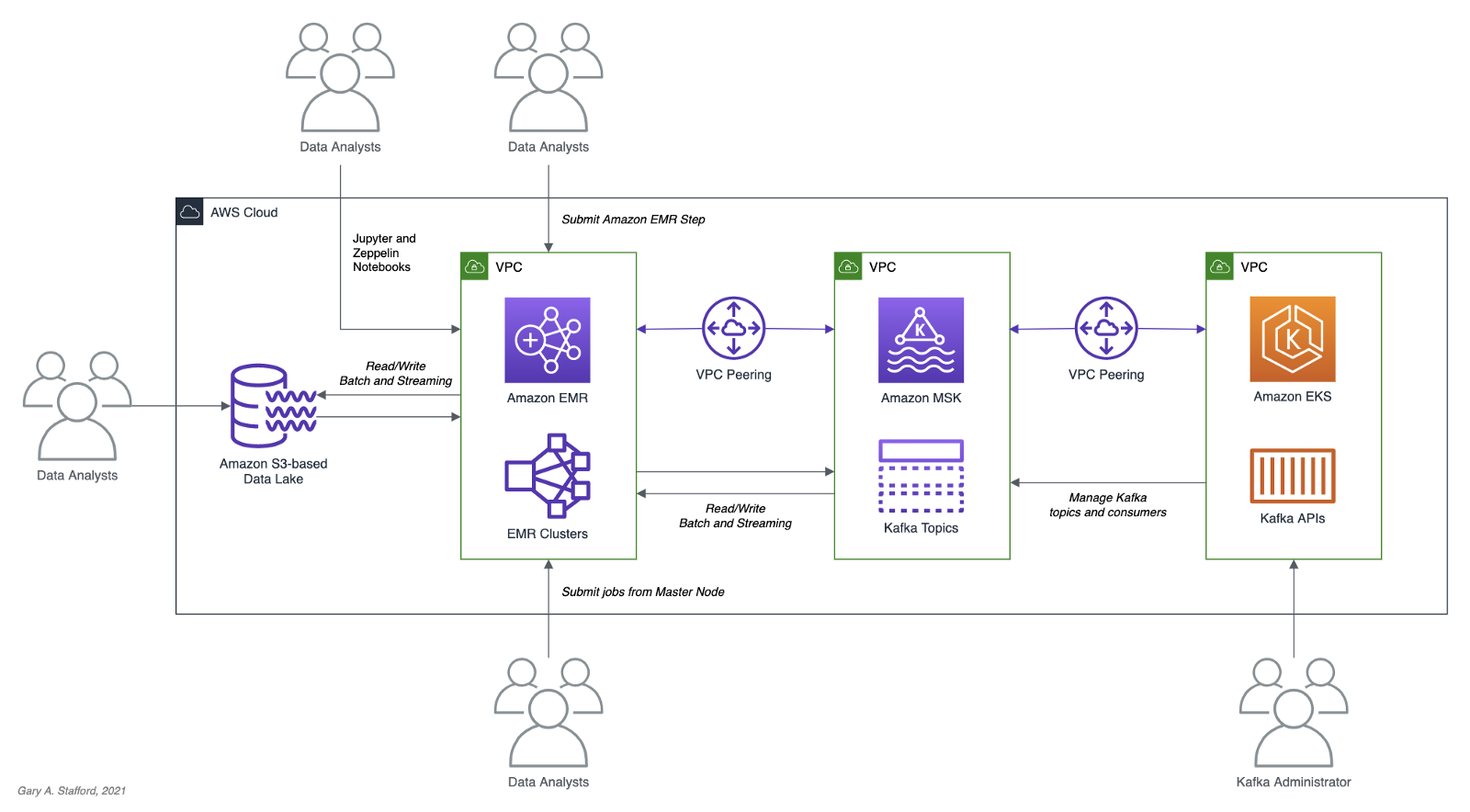
As shown in the architectural diagram above, the demonstration uses three separate VPCs within the same AWS account and AWS Region, us-east-1, for Amazon EMR, Amazon MSK, and Amazon EKS. The three VPCs are connected using VPC Peering. Ensure you expose the correct ingress ports and the corresponding CIDR ranges within your Amazon EMR, Amazon MSK, and Amazon EKS Security Groups. For additional security and cost savings, use a VPC endpoint for private communications between Amazon EMR and Amazon S3.
Source Code
All source code for this post and the two previous posts in the Amazon MSK series, including the Python/PySpark scripts demonstrated here, are open-sourced and located on GitHub.
PySpark Scripts
According to the Apache Spark documentation, PySpark is an interface for Apache Spark in Python. It allows you to write Spark applications using Python API. PySpark supports most of Spark’s features such as Spark SQL, DataFrame, Streaming, MLlib (Machine Learning), and Spark Core.
There are nine Python/PySpark scripts covered in this post:
- Initial sales data published to Kafka
01_seed_sales_kafka.py - Batch query of Kafka
02_batch_read_kafka.py - Streaming query of Kafka using grouped aggregation
03_streaming_read_kafka_console.py - Streaming query using sliding event-time window
04_streaming_read_kafka_console_window.py - Incremental sales data published to Kafka
05_incremental_sales_kafka.py - Streaming query from/to Kafka using grouped aggregation
06_streaming_read_kafka_kafka.py - Batch query of streaming query results in Kafka
07_batch_read_kafka.py - Streaming query using static join and sliding window
08_streaming_read_kafka_join_window.py - Streaming query using static join and grouped aggregation
09_streaming_read_kafka_join.py
Amazon MSK Authentication and Authorization
Amazon MSK provides multiple authentication and authorization methods to interact with the Apache Kafka APIs. For this post, the PySpark scripts use Kafka connection properties specific to IAM Access Control. You can use IAM to authenticate clients and to allow or deny Apache Kafka actions. Alternatively, you can use TLS or SASL/SCRAM to authenticate clients and Apache Kafka ACLs to allow or deny actions. In a recent post, I demonstrated the use of SASL/SCRAM and Kafka ACLs with Amazon MSK:Securely Decoupling Applications on Amazon EKS using Kafka with SASL/SCRAM.
Language Choice
According to the latest Spark 3.1.2 documentation, Spark runs on Java 8/11, Scala 2.12, Python 3.6+, and R 3.5+. The Spark documentation contains code examples written in all four languages and provides sample code on GitHub for Scala, Java, Python, and R. Spark is written in Scala.

There are countless posts and industry opinions on choosing the best language for Spark. Taking no sides, I have selected the language I use most frequently for data analytics, Python using PySpark. Compared to Scala, these two languages exhibit some of the significant differences: compiled versus interpreted, statically-typed versus dynamically-typed, JVM- versus non-JVM-based, Scala’s support for concurrency and true multi-threading, and Scala’s 10x raw performance versus the perceived ease-of-use, larger community, and relative maturity of Python.
Preparation
Amazon S3
We will start by gathering and copying the necessary files to your Amazon S3 bucket. The bucket will serve as the location for the Amazon EMR bootstrap script, additional JAR files required by Spark, PySpark scripts, CSV-format data files, and eventual output from the Spark jobs.
There are a small set of additional JAR files required by the Spark jobs we will be running. Download the JARs from Maven Central and GitHub, and place them in the emr_jars project directory. The JARs will include AWS MSK IAM Auth, AWS SDK, Kafka Client, Spark SQL for Kafka, Spark Streaming, and other dependencies.
cd ./pyspark/emr_jars/
wget https://github.com/aws/aws-msk-iam-auth/releases/download/1.1.0/aws-msk-iam-auth-1.1.0-all.jar
wget https://repo1.maven.org/maven2/software/amazon/awssdk/bundle/2.17.28/bundle-2.17.28.jar
wget https://repo1.maven.org/maven2/org/apache/commons/commons-pool2/2.11.0/commons-pool2-2.11.0.jar
wget https://repo1.maven.org/maven2/org/apache/kafka/kafka-clients/2.8.0/kafka-clients-2.8.0.jar
wget https://repo1.maven.org/maven2/org/apache/spark/spark-sql-kafka-0-10_2.12/3.1.2/spark-sql-kafka-0-10_2.12-3.1.2.jar
wget https://repo1.maven.org/maven2/org/apache/spark/spark-streaming_2.12/3.1.2/spark-streaming_2.12-3.1.2.jar
wget https://repo1.maven.org/maven2/org/apache/spark/spark-tags_2.12/3.1.2/spark-tags_2.12-3.1.2.jar
wget https://repo1.maven.org/maven2/org/apache/spark/spark-token-provider-kafka-0-10_2.12/3.1.2/spark-token-provider-kafka-0-10_2.12-3.1.2.jar
Next, update the SPARK_BUCKET environment variable, then upload the JARs and all necessary project files from your copy of the GitHub project repository to your Amazon S3 bucket using the AWS s3 API.
cd ./pyspark/
export SPARK_BUCKET="<your-bucket-111222333444-us-east-1>"

aws s3 cp emr_jars/ \
  "s3://${SPARK_BUCKET}/jars/" --recursive
aws s3 cp pyspark_scripts/ \
  "s3://${SPARK_BUCKET}/spark/" --recursive
aws s3 cp emr_bootstrap/ \
  "s3://${SPARK_BUCKET}/spark/" --recursive
aws s3 cp data/ \
  "s3://${SPARK_BUCKET}/spark/" --recursive
Amazon EMR
The GitHub project repository includes a sample AWS CloudFormation template and an associated JSON-format CloudFormation parameters file. The template, stack.yml, accepts several parameters. To match your environment, you will need to update the parameter values such as SSK key, Subnet, and S3 bucket. The template will build a minimally-sized Amazon EMR cluster with one master and two core nodes in an existing VPC. The template can be easily modified to meet your requirements and budget.
aws cloudformation deploy \
    --stack-name spark-kafka-demo-dev \
    --template-file ./cloudformation/stack.yml \
    --parameter-overrides file://cloudformation/dev.json \
    --capabilities CAPABILITY_NAMED_IAM
Whether you decide to use the CloudFormation template, two essential Spark configuration items in the EMR template are the list of applications to install and the bootstrap script deployment.
Below, we see the EMR bootstrap shell script, bootstrap_actions.sh, deployed and executed on the cluster’s nodes.
The script performed several tasks, including deploying the additional JAR files we copied to Amazon S3 earlier.

AWS Systems Manager Parameter Store
The PySpark scripts in this demonstration will obtain two parameters from the AWS Systems Manager (AWS SSM) Parameter Store. They include the Amazon MSK bootstrap brokers and the Amazon S3 bucket that contains the Spark assets. Using the Parameter Store ensures that no sensitive or environment-specific configuration is hard-coded into the PySpark scripts. Modify and execute the ssm_params.sh script to create two AWS SSM Parameter Store parameters.
aws ssm put-parameter \
  --name /kafka_spark_demo/kafka_servers \
  --type String \
  --value "<b-1.your-brokers.kafka.us-east-1.amazonaws.com:9098,b-2.your-brokers.kafka.us-east-1.amazonaws.com:9098>" \
  --description "Amazon MSK Kafka broker list" \
  --overwrite

aws ssm put-parameter \
  --name /kafka_spark_demo/kafka_demo_bucket \
  --type String \
  --value "<your-bucket-111222333444-us-east-1>" \
  --description "Amazon S3 bucket" \
  --overwrite
Spark Submit Options with Amazon EMR
Amazon EMR provides multiple options to run Spark jobs. The recommended method for PySpark scripts is to use Amazon EMR Steps from the EMR console or AWS CLI to submit work to Spark installed on an EMR cluster. In the console and CLI, you do this using a Spark application step, which runs the spark-submit script as a step on your behalf. With the API, you use a Step to invoke spark-submit using command-runner.jar. Alternately, you can SSH into the EMR cluster’s master node and run spark-submit. We will employ both techniques to run the PySpark jobs.
Securely Accessing Amazon MSK from Spark
Each of the PySpark scripts demonstrated in this post uses a common pattern for accessing Amazon MSK from Amazon EMR using IAM Authentication. Whether producing or consuming messages from Kafka, the same security-related options are used to configure Spark (starting at line 10, below). The details behind each option are outlined in the Security section of the Spark Structured Streaming + Kafka Integration Guide and the Configure clients for IAM access control section of the Amazon MSK IAM access control documentation.
Data Source and Analysis Objective
For this post, we will continue to use data from PostgreSQL’s sample Pagila database. The database contains simulated movie rental data. The dataset is fairly small, making it less than ideal for ‘big data’ use cases but small enough to quickly install and minimize data storage and analytical query costs.
According to mastersindatascience.org, data analytics is “…the process of analyzing raw data to find trends and answer questions…” Using Spark, we can analyze the movie rental sales data as a batch or in near-real-time using Structured Streaming to answer different questions. For example, using batch computations on static data, we could answer the question, how do the current total all-time sales for France compare to the rest of Europe? Or, what were the total sales for India during August? Using streaming computations, we can answer questions like, what are the sales volumes for the United States during this current four-hour marketing promotional period? Or, are sales to North America beginning to slow as the Olympics are aired during prime time?
Data analytics — the process of analyzing raw data to find trends and answer questions. (mastersindatascience.org)
Batch Queries
Before exploring the more advanced topic of streaming computations with Spark Structured Streaming, let’s first use a simple batch query and a batch computation to consume messages from the Kafka topic, perform a basic aggregation, and write the output to both the console and Amazon S3.
PySpark Job 1: Initial Sales Data
Kafka supports Protocol Buffers, JSON Schema, and Avro. However, to keep things simple in this first post, we will use JSON. We will seed a new Kafka topic with an initial batch of 250 JSON-format messages. This first batch of messages represents previous online movie rental sale transaction records. We will use these sales transactions for both batch and streaming queries.
The PySpark script, 01_seed_sales_kafka.py, and the seed data file, sales_seed.csv, are both read from Amazon S3 by Spark, running on Amazon EMR. The location of the Amazon S3 bucket name and the Amazon MSK’s broker list values are pulled from AWS SSM Parameter Store using the parameters created earlier. The Kafka topic that stores the sales data, pagila.sales.spark.streaming, is created automatically by the script the first time it runs.
Update the two environment variables, then submit your first Spark job as an Amazon EMR Step using the AWS CLI and the emr API:

From the Amazon EMR console, we should observe the Spark job has been completed successfully in about 30–90 seconds.

The Kafka Consumer API allows applications to read streams of data from topics in the Kafka cluster. Using the Kafka Consumer API, from within a Kubernetes container running on Amazon EKS or an EC2 instance, we can observe that the new Kafka topic has been successfully created and that messages (initial sales data) have been published to the new Kafka topic.
export BBROKERS="b-1.your-cluster.kafka.us-east-1.amazonaws.com:9098,b-2.your-cluster.kafka.us-east-1.amazonaws.com:9098, ..."
bin/kafka-console-consumer.sh \
  --topic pagila.sales.spark.streaming \
  --from-beginning \
  --property print.key=true \
  --property print.value=true \
  --property print.offset=true \
  --property print.partition=true \
  --property print.headers=true \
  --property print.timestamp=true \
  --bootstrap-server $BBROKERS \
  --consumer.config config/client-iam.properties

PySpark Job 2: Batch Query of Amazon MSK Topic
The PySpark script, 02_batch_read_kafka.py, performs a batch query of the initial 250 messages in the Kafka topic. When run, the PySpark script parses the JSON-format messages, then aggregates the data by both total sales and order count, by country, and finally, sorts by total sales.
window = Window.partitionBy("country").orderBy("amount")
window_agg = Window.partitionBy("country")
.withColumn("row", F.row_number().over(window)) \
.withColumn("orders", F.count(F.col("amount")).over(window_agg)) \
.withColumn("sales", F.sum(F.col("amount")).over(window_agg)) \
.where(F.col("row") == 1).drop("row") \
The results are written to both the console as stdout and to Amazon S3 in CSV format.
Again, submit this job as an Amazon EMR Step using the AWS CLI and the emr API:
To view the console output, click on ‘View logs’ in the Amazon EMR console, then click on the stdout logfile, as shown below.

The stdout logfile should contain the top 25 total sales and order counts, by country, based on the initial 250 sales records.
+------------------+------+------+
|country           |sales |orders|
+------------------+------+------+
|India             |138.80|20    |
|China             |133.80|20    |
|Mexico            |106.86|14    |
|Japan             |100.86|14    |
|Brazil            |96.87 |13    |
|Russian Federation|94.87 |13    |
|United States     |92.86 |14    |
|Nigeria           |58.93 |7     |
|Philippines       |58.92 |8     |
|South Africa      |46.94 |6     |
|Argentina         |42.93 |7     |
|Germany           |39.96 |4     |
|Indonesia         |38.95 |5     |
|Italy             |35.95 |5     |
|Iran              |33.95 |5     |
|South Korea       |33.94 |6     |
|Poland            |30.97 |3     |
|Pakistan          |25.97 |3     |
|Taiwan            |25.96 |4     |
|Mozambique        |23.97 |3     |
|Ukraine           |23.96 |4     |
|Vietnam           |23.96 |4     |
|Venezuela         |22.97 |3     |
|France            |20.98 |2     |
|Peru              |19.98 |2     |
+------------------+------+------+
only showing top 25 rows
The PySpark script also wrote the same results to Amazon S3 in CSV format.

The total sales and order count for 69 countries were computed, sorted, and coalesced into a single CSV file.
Streaming Queries
To demonstrate streaming queries with Spark Structured Streaming, we will use a combination of two PySpark scripts. The first script, 03_streaming_read_kafka_console.py, will perform a streaming query and computation of messages in the Kafka topic, aggregating the total sales and number of orders. Concurrently, the second PySpark script, 04_incremental_sales_kafka.py, will read additional Pagila sales data from a CSV file located on Amazon S3 and write messages to the Kafka topic at a rate of two messages per second. The first script, 03_streaming_read_kafka_console.py, will stream aggregations in micro-batches of one-minute increments to the console. Spark Structured Streaming queries are processed using a micro-batch processing engine, which processes data streams as a series of small, batch jobs.
Note that this first script performs grouped aggregations as opposed to aggregations over a sliding event-time window. The aggregated results represent the total, all-time sales at a point in time, based on all the messages currently in the topic when the micro-batch was computed.
To follow along with this part of the demonstration, you can run the two Spark jobs as concurrent steps on the existing Amazon EMR cluster, or create a second EMR cluster, identically configured to the existing cluster, to run the second PySpark script, 04_incremental_sales_kafka.py. Using a second cluster, you can use a minimally-sized single master node cluster with no core nodes to save cost.
PySpark Job 3: Streaming Query to Console
The first PySpark scripts, 03_streaming_read_kafka_console.py, performs a streaming query of messages in the Kafka topic. The script then aggregates the data by both total sales and order count, by country, and finally, sorts by total sales.
.groupBy("country") \
.agg(F.count("amount"), F.sum("amount")) \
.orderBy(F.col("sum(amount)").desc()) \
.select("country",
        (F.format_number(F.col("sum(amount)"), 2)).alias("sales"),
        (F.col("count(amount)")).alias("orders")) \
The results are streamed to the console using the processingTime trigger parameter. A trigger defines how often a streaming query should be executed and emit new data. The processingTime parameter sets a trigger that runs a micro-batch query periodically based on the processing time (e.g. ‘5 minutes’ or ‘1 hour’). The trigger is currently set to a minimal processing time of one minute for ease of demonstration.
.trigger(processingTime="1 minute") \
.outputMode("complete") \
.format("console") \
.option("numRows", 25) \
For demonstration purposes, we will run the Spark job directly from the master node of the EMR Cluster. This method will allow us to easily view the micro-batches and associated logs events as they are output to the console. The console is normally used for testing purposes. Submitting the PySpark script from the cluster’s master node is an alternative to submitting an Amazon EMR Step. Connect to the master node of the Amazon EMR cluster using SSH, as the hadoop user:
export EMR_MASTER=<your-emr-master-dns.compute-1.amazonaws.com>
export EMR_KEY_PATH=path/to/key/<your-ssk-key.pem>
ssh -i ${EMR_KEY_PATH} hadoop@${EMR_MASTER}
Submit the PySpark script, 03_streaming_read_kafka_console.py, to Spark:
export SPARK_BUCKET="<your-bucket-111222333444-us-east-1>"
spark-submit s3a://${SPARK_BUCKET}/spark/03_streaming_read_kafka_console.py
Before running the second PySpark script, 04_incremental_sales_kafka.py, let the first script run long enough to pick up the existing sales data in the Kafka topic. Within about two minutes, you should see the first micro-batch of aggregated sales results, labeled ‘Batch: 0’ output to the console. This initial micro-batch should contain the aggregated results of the existing 250 messages from Kafka. The streaming query’s first micro-batch results should be identical to the previous batch query results.
-------------------------------------------
Batch: 0
-------------------------------------------
+------------------+------+------+
|country           |sales |orders|
+------------------+------+------+
|India             |138.80|20    |
|China             |133.80|20    |
|Mexico            |106.86|14    |
|Japan             |100.86|14    |
|Brazil            |96.87 |13    |
|Russian Federation|94.87 |13    |
|United States     |92.86 |14    |
|Nigeria           |58.93 |7     |
|Philippines       |58.92 |8     |
|South Africa      |46.94 |6     |
|Argentina         |42.93 |7     |
|Germany           |39.96 |4     |
|Indonesia         |38.95 |5     |
|Italy             |35.95 |5     |
|Iran              |33.95 |5     |
|South Korea       |33.94 |6     |
|Poland            |30.97 |3     |
|Pakistan          |25.97 |3     |
|Taiwan            |25.96 |4     |
|Mozambique        |23.97 |3     |
|Ukraine           |23.96 |4     |
|Vietnam           |23.96 |4     |
|Venezuela         |22.97 |3     |
|France            |20.98 |2     |
|Peru              |19.98 |2     |
+------------------+------+------+
only showing top 25 rows
Immediately below the batch output, there will be a log entry containing information about the batch. In the log entry snippet below, note the starting and ending offsets of the topic for the Spark job’s Kafka consumer group, 0 (null) to 250, representing the initial sales data.
PySpark Job 4: Incremental Sales Data
As described earlier, the second PySpark script, 04_incremental_sales_kafka.py, reads 1,800 additional sales records from a second CSV file located on Amazon S3, sales_incremental_large.csv. The script then publishes messages to the Kafka topic at a deliberately throttled rate of two messages per second. Concurrently, the first PySpark job, still running and performing a streaming query, will consume the new Kafka messages and stream aggregated total sales and orders in micro-batches of one-minute increments to the console over a period of about 15 minutes.
Submit the second PySpark script as a concurrent Amazon EMR Step to the first EMR cluster, or submit as a step to the second Amazon EMR cluster.
The job sends a total of 1,800 messages to Kafka at a rate of two messages per second for 15 minutes. The total runtime of the job should be approximately 19 minutes, given a few minutes for startup and shutdown. Why run for so long? We want to make sure the job’s runtime will span multiple, overlapping, sliding event-time windows.
After about two minutes, return to the terminal output of the first Spark job, 03_streaming_read_kafka_console.py, running on the master node of the first cluster. As long as new messages are consumed every minute, you should see a new micro-batch of aggregated sales results stream to the console. Below we see an example of Batch 3, which reflects additional sales compared to Batch 0, shown previously. The results reflect the current all-time sales by country in real-time as the sales are published to Kafka.
-------------------------------------------
Batch: 5
-------------------------------------------
+------------------+------+------+
|country           |sales |orders|
+------------------+------+------+
|China             |473.35|65    |
|India             |393.44|56    |
|Japan             |292.60|40    |
|Mexico            |262.64|36    |
|United States     |252.65|35    |
|Russian Federation|243.65|35    |
|Brazil            |220.69|31    |
|Philippines       |191.75|25    |
|Indonesia         |142.81|19    |
|South Africa      |110.85|15    |
|Nigeria           |108.86|14    |
|Argentina         |89.86 |14    |
|Germany           |85.89 |11    |
|Israel            |68.90 |10    |
|Ukraine           |65.92 |8     |
|Turkey            |58.91 |9     |
|Iran              |58.91 |9     |
|Saudi Arabia      |56.93 |7     |
|Poland            |50.94 |6     |
|Pakistan          |50.93 |7     |
|Italy             |48.93 |7     |
|French Polynesia  |47.94 |6     |
|Peru              |45.95 |5     |
|United Kingdom    |45.94 |6     |
|Colombia          |44.94 |6     |
+------------------+------+------+
only showing top 25 rows
If we fast forward to a later micro-batch, sometime after the second incremental sales job is completed, we should see the top 25 aggregated sales by country of 2,050 messages — 250 seed plus 1,800 incremental messages.
-------------------------------------------
Batch: 20
-------------------------------------------
+------------------+--------+------+
|country           |sales   |orders|
+------------------+--------+------+
|China             |1,379.05|195   |
|India             |1,338.10|190   |
|United States     |915.69  |131   |
|Mexico            |855.80  |120   |
|Japan             |831.88  |112   |
|Russian Federation|723.95  |105   |
|Brazil            |613.12  |88    |
|Philippines       |528.27  |73    |
|Indonesia         |381.46  |54    |
|Turkey            |350.52  |48    |
|Argentina         |298.57  |43    |
|Nigeria           |294.61  |39    |
|South Africa      |279.61  |39    |
|Taiwan            |221.67  |33    |
|Germany           |199.73  |27    |
|United Kingdom    |196.75  |25    |
|Poland            |182.77  |23    |
|Spain             |170.77  |23    |
|Ukraine           |160.79  |21    |
|Iran              |160.76  |24    |
|Italy             |156.79  |21    |
|Pakistan          |152.78  |22    |
|Saudi Arabia      |146.81  |19    |
|Venezuela         |145.79  |21    |
|Colombia          |144.78  |22    |
+------------------+--------+------+
only showing top 25 rows
Compare the informational output below for Batch 20 to Batch 0, previously. Note the starting offset of the Kafka consumer group on the topic is 1986, and the ending offset is 2050. This is because all messages have been consumed from the topic and aggregated. If additional messages were streamed to Kafka while the streaming job is still running, additional micro-batches would continue to be streamed to the console every one minute.
PySpark Job 5: Aggregations over Sliding Event-time Window
In the previous example, we analyzed total all-time sales in real-time (e.g., show me the current, total, all-time sales for France compared to the rest of Europe, at regular intervals). This approach is opposed to sales made during a sliding event-time window (e.g., are the total sales for the United States trending better during this current four-hour marketing promotional period than the previous promotional period). In many cases, real-time sales during a distinct period or event window is probably a more commonly tracked KPI than total all-time sales.
If we add a sliding event-time window to the PySpark script, we can easily observe the total sales and order counts made during the sliding event-time window in real-time.
.withWatermark("timestamp", "10 minutes") \
.groupBy("country",
         F.window("timestamp", "10 minutes", "5 minutes")) \
.agg(F.count("amount"), F.sum("amount")) \
.orderBy(F.col("window").desc(),
         F.col("sum(amount)").desc()) \
Windowed totals would not include sales (messages) present in the Kafka topic before the streaming query beginning, nor in previous sliding windows. Constructing the correct query always starts with a clear understanding of the question you are trying to answer.
Below, in the abridged console output of the micro-batch from the script, 05_streaming_read_kafka_console_window.py, we see the results of three ten-minute sliding event-time windows with a five-minute overlap. The sales and order totals represent the volume sold during that window, with this micro-batch falling within the active current window, 19:30 to 19:40 UTC.
Plotting the total sales over time using sliding event-time windows, we will observe the results do not reflect a running total. Total sales only accumulate within a sliding window.

Compare these results to the results of the previous script, whose total sales reflect a running total.

PySpark Job 6: Streaming Query from/to Amazon MSK
The PySpark script, 06_streaming_read_kafka_kafka.py, performs the same streaming query and grouped aggregation as the previous script, 03_streaming_read_kafka_console.py. However, instead of outputting results to the console, the results of this job will be written to a new Kafka topic on Amazon MSK.
.format("kafka") \
.options(**options_write) \
.option("checkpointLocation", "/checkpoint/kafka/") \
Repeat the same process used with the previous script. Re-run the seed data script, 01_seed_sales_kafka.py, but update the input topic to a new name, such as pagila.sales.spark.streaming.in. Next, run the new script, 06_streaming_read_kafka_kafka.py. Give the script time to start and consume the 250 seed messages from Kafka. Then, update the input topic name and re-run the incremental data PySpark script, 04_incremental_sales_kafka.py, concurrent to the new script on the same cluster or run on the second cluster.
When run, the script, 06_streaming_read_kafka_kafka.py, will continuously consume messages from the new pagila.sales.spark.streaming.in topic and publish grouped aggregation results to a new topic, pagila.sales.spark.streaming.out.
Use the Kafka Consumer API to view new messages as the Spark job publishes them in near real-time to Kafka.
export BBROKERS="b-1.your-cluster.kafka.us-east-1.amazonaws.com:9098,b-2.your-cluster.kafka.us-east-1.amazonaws.com:9098, ..."
bin/kafka-console-consumer.sh \
  --topic pagila.sales.spark.streaming.out \
  --from-beginning \
  --property print.key=true \
  --property print.value=true \
  --property print.offset=true \
  --property print.partition=true \
  --property print.headers=true \
  --property print.timestamp=true \
  --bootstrap-server $BBROKERS \
  --consumer.config config/client-iam.properties

PySpark Job 7: Batch Query of Streaming Results from MSK
When run, the previous script produces Kafka messages containing non-windowed sales aggregations to the Kafka topic every minute. Using the next PySpark script, 07_batch_read_kafka.py, we can consume those aggregated messages using a batch query and display the most recent sales totals to the console. Each country’s most recent all-time sales totals and order counts should be identical to the previous script’s results, representing the aggregation of all 2,050 Kafka messages — 250 seed plus 1,800 incremental messages.
To get the latest total sales by country, we will consume all the messages from the output topic, group the results by country, find the maximum (max) value from the sales column for each country, and finally, display the results sorted sales in descending order.
window = Window.partitionBy("country") \
    .orderBy(F.col("timestamp").desc())
.withColumn("row", F.row_number().over(window)) \
.where(F.col("row") == 1).drop("row") \
.select("country", "sales", "orders") \
Writing the top 25 results to the console, we should see the same results as we saw in the final micro-batch (Batch 20, shown above) of the PySpark script, 03_streaming_read_kafka_console.py.
+------------------+------+------+
|country           |sales |orders|
+------------------+------+------+
|India             |948.63|190   |
|China             |936.67|195   |
|United States     |915.69|131   |
|Mexico            |855.80|120   |
|Japan             |831.88|112   |
|Russian Federation|723.95|105   |
|Brazil            |613.12|88    |
|Philippines       |528.27|73    |
|Indonesia         |381.46|54    |
|Turkey            |350.52|48    |
|Argentina         |298.57|43    |
|Nigeria           |294.61|39    |
|South Africa      |279.61|39    |
|Taiwan            |221.67|33    |
|Germany           |199.73|27    |
|United Kingdom    |196.75|25    |
|Poland            |182.77|23    |
|Spain             |170.77|23    |
|Ukraine           |160.79|21    |
|Iran              |160.76|24    |
|Italy             |156.79|21    |
|Pakistan          |152.78|22    |
|Saudi Arabia      |146.81|19    |
|Venezuela         |145.79|21    |
|Colombia          |144.78|22    |
+------------------+------+------+
only showing top 25 rows
PySpark Job 8: Streaming Query with Static Join and Sliding Window
The PySpark script, 08_streaming_read_kafka_join_window.py, performs the same streaming query and computations over sliding event-time windows as the previous script, 05_streaming_read_kafka_console_window.py. However, instead of totaling sales and orders by country, the script totals by sales and orders sales region. A sales region is composed of multiple countries in the same geographical area. The PySpark script reads in a static list of sales regions and countries from Amazon S3, sales_regions.csv.
The script then performs a join operation between the results of the streaming query and the static list of regions, joining on country. Using the join, the streaming sales data from Kafka is enriched with the sales category. Any sales record whose country does not have an assigned sales region is categorized as ‘Unassigned.’
.join(df_regions, on=["country"], how="leftOuter") \
.na.fill("Unassigned") \
Sales and orders are then aggregated by sales region, and the top 25 are output to the console every minute.
To run the job, repeat the previous process of renaming the topic (e.g., pagila.sales.spark.streaming.region), then running the initial sales data job, this script, and finally, concurrent with this script, the incremental sales data job. Below, we see a later micro-batch output to the console from the Spark job. We see three sets of sales results, by sales region, from three different ten-minute sliding event-time windows with a five-minute overlap.
PySpark Script 9: Static Join with Grouped Aggregations
As a comparison, we can exclude the sliding event-time window operations from the previous streaming query script, 08_streaming_read_kafka_join_window.py, to obtain the current, total, all-time sales by sales region. See the script, 09_streaming_read_kafka_join.py, in the project repository for details.
-------------------------------------------
Batch: 20
-------------------------------------------
+--------------+--------+------+
|sales_region  |sales   |orders|
+--------------+--------+------+
|Asia & Pacific|5,780.88|812   |
|Europe        |3,081.74|426   |
|Latin America |2,545.34|366   |
|Africa        |1,029.59|141   |
|North America |997.57  |143   |
|Middle east   |541.23  |77    |
|Unassigned    |352.47  |53    |
|Arab States   |244.68  |32    |
+--------------+--------+------+
Conclusion
In this post, we learned how to get started with Spark Structured Streaming on Amazon EMR. First, we explored how to run jobs written in Python with PySpark on Amazon EMR as Steps and directly from the EMR cluster’s master node. Next, we discovered how to produce and consume messages with Apache Kafka on Amazon MSK, using batch and streaming queries. Finally, we learned about aggregations over a sliding event-time window compared to grouped aggregations and how Structured Streaming queries are processed using a micro-batch.
In a subsequent post, we will learn how to use Apache Avro and the Apicurio Registry with PySpark on Amazon EMR to read and write Apache Avro format messages to Amazon MSK.
This blog represents my own viewpoints and not of my employer, Amazon Web Services (AWS). All product names, logos, and brands are the property of their respective owners.
Securely Decoupling Kubernetes-based Applications on Amazon EKS using Kafka with SASL/SCRAM
Posted by Gary A. Stafford in AWS, Build Automation, Cloud, DevOps, Go, Kubernetes, Software Development on July 26, 2021
Securely decoupling Go-based microservices on Amazon EKS using Amazon MSK with IRSA, SASL/SCRAM, and data encryption
Introduction
This post will explore a simple Go-based application deployed to Kubernetes using Amazon Elastic Kubernetes Service (Amazon EKS). The microservices that comprise the application communicate asynchronously by producing and consuming events from Amazon Managed Streaming for Apache Kafka (Amazon MSK).
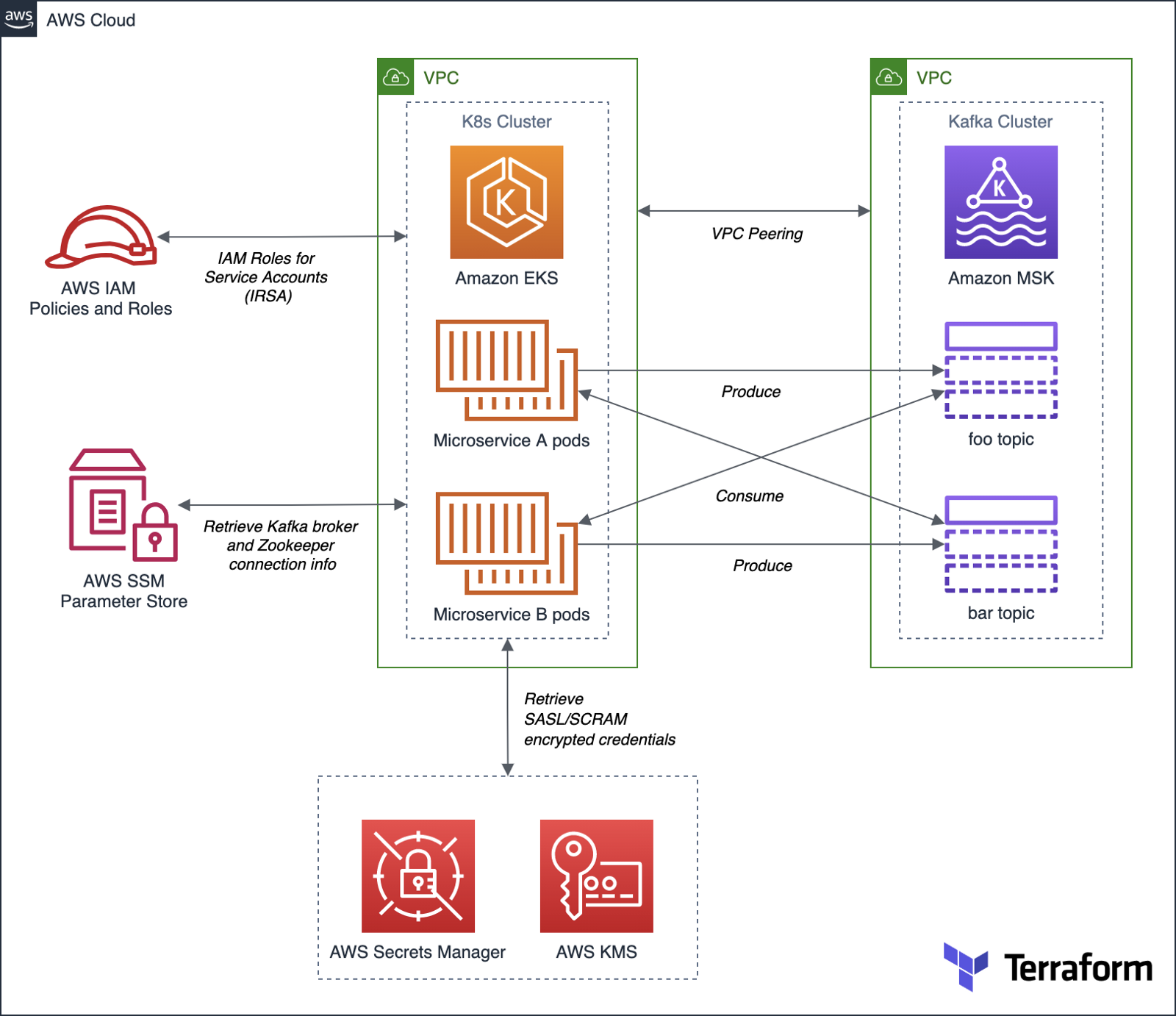
Authentication and Authorization for Apache Kafka
According to AWS, you can use IAM to authenticate clients and to allow or deny Apache Kafka actions. Alternatively, you can use TLS or SASL/SCRAM to authenticate clients, and Apache Kafka ACLs to allow or deny actions.
For this post, our Amazon MSK cluster will use SASL/SCRAM (Simple Authentication and Security Layer/Salted Challenge Response Mechanism) username and password-based authentication to increase security. Credentials used for SASL/SCRAM authentication will be securely stored in AWS Secrets Manager and encrypted using AWS Key Management Service (KMS).
Data Encryption
Data at rest in the MSK cluster will be encrypted at rest using Amazon MSK’s integration with AWS KMS to provide transparent server-side encryption. Encryption in transit of data moving between the brokers of the MSK cluster will be provided using Transport Layer Security (TLS 1.2).
Resource Management
AWS resources for Amazon MSK will be created and managed using HashiCorp Terraform, a popular open-source infrastructure-as-Code (IaC) software tool. Amazon EKS resources will be created and managed with eksctl, the official CLI for Amazon EKS sponsored by Weaveworks. Lastly, Kubernetes resources will be created and managed with Helm, the open-source Kubernetes package manager.
Demonstration Application
The Go-based microservices, which compose the demonstration application, will use Segment’s popular kafka-go client. Segment is a leading customer data platform (CDP). The microservices will access Amazon MSK using Kafka broker connection information stored in AWS Systems Manager (SSM) Parameter Store.
Source Code
All source code for this post, including the demonstration application, Terraform, and Helm resources, are open-sourced and located on GitHub.garystafford/terraform-msk-demo
Terraform project for using Amazon Managed Streaming for Apache Kafka (Amazon MSK) from Amazon Elastic Kubernetes…github.com
Prerequisites
To follow along with this post’s demonstration, you will need recent versions of terraform, eksctl, and helm installed and accessible from your terminal. Optionally, it will be helpful to have git or gh, kubectl, and the AWS CLI v2 (aws).
Demonstration
To demonstrate the EKS and MSK features described above, we will proceed as follows:
- Deploy the EKS cluster and associated resources using
eksctl; - Deploy the MSK cluster and associated resources using Terraform;
- Update the route tables for both VPCs and associated subnets to route traffic between the peered VPCs;
- Create IAM Roles for Service Accounts (IRSA) allowing access to MSK and associated services from EKS, using
eksctl; - Deploy the Kafka client container to EKS using Helm;
- Create the Kafka topics and ACLs for MSK using the Kafka client;
- Deploy the Go-based application to EKS using Helm;
- Confirm the application’s functionality;
1. Amazon EKS cluster
To begin, create a new Amazon EKS cluster using Weaveworks’ eksctl. The default cluster.yaml configuration file included in the project will create a small, development-grade EKS cluster based on Kubernetes 1.20 in us-east-1. The cluster will contain a managed node group of three t3.medium Amazon Linux 2 EC2 worker nodes. The EKS cluster will be created in a new VPC.
Set the following environment variables and then run the eksctl create cluster command to create the new EKS cluster and associated infrastructure.
export AWS_ACCOUNT=$(aws sts get-caller-identity \
    --output text --query 'Account')
export EKS_REGION="us-east-1"
export CLUSTER_NAME="eks-kafka-demo"
eksctl create cluster -f ./eksctl/cluster.yaml
In my experience, it could take up to 25-40 minutes to fully build and configure the new 3-node EKS cluster.


As part of creating the EKS cluster, eksctl will automatically deploy three AWS CloudFormation stacks containing the following resources:
- Amazon Virtual Private Cloud (VPC), subnets, route tables, NAT Gateways, security policies, and the EKS control plane;
- EKS managed node group containing Kubernetes three worker nodes;
- IAM Roles for Service Accounts (IRSA) that maps an AWS IAM Role to a Kubernetes Service Account;

Once complete, update your kubeconfig file so that you can connect to the new Amazon EKS cluster using the following AWS CLI command:
aws eks --region ${EKS_REGION} update-kubeconfig \
    --name ${CLUSTER_NAME}
Review the details of the new EKS cluster using the following eksctl command:
eksctl utils describe-stacks \
  --region ${EKS_REGION} --cluster ${CLUSTER_NAME}

Review the new EKS cluster in the Amazon Container Services console’s Amazon EKS Clusters tab.

Below, note the EKS cluster’s OpenID Connect URL. Support for IAM Roles for Service Accounts (IRSA) on the EKS cluster requires an OpenID Connect issuer URL associated with it. OIDC was configured in the cluster.yaml file; see line 8 (shown above).

The OpenID Connect identity provider, referenced in the EKS cluster’s console, created by eksctl, can be observed in the IAM Identity provider console.

2. Amazon MSK cluster
Next, deploy the Amazon MSK cluster and associated network and security resources using HashiCorp Terraform.

Before creating the AWS infrastructure with Terraform, update the location of the Terraform state. This project’s code uses Amazon S3 as a backend to store the Terraform’s state. Change the Amazon S3 bucket name to one of your existing buckets, located in the main.tf file.
terraform {
  backend "s3" {
    bucket = "terrform-us-east-1-your-unique-name"
    key    = "dev/terraform.tfstate"
    region = "us-east-1"
  }
}
Also, update the eks_vpc_id variable in the variables.tf file with the VPC ID of the EKS VPC created by eksctl in step 1.
variable "eks_vpc_id" {
  default = "vpc-your-id"
}
The quickest way to obtain the ID of the EKS VPC is by using the following AWS CLI v2 command:
aws ec2 describe-vpcs --query 'Vpcs[].VpcId' \
  --filters Name=tag:Name,Values=eksctl-eks-kafka-demo-cluster/VPC \
  --output text
Next, initialize your Terraform backend in Amazon S3 and initialize the latesthashicorp/aws provider plugin with terraform init.

Use terraform plan to generate an execution plan, showing what actions Terraform would take to apply the current configuration. Terraform will create approximately 25 AWS resources as part of the plan.

Finally, use terraform apply to create the Amazon resources. Terraform will create a small, development-grade MSK cluster based on Kafka 2.8.0 in us-east-1, containing a set of three kafka.m5.large broker nodes. Terraform will create the MSK cluster in a new VPC. The broker nodes are spread across three Availability Zones, each in a private subnet, within the new VPC.


It could take 30 minutes or more for Terraform to create the new cluster and associated infrastructure. Once complete, you can view the new MSK cluster in the Amazon MSK management console.

Below, note the new cluster’s ‘Access control method’ is SASL/SCRAM authentication. The cluster implements encryption of data in transit with TLS and encrypts data at rest using a customer-managed customer master key (CMS) in AWM KSM.

Below, note the ‘Associated secrets from AWS Secrets Manager.’ The secret, AmazonMSK_credentials, contains the SASL/SCRAM authentication credentials — username and password. These are the credentials the demonstration application, deployed to EKS, will use to securely access MSK.

The SASL/SCRAM credentials secret shown above can be observed in the AWS Secrets Manager console. Note the customer-managed customer master key (CMK), stored in AWS KMS, which is used to encrypt the secret.

3. Update route tables for VPC Peering
Terraform created a VPC Peering relationship between the new EKS VPC and the MSK VPC. However, we will need to complete the peering configuration by updating the route tables. We want to route all traffic from the EKS cluster destined for MSK, whose VPC CIDR is 10.0.0.0/22, through the VPC Peering Connection resource. There are four route tables associated with the EKS VPC. Add a new route to the route table whose name ends with ‘PublicRouteTable’, for example, rtb-0a14e6250558a4abb / eksctl-eks-kafka-demo-cluster/PublicRouteTable. Manually create the required route in this route table using the VPC console’s Route tables tab, as shown below (new route shown second in list).

Similarly, we want to route all traffic from the MSK cluster destined for EKS, whose CIDR is 192.168.0.0/16, through the same VPC Peering Connection resource. Update the single MSK VPC’s route table using the VPC console’s Route tables tab, as shown below (new route shown second in list).

4. Create IAM Roles for Service Accounts (IRSA)
With both the EKS and MSK clusters created and peered, we are ready to start deploying Kubernetes resources. Create a new namespace, kafka, which will hold the demonstration application and Kafka client pods.
export AWS_ACCOUNT=$(aws sts get-caller-identity \
    --output text --query 'Account')
export EKS_REGION="us-east-1"
export CLUSTER_NAME="eks-kafka-demo"
export NAMESPACE="kafka"
kubectl create namespace $NAMESPACE
Then using eksctl, create two IAM Roles for Service Accounts (IRSA) associated with Kubernetes Service Accounts. The Kafka client’s pod will use one of the roles, and the demonstration application’s pods will use the other role. According to the eksctl documentation, IRSA works via IAM OpenID Connect Provider (OIDC) that EKS exposes, and IAM roles must be constructed with reference to the IAM OIDC Provider described earlier in the post, and a reference to the Kubernetes Service Account it will be bound to. The two IAM policies referenced in the eksctl commands below were created earlier by Terraform.
# kafka-demo-app role
eksctl create iamserviceaccount \
  --name kafka-demo-app-sasl-scram-serviceaccount \
  --namespace $NAMESPACE \
  --region $EKS_REGION \
  --cluster $CLUSTER_NAME \
  --attach-policy-arn "arn:aws:iam::${AWS_ACCOUNT}:policy/EKSScramSecretManagerPolicy" \
  --approve \
  --override-existing-serviceaccounts
# kafka-client-msk role
eksctl create iamserviceaccount \
  --name kafka-client-msk-sasl-scram-serviceaccount \
  --namespace $NAMESPACE \
  --region $EKS_REGION \
  --cluster $CLUSTER_NAME \
  --attach-policy-arn "arn:aws:iam::${AWS_ACCOUNT}:policy/EKSKafkaClientMSKPolicy" \
  --attach-policy-arn "arn:aws:iam::${AWS_ACCOUNT}:policy/EKSScramSecretManagerPolicy" \
  --approve \
  --override-existing-serviceaccounts
# confirm successful creation of accounts
eksctl get iamserviceaccount \
  --cluster $CLUSTER_NAME \
  --namespace $NAMESPACE
kubectl get serviceaccounts -n $NAMESPACE

Recall eksctl created three CloudFormation stacks initially. With the addition of the two IAM Roles, we now have a total of five CloudFormation stacks deployed.

5. Kafka client
Next, deploy the Kafka client using the project’s Helm chart, kafka-client-msk. We will use the Kafka client to create Kafka topics and Apache Kafka ACLs. This particular Kafka client is based on a custom Docker Image that I have built myself using an Alpine Linux base image with Java OpenJDK 17, garystafford/kafka-client-msk. The image contains the latest Kafka client along with the AWS CLI v2 and a few other useful tools like jq. If you prefer an alternative, there are multiple Kafka client images available on Docker Hub.h
The Kafka client only requires a single pod. Run the following helm commands to deploy the Kafka client to EKS using the project’s Helm chart, kafka-client-msk:
cd helm/
# perform dry run to validate chart
helm install kafka-client-msk ./kafka-client-msk \
  --namespace $NAMESPACE --debug --dry-run
# apply chart resources
helm install kafka-client-msk ./kafka-client-msk \
  --namespace $NAMESPACE

Confirm the successful creation of the Kafka client pod with either of the following commands:
kubectl get pods -n kafka
kubectl describe pod -n kafka -l app=kafka-client-msk

The ability of the Kafka client to interact with Amazon MSK, AWS SSM Parameter Store, and AWS Secrets Manager is based on two IAM policies created by Terraform, EKSKafkaClientMSKPolicy and EKSScramSecretManagerPolicy. These two policies are associated with a new IAM role, which in turn, is associated with the Kubernetes Service Account, kafka-client-msk-sasl-scram-serviceaccount. This service account is associated with the Kafka client pod as part of the Kubernetes Deployment resource in the Helm chart.
6. Kafka topics and ACLs for Kafka
Use the Kafka client to create Kafka topics and Apache Kafka ACLs. First, use the kubectl exec command to execute commands from within the Kafka client container.
export KAFKA_CONTAINER=$(
  kubectl get pods -n kafka -l app=kafka-client-msk | \
    awk 'FNR == 2 {print $1}')
kubectl exec -it $KAFKA_CONTAINER -n kafka -- bash
Once successfully attached to the Kafka client container, set the following three environment variables: 1) Apache ZooKeeper connection string, 2) Kafka bootstrap brokers, and 3) ‘Distinguished-Name’ of the Bootstrap Brokers (see AWS documentation). The values for these environment variables will be retrieved from AWS Systems Manager (SSM) Parameter Store. The values were stored in the Parameter store by Terraform during the creation of the MSK cluster. Based on the policy attached to the IAM Role associated with this Pod (IRSA), the client has access to these specific parameters in the SSM Parameter store.
export ZOOKPR=$(\
  aws ssm get-parameter --name /msk/scram/zookeeper \
    --query 'Parameter.Value' --output text)
export BBROKERS=$(\
  aws ssm get-parameter --name /msk/scram/brokers \
    --query 'Parameter.Value' --output text)
export DISTINGUISHED_NAME=$(\
  echo $BBROKERS | awk -F' ' '{print $1}' | sed 's/b-1/*/g')
Use the env and grep commands to verify the environment variables have been retrieved and constructed properly. Your Zookeeper and Kafka bootstrap broker URLs will be uniquely different from the ones shown below.
env | grep 'ZOOKPR\|BBROKERS\|DISTINGUISHED_NAME'
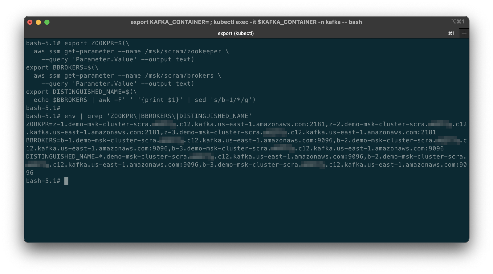
To test the connection between EKS and MSK, list the existing Kafka topics, from the Kafka client container:
bin/kafka-topics.sh --list --zookeeper $ZOOKPR
You should see three default topics, as shown below.

If you did not properly add the new VPC Peering routes to the appropriate route tables in the previous step, establishing peering of the EKS and MSK VPCs, you are likely to see a timeout error while attempting to connect. Go back and confirm that both of the route tables are correctly updated with the new routes.

Kafka Topics, Partitions, and Replicas
The demonstration application produces and consumes messages from two topics, foo-topic and bar-topic. Each topic will have three partitions, one for each of the three broker nodes, along with three replicas.

Use the following commands from the client container to create the two new Kafka topics. Once complete, confirm the creation of the topics using the list option again.
bin/kafka-topics.sh --create --topic foo-topic \
  --partitions 3 --replication-factor 3 \
  --zookeeper $ZOOKPR
bin/kafka-topics.sh --create --topic bar-topic \
  --partitions 3 --replication-factor 3 \
  --zookeeper $ZOOKPR
bin/kafka-topics.sh --list --zookeeper $ZOOKPR

Review the details of the topics using the describe option. Note the three partitions per topic and the three replicas per topic.
bin/kafka-topics.sh --describe --topic foo-topic --zookeeper $ZOOKPR
bin/kafka-topics.sh --describe --topic bar-topic --zookeeper $ZOOKPR

Kafka ACLs
According to Kafka’s documentation, Kafka ships with a pluggable Authorizer and an out-of-box authorizer implementation that uses Zookeeper to store all the Access Control Lists (ACLs). Kafka ACLs are defined in the general format of “Principal P is [Allowed/Denied] Operation O From Host H On Resource R.” You can read more about the ACL structure on KIP-11. To add, remove or list ACLs, you can use the Kafka authorizer CLI.
Authorize access by the Kafka brokers and the demonstration application to the two topics. First, allow access to the topics from the brokers using the DISTINGUISHED_NAME environment variable (see AWS documentation).
# read auth for brokers
bin/kafka-acls.sh \
  --authorizer-properties zookeeper.connect=$ZOOKPR \
  --add \
  --allow-principal "User:CN=${DISTINGUISHED_NAME}" \
  --operation Read \
  --group=consumer-group-B \
  --topic foo-topic
bin/kafka-acls.sh \
  --authorizer-properties zookeeper.connect=$ZOOKPR \
  --add \
  --allow-principal "User:CN=${DISTINGUISHED_NAME}" \
  --operation Read \
  --group=consumer-group-A \
  --topic bar-topic
# write auth for brokers
bin/kafka-acls.sh \
  --authorizer-properties zookeeper.connect=$ZOOKPR \
  --add \
  --allow-principal "User:CN=${DISTINGUISHED_NAME}" \
  --operation Write \
  --topic foo-topic
bin/kafka-acls.sh \
  --authorizer-properties zookeeper.connect=$ZOOKPR \
  --add \
  --allow-principal "User:CN=${DISTINGUISHED_NAME}" \
  --operation Write \
  --topic bar-topic
The three instances (replicas/pods) of Service A, part of consumer-group-A, produce messages to the foo-topic and consume messages from the bar-topic. Conversely, the three instances of Service B, part of consumer-group-B, produce messages to the bar-topic and consume messages from the foo-topic.

Allow access to the appropriate topics from the demonstration application’s microservices. First, set the USER environment variable — the MSK cluster’s SASL/SCRAM credential’s username, stored in AWS Secrets Manager by Terraform. We can retrieve the username from Secrets Manager and assign it to the environment variable with the following command.
export USER=$(
  aws secretsmanager get-secret-value \
    --secret-id AmazonMSK_credentials \
    --query SecretString --output text | \
    jq .username | sed -e 's/^"//' -e 's/"$//')
Create the appropriate ACLs.
# producers
bin/kafka-acls.sh \
  --authorizer kafka.security.auth.SimpleAclAuthorizer \
  --authorizer-properties zookeeper.connect=$ZOOKPR \
  --add \
  --allow-principal User:$USER \
  --producer \
  --topic foo-topic
bin/kafka-acls.sh \
  --authorizer kafka.security.auth.SimpleAclAuthorizer \
  --authorizer-properties zookeeper.connect=$ZOOKPR \
  --add \
  --allow-principal User:$USER \
  --producer \
  --topic bar-topic
# consumers
bin/kafka-acls.sh \
  --authorizer kafka.security.auth.SimpleAclAuthorizer \
  --authorizer-properties zookeeper.connect=$ZOOKPR \
  --add \
  --allow-principal User:$USER \
  --consumer \
  --topic foo-topic \
  --group consumer-group-B
bin/kafka-acls.sh \
  --authorizer kafka.security.auth.SimpleAclAuthorizer \
  --authorizer-properties zookeeper.connect=$ZOOKPR \
  --add \
  --allow-principal User:$USER \
  --consumer \
  --topic bar-topic \
  --group consumer-group-A
To list the ACLs you just created, use the following commands:
# list all ACLs
bin/kafka-acls.sh \
  --authorizer kafka.security.auth.SimpleAclAuthorizer \
  --authorizer-properties zookeeper.connect=$ZOOKPR \
  --list
# list for individual topics, e.g. foo-topic
bin/kafka-acls.sh \
  --authorizer kafka.security.auth.SimpleAclAuthorizer \
  --authorizer-properties zookeeper.connect=$ZOOKPR \
  --list \
  --topic foo-topic

7. Deploy example application
We should finally be ready to deploy our demonstration application to EKS. The application contains two Go-based microservices, Service A and Service B. The origin of the demonstration application’s functionality is based on Soham Kamani’s September 2020 blog post, Implementing a Kafka Producer and Consumer In Golang (With Full Examples) For Production. All source Go code for the demonstration application is included in the project.
.
├── Dockerfile
├── README.md
├── consumer.go
├── dialer.go
├── dialer_scram.go
├── go.mod
├── go.sum
├── main.go
├── param_store.go
├── producer.go
└── tls.go
Both microservices use the same Docker image, garystafford/kafka-demo-service, configured with different environment variables. The configuration makes the two services operate differently. The microservices use Segment’s kafka-go client, as mentioned earlier, to communicate with the MSK cluster’s broker and topics. Below, we see the demonstration application’s consumer functionality (consumer.go).
The consumer above and the producer both connect to the MSK cluster using SASL/SCRAM. Below, we see the SASL/SCRAM Dialer functionality. This Dialer type mirrors the net.Dialer API but is designed to open Kafka connections instead of raw network connections. Note how the function can access AWS Secrets Manager to retrieve the SASL/SCRAM credentials.
We will deploy three replicas of each microservice (three pods per microservices) using Helm. Below, we see the Kubernetes Deployment and Service resources for each microservice.
Run the following helm commands to deploy the demonstration application to EKS using the project’s Helm chart, kafka-demo-app:
cd helm/
# perform dry run to validate chart
helm install kafka-demo-app ./kafka-demo-app \
    --namespace $NAMESPACE --debug --dry-run
# apply chart resources
helm install kafka-demo-app ./kafka-demo-app \
    --namespace $NAMESPACE

Confirm the successful creation of the Kafka client pod with either of the following commands:
kubectl get pods -n kafka
kubectl get pods -n kafka -l app=kafka-demo-service-a
kubectl get pods -n kafka -l app=kafka-demo-service-b
You should now have a total of seven pods running in the kafka namespace. In addition to the previously deployed single Kafka client pod, there should be three new Service A pods and three new Service B pods.

The ability of the demonstration application to interact with AWS SSM Parameter Store and AWS Secrets Manager is based on the IAM policy created by Terraform, EKSScramSecretManagerPolicy. This policy is associated with a new IAM role, which in turn, is associated with the Kubernetes Service Account, kafka-demo-app-sasl-scram-serviceaccount. This service account is associated with the demonstration application’s pods as part of the Kubernetes Deployment resource in the Helm chart.
8. Verify application functionality
Although the pods starting and running successfully is a good sign, to confirm that the demonstration application is operating correctly, examine the logs of Service A and Service B using kubectl. The logs will confirm that the application has successfully retrieved the SASL/SCRAM credentials from Secrets Manager, connected to MSK, and can produce and consume messages from the appropriate topics.
kubectl logs -l app=kafka-demo-service-a -n kafka
kubectl logs -l app=kafka-demo-service-b -n kafka
The MSG_FREQ environment variable controls the frequency at which the microservices produce messages. The frequency is 60 seconds by default but overridden and increased to 10 seconds in the Helm chart.
Below, we see the logs generated by the Service A pods. Note one of the messages indicating the Service A producer was successful: writing 1 messages to foo-topic (partition: 0). And a message indicating the consumer was successful: kafka-demo-service-a-db76c5d56-gmx4v received message: This is message 68 from host kafka-demo-service-b-57556cdc4c-sdhxc. Each message contains the name of the host container that produced and consumed it.

Likewise, we see logs generated by the two Service B pods. Note one of the messages indicating the Service B producer was successful: writing 1 messages to bar-topic (partition: 2). And a message indicating the consumer was successful: kafka-demo-service-b-57556cdc4c-q8wvz received message: This is message 354 from host kafka-demo-service-a-db76c5d56-r88fk.

CloudWatch Metrics
We can also examine the available Amazon MSK CloudWatch Metrics to confirm the EKS-based demonstration application is communicating as expected with MSK. There are 132 different metrics available for this cluster. Below, we see the BytesInPerSec and BytesOutPerSecond for each of the two topics, across each of the two topic’s three partitions, which are spread across each of the three Kafka broker nodes. Each metric shows similar volumes of traffic, both inbound and outbound, to each topic. Along with the logs, the metrics appear to show the multiple instances of Service A and Service B are producing and consuming messages.

Prometheus
We can also confirm the same results using an open-source observability tool, like Prometheus. The Amazon MSK Developer Guide outlines the steps necessary to monitor Kafka using Prometheus. The Amazon MSK cluster created by eksctl already has open monitoring with Prometheus enabled and ports 11001 and 11002 added to the necessary MSK security group by Terraform.

Running Prometheus in a single pod on the EKS cluster, built from an Ubuntu base Docker image or similar, is probably the easiest approach for this particular demonstration.
rate(kafka_server_BrokerTopicMetrics_Count{topic=~"foo-topic|bar-topic", name=~"BytesInPerSec|BytesOutPerSec"}[5m])

BytesInPerSec and BytesOutPerSecond for the two topicsReferences
- Amazon Managed Streaming for Apache Kafka Developers Guide
- Segment’s
kafka-goproject (GitHub) - Implementing a Kafka Producer and Consumer In Golang
(With Full Examples) For Production, by Soham Kamani - Kafka Golang Example (GitHub/Soham Kamani)
- AWS Amazon MSK Workshop
This blog represents my own viewpoints and not of my employer, Amazon Web Services (AWS). All product names, logos, and brands are the property of their respective owners.
Observing gRPC-based Microservices on Amazon EKS running Istio
Posted by Gary A. Stafford in AWS, Build Automation, Cloud, Continuous Delivery, DevOps, Go, JavaScript, Kubernetes, Software Development on July 8, 2021
Observing a gRPC-based Kubernetes application using Jaeger, Zipkin, Prometheus, Grafana, and Kiali on Amazon EKS running Istio service mesh
Introduction
In the previous two-part post, Kubernetes-based Microservice Observability with Istio Service Mesh, we explored a set of popular open source observability tools easily integrated with the Istio service mesh. Tools included Jaeger and Zipkin for distributed transaction monitoring, Prometheus for metrics collection and alerting, Grafana for metrics querying, visualization, and alerting, and Kiali for overall observability and management of Istio. We rounded out the toolset with the addition of Fluent Bit for log processing and aggregation to Amazon CloudWatch Container Insights. We used these tools to observe a distributed, microservices-based, RESTful application deployed to an Amazon Elastic Kubernetes Service (Amazon EKS) cluster. The application platform, running on EKS, used Amazon DocumentDB as a persistent data store and Amazon MQ to exchange messages.
In this post, we will examine those same observability tools to monitor an alternate set of Go-based microservices that use Protocol Buffers (aka Protobuf) over gRPC (gRPC Remote Procedure Calls) and HTTP/2 for client-server communications as opposed to the more common RESTful JSON over HTTP. We will learn how Kubernetes, Istio, and the observability tools work seamlessly with gRPC, just as they do with JSON over HTTP on Amazon EKS.

Technologies
gRPC
According to the gRPC project, gRPC is a modern open source high-performance Remote Procedure Call (RPC) framework that can run in any environment. It can efficiently connect services in and across data centers with pluggable support for load balancing, tracing, health checking, and authentication. gRPC is also applicable in the last mile of distributed computing to connect devices, mobile applications, and browsers to backend services.
gRPC was initially created by Google, which has used a single general-purpose RPC infrastructure called Stubby to connect the large number of microservices running within and across its data centers for over a decade. In March 2015, Google decided to build the next version of Stubby and make it open source. gRPC is now used in many organizations outside of Google, including Square, Netflix, CoreOS, Docker, CockroachDB, Cisco, and Juniper Networks. gRPC currently supports over ten languages, including C#, C++, Dart, Go, Java, Kotlin, Node, Objective-C, PHP, Python, and Ruby.
According to widely-cited 2019 tests published by Ruwan Fernando, “gRPC is roughly 7 times faster than REST when receiving data & roughly 10 times faster than REST when sending data for this specific payload. This is mainly due to the tight packing of the Protocol Buffers and the use of HTTP/2 by gRPC.”
Protocol Buffers
With gRPC, you define your service using Protocol Buffers (aka Protobuf), a powerful binary serialization toolset and language. According to Google, Protocol buffers are Google’s language-neutral, platform-neutral, extensible mechanism for serializing structured data — think XML, but smaller, faster, and simpler. Google’s previous documentation claimed protocol buffers were “3 to 10 times smaller and 20 to 100 times faster than XML.”
Once you have defined your messages, you run the protocol buffer compiler for your application’s language on your .proto file to generate data access classes. With the proto3 language version, protocol buffers currently support generated code in Java, Python, Objective-C, C++, Dart, Go, Ruby, and C#, with more languages to come. For this post, we have compiled our protobufs for Go. You can read more about the binary wire format of Protobuf on Google’s Developers Portal.
Reference Application Platform
To demonstrate the use of the observability tools, we will deploy a reference application platform to Amazon EKS on AWS. The application platform was developed to demonstrate different Kubernetes platforms, such as EKS, GKE, AKS, and concepts such as service meshes, API management, observability, CI/CD, DevOps, and Chaos Engineering. The platform comprises a backend of eight Go-based microservices labeled generically as Service A — Service H, one Angular 12 TypeScript-based frontend UI, one Go-based gRPC Gateway reverse proxy, four MongoDB databases, and one RabbitMQ message queue.

The reference application platform is designed to generate gRPC-based, synchronous service-to-service IPC (inter-process communication), asynchronous TCP-based service-to-queue-to-service communications, and TCP-based service-to-database communications. For example, Service A calls Service B and Service C; Service B calls Service D and Service E; Service D produces a message to a RabbitMQ queue, which Service F consumes and writes to MongoDB, and so on. The platform’s distributed service communications can be observed using the observability tools when the application is deployed to a Kubernetes cluster running the Istio service mesh.

Converting to gRPC and Protocol Buffers
For this post, the eight Go microservices have been modified to use gRPC with protocol buffers over HTTP/2 instead of JSON over HTTP. Specifically, the services use version 3 (aka proto3) of protocol buffers. With gRPC, a gRPC client calls a gRPC server. Some of the platform’s services are gRPC servers, others are gRPC clients, while some act as both client and server.
gRPC Gateway
In the revised platform architecture diagram above, note the addition of the gRPC Gateway reverse proxy that replaces Service A at the edge of the API. The proxy, which translates a RESTful HTTP API into gRPC, sits between the Angular-based Web UI and Service A. Assuming for the sake of this demonstration that most consumers of an API require a RESTful JSON over HTTP API, we have added a gRPC Gateway reverse proxy to the platform. The gRPC Gateway proxies communications between the JSON over HTTP-based clients and the gRPC-based microservices. The gRPC Gateway helps to provide APIs with both gRPC and RESTful styles at the same time.
A diagram from the grpc-gateway GitHub project site demonstrates how the reverse proxy works.

Alternatives to gRPC Gateway
As an alternative to the gRPC Gateway reverse proxy, we could convert the TypeScript-based Angular UI client to communicate via gRPC and protobufs and communicate directly with Service A. One option to achieve this is gRPC Web, a JavaScript implementation of gRPC for browser clients. gRPC Web clients connect to gRPC services via a special proxy, which by default is Envoy. The project’s roadmap includes plans for gRPC Web to be supported in language-specific web frameworks for languages such as Python, Java, and Node.
Demonstration
To follow along with this post’s demonstration, review the installation instructions detailed in part one of the previous post, Kubernetes-based Microservice Observability with Istio Service Mesh, to deploy and configure the Amazon EKS cluster, Istio, Amazon MQ, and DocumentDB. To expedite the deployment of the revised gRPC-based platform to the dev namespace, I have included a Helm chart, ref-app-grpc, in the project. Using the chart, you can ignore any instructions in the previous post that refer to deploying resources to the dev namespace. See the chart’s README file for further instructions.

Source Code
The gRPC-based microservices source code, Kubernetes resources, and Helm chart are located in the k8s-istio-observe-backend project repository in the 2021-istio branch. This project repository is the only source code you will need for this demonstration.
git clone --branch 2021-istio --single-branch \
  https://github.com/garystafford/k8s-istio-observe-backend.git
Optionally, the Angular-based web client source code is located in the k8s-istio-observe-frontend repository on the new 2021-grpc branch. The source protobuf .proto file and the Buf-compiled protobuf files are located in the pb-greeting and protobuf project repositories. You do not need to clone any of these projects for this post’s demonstration.
All Docker images for the services, UI, and the reverse proxy are pulled from Docker Hub.

Code Changes
Although this post is not specifically about writing Go for gRPC and protobuf, to better understand the observability requirements and capabilities of these technologies compared to the previous JSON over HTTP-based services, it is helpful to review the code changes.
Microservices
First, compare the revised source code for Service A, shown below to the original code in the previous post. The service’s code is almost completely rewritten. For example, note the following code changes to Service A, which are synonymous with the other backend services:
- Import of the v3 greeting protobuf package;
- Local Greeting struct replaced with
pb.Greetingstruct; - All services are now hosted on port
50051; - The HTTP server and all API resource handler functions are removed;
- Headers used for distributed tracing have moved from HTTP request object to metadata passed in a gRPC
Contexttype; - Service A is both a gRPC client and a server, which is called by the gRPC Gateway reverse proxy;
- The primary
GreetingHandlerfunction is replaced by the protobuf package’sGreetingfunction; - gRPC clients, such as Service A, call gRPC servers using the
CallGrpcServicefunction; - CORS handling is offloaded from the services to Istio;
- Logging methods are largely unchanged;
Source code for revised gRPC-based Service A:
Greeting Protocol Buffers
Shown below is the greeting v3 protocol buffers .proto file. The fields within the Greeting, originally defined in the RESTful JSON-based services as a struct, remains largely unchanged, however, we now have a message— an aggregate containing a set of typed fields. The GreetingRequest is composed of a single Greeting message, while the GreetingResponse message is composed of multiple (repeated) Greeting messages. Services pass a Greeting message in their request and receive an array of one or more messages in response.
The protobuf is compiled with Buf, the popular Go-based protocol compiler tool. Using Buf, four files are generated: Go, Go gRPC, gRPC Gateway, and Swagger (OpenAPI v2).
.
├── greeting.pb.go
├── greeting.pb.gw.go
├── greeting.swagger.json
└── greeting_grpc.pb.go
Buf is configured using two files, buf.yaml:
version: v1beta1
name: buf.build/garystafford/pb-greeting
deps:
  - buf.build/beta/googleapis
  - buf.build/grpc-ecosystem/grpc-gateway
build:
  roots:
    - proto
lint:
  use:
    - DEFAULT
breaking:
  use:
    - FILE
And, and buf.gen.yaml:
version: v1beta1
plugins:
  - name: go
    out: ../protobuf
    opt:
      - paths=source_relative
  - name: go-grpc
    out: ../protobuf
    opt:
      - paths=source_relative
  - name: grpc-gateway
    out: ../protobuf
    opt:
      - paths=source_relative
      - generate_unbound_methods=true
  - name: openapiv2
    out: ../protobuf
    opt:
      - logtostderr=true
The compiled protobuf code is included in the protobuf project on GitHub, and the v3 version is imported into each microservice and the reverse proxy. Below is a snippet of the greeting.pb.go compiled Go file.
Using Swagger, we can view the greeting protocol buffers’ single RESTful API resource, exposed with an HTTP GET method. You can use the Docker-based version of Swagger UI for viewing protoc generated swagger definitions.
docker run -p 8080:8080 -d --name swagger-ui \
  -e SWAGGER_JSON=/tmp/greeting/v3/greeting.swagger.json \
  -v ${GOAPTH}/src/protobuf:/tmp swaggerapi/swagger-ui
The Angular UI makes an HTTP GET request to the /api/greeting resource, which is transformed to gRPC and proxied to Service A, where it is handled by the Greeting function.

gRPC Gateway Reverse Proxy
As explained earlier, the gRPC Gateway reverse proxy, which translates the RESTful HTTP API into gRPC, is new. In the code sample below, note the following code features:
- Import of the v3 greeting protobuf package;
ServeMux, a request multiplexer, matcheshttprequests to patterns and invokes the corresponding handler;RegisterGreetingServiceHandlerFromEndpointregisters thehttphandlers for serviceGreetingServicetomux. The handlers forward requests to the gRPC endpoint;x-b3request headers, used for distributed tracing, are collected from the incoming HTTP request and propagated to the upstream services in the gRPCContexttype;
Istio VirtualService and CORS
With the RESTful services in the previous post, CORS was handled by Service A. Service A allowed the UI to make cross-origin requests to the backend API’s domain. Since the gRPC Gateway does not directly support Cross-Origin Resource Sharing (CORS) policy, we have offloaded the CORS responsibility to Istio using the reverse proxy’s VirtualService resource’s CorsPolicy configuration. Moving this responsibility makes CORS much easier to manage as YAML-based configuration and part of the Helm chart. See lines 20–28 below.
Pillar One: Logs
To paraphrase Jay Kreps on the LinkedIn Engineering Blog, a log is an append-only, totally ordered sequence of records ordered by time. The ordering of records defines a notion of “time” since entries to the left are defined to be older than entries to the right. Logs are a historical record of events that happened in the past. Logs have been around almost as long as computers and are at the heart of many distributed data systems and real-time application architectures.
Go-based Microservice Logging
An effective logging strategy starts with what you log, when you log, and how you log. As part of the platform’s logging strategy, the eight Go-based microservices use Logrus, a popular structured logger for Go, first released in 2014. The platform’s services also implement Banzai Cloud’s logrus-runtime-formatter. These two logging packages give us greater control over what you log, when you log, and how you log information about the services. The recommended configuration of the packages is minimal. Logrus’ JSONFormatter provides for easy parsing by third-party systems and injects additional contextual data fields into the log entries.
Logrus provides several advantages over Go’s simple logging package, log. For example, log entries are not only for Fatal errors, nor should all verbose log entries be output in a Production environment. Logrus has the capability to log at seven levels: Trace, Debug, Info, Warning, Error, Fatal, and Panic. The log level of the platform’s microservices can be changed at runtime using an environment variable.
Banzai Cloud’s logrus-runtime-formatter automatically tags log messages with runtime and stack information, including function name and line number — extremely helpful when troubleshooting. There is an excellent post on the Banzai Cloud (now part of Cisco) formatter, Golang runtime Logrus Formatter.

In 2020, Logus entered maintenance mode. The author, Simon Eskildsen (Principal Engineer at Shopify), stated they would not be introducing new features. This does not mean Logrus is dead. With over 18,000 GitHub Stars, Logrus will continue to be maintained for security, bug fixes, and performance. The author states that many fantastic alternatives to Logus now exist, such as Zerolog, Zap, and Apex.
Client-side Angular UI Logging
Likewise, I have enhanced the logging of the Angular UI using NGX Logger. NGX Logger is a simple logging module for angular (currently supports Angular 6+). It allows “pretty print” to the console and allows log messages to be POSTed to a URL for server-side logging. For this demo, the UI will only log to the web browser’s console. Similar to Logrus, NGX Logger supports multiple log levels: Trace, Debug, Info, Warning, Error, Fatal, and Off. However, instead of just outputting messages, NGX Logger allows us to output properly formatted log entries to the browser’s console.
The level of logs output is configured to be dependent on the environment, Production or not Production. Below is an example of the log output from the Angular UI in Chrome. Since the UI’s Docker Image was built with the Production configuration, the log level is set to INFO. You would not want to expose potentially sensitive information in verbose log output to our end-users in Production.

Controlling logging levels is accomplished by adding the following ternary operator to the app.module.ts file.
Platform Logs
Based on the platform built, configured, and deployed in part one, you now have access logs from multiple sources.
- Amazon DocumentDB: Amazon CloudWatch Audit and Profiler logs;
- Amazon MQ: Amazon CloudWatch logs;
- Amazon EKS: API server, Audit, Authenticator, Controller manager, and Scheduler CloudWatch logs;
- Kubernetes Dashboard: Individual EKS Pod and Replica Set logs;
- Kiali: Individual EKS Pod and Container logs;
- Fluent Bit: EKS performance, host, dataplane, and application CloudWatch logs;
Fluent Bit
According to a recent AWS Blog post, Fluent Bit Integration in CloudWatch Container Insights for EKS, Fluent Bit is an open source, multi-platform log processor and forwarder that allows you to collect data and logs from different sources and unify and send them to different destinations, including CloudWatch Logs. Fluent Bit is also fully compatible with Docker and Kubernetes environments. Using the newly launched Fluent Bit DaemonSet, you can send container logs from your EKS clusters to CloudWatch logs for logs storage and analytics.
Running Fluent Bit, the EKS cluster’s performance, host, dataplane, and application logs will also be available in Amazon CloudWatch.

Within the application log groups, you can access the individual log streams for each reference application’s components.

Within each CloudWatch log stream, you can view individual log entries.

CloudWatch Logs Insights enables you to interactively search and analyze your log data in Amazon CloudWatch Logs. You can perform queries to help you more efficiently and effectively respond to operational issues. If an issue occurs, you can use CloudWatch Logs Insights to identify potential causes and validate deployed fixes.

CloudWatch Logs Insights supports CloudWatch Logs Insights query syntax, a query language you can use to perform queries on your log groups. Each query can include one or more query commands separated by Unix-style pipe characters (|). For example:
fields @timestamp, @message
| filter kubernetes.container_name = "service-f"
  and @message like "error"
| sort @timestamp desc
| limit 20
Pillar Two: Metrics
For metrics, we will examine CloudWatch Container Insights, Prometheus, and Grafana. Prometheus and Grafana are industry-leading tools you installed as part of the Istio deployment.
Prometheus
Prometheus is an open source system monitoring and alerting toolkit originally built at SoundCloud circa 2012. Prometheus joined the Cloud Native Computing Foundation (CNCF) in 2016 as the second project hosted after Kubernetes.

According to Istio, the Prometheus addon is a Prometheus server that comes preconfigured to scrape Istio endpoints to collect metrics. You can use Prometheus with Istio to record metrics that track the health of Istio and applications within the service mesh. You can visualize metrics using tools like Grafana and Kiali. The Istio Prometheus addon is intended for demonstration only and is not tuned for performance or security.
The istioctl dashboardcommand provides access to all of the Istio web UIs. With the EKS cluster running, Istio installed, and the reference application platform deployed, access Prometheus using the istioctl dashboard prometheus command from your terminal. You must be logged into AWS from your terminal to connect to Prometheus successfully. If you are not logged in to AWS, you will often see the following error: Error: not able to locate <tool_name> pod: Unauthorized. Since we used the non-production demonstration versions of the Istio Addons, there is no authentication and authorization required to access Prometheus.
According to Prometheus, users select and aggregate time-series data in real-time using a functional query language called PromQL (Prometheus Query Language). The result of an expression can either be shown as a graph, viewed as tabular data in Prometheus’s expression browser, or consumed by external systems through Prometheus’ HTTP API. The expression browser includes a drop-down menu with all available metrics as a starting point for building queries. Shown below are a few PromQL examples that were developed as part of writing this post.
istio_agent_go_info{kubernetes_namespace="dev"}
istio_build{kubernetes_namespace="dev"}
up{alpha_eksctl_io_cluster_name="istio-observe-demo", job="kubernetes-nodes"}
sum by (pod) (rate(container_network_transmit_packets_total{stack="reference-app",namespace="dev",pod=~"service-.*"}[5m]))
sum by (instance) (istio_requests_total{source_app="istio-ingressgateway",connection_security_policy="mutual_tls",response_code="200"})
sum by (response_code) (istio_requests_total{source_app="istio-ingressgateway",connection_security_policy="mutual_tls",response_code!~"200|0"})
Prometheus APIs
Prometheus has both an HTTP API and a Management API. There are many useful endpoints in addition to the Prometheus UI, available at http://localhost:9090/graph. For example, the Prometheus HTTP API endpoint that lists all the command-line configuration flags is available at http://localhost:9090/api/v1/status/flags. The endpoint that lists all the available Prometheus metrics is available at http://localhost:9090/api/v1/label/__name__/values; over 951 metrics in this demonstration.

The Prometheus endpoint that lists many available metrics with HELP and TYPE to explain their function can be found at http://localhost:9090/metrics.

Understanding Metrics
In addition to these endpoints, the standard service level metrics exported by Istio and available via Prometheus can be found in the Istio Standard Metrics documentation. An explanation of many of the metrics available in Prometheus is also found in the cAdvisor README on their GitHub site. As mentioned in this AWS Blog Post, the cAdvisor metrics are also available from the command line using the following commands:
export NODE=$(kubectl get nodes | sed -n '2 p' | awk {'print $1'})
kubectl get --raw "/api/v1/nodes/${NODE}/proxy/metrics/cadvisor"
Observing Metrics
Below is an example graph of the backend microservice containers deployed to EKS. The graph PromQL expression returns the amount of working set memory, including recently accessed memory, dirty memory, and kernel memory (container_memory_working_set_bytes), summed by pod, in megabytes (MB). There was no load on the services during the period displayed.
sum by (pod) (container_memory_working_set_bytes{namespace="dev", container=~"service-.*|rev-proxy|angular-ui"}) / (1024^2)

The container_memory_working_set_bytes metric is the same metric used by the kubectl top command (not container_memory_usage_bytes). Omitting the --containers=true flag will output pod stats versus containers.
> kubectl top pod -n dev --containers=true | \
    grep -v istio-proxy | sort -k 4 -r
POD                           NAME          CPU(cores) MEMORY(bytes)
service-d-69d7469cbf-ts4t7    service-d     135m       13Mi
service-d-69d7469cbf-6thmz    service-d     156m       13Mi
service-d-69d7469cbf-nl7th    service-d     118m       12Mi
service-d-69d7469cbf-fz5bh    service-d     118m       12Mi
service-d-69d7469cbf-89995    service-d     136m       11Mi
service-d-69d7469cbf-g4pfm    service-d     106m       10Mi
service-h-69576c4c8c-x9ccl    service-h      33m        9Mi
service-h-69576c4c8c-gtjc9    service-h      33m        9Mi
service-h-69576c4c8c-bjgfm    service-h      45m        9Mi
service-h-69576c4c8c-8fk6z    service-h      38m        9Mi
service-h-69576c4c8c-55rld    service-h      36m        9Mi
service-h-69576c4c8c-4xpb5    service-h      41m        9Mi
...
In another Prometheus example, the PromQL query expression returns the per-second rate of CPU resources measured in CPU units (1 CPU = 1 AWS vCPU), as measured over the last 5 minutes, per time series in the range vector, summed by the pod. During this period, the backend services were under a consistent, simulated load of 15 concurrent users using hey. Four instances of Service D pods were consuming the most CPU units during this time period.
sum by (pod) (rate(container_cpu_usage_seconds_total{namespace="dev", container=~"service-.*|rev-proxy|angular-ui"}[5m])) * 1000

The container_cpu_usage_seconds_total metric is the same metric used by the kubectl top command. The above PromQL expression multiplies the query results by 1,000 to match the results from kubectl top, shown below.
> kubectl top pod -n dev --sort-by=cpu
NAME                          CPU(cores)   MEMORY(bytes)
service-d-69d7469cbf-6thmz    159m         60Mi
service-d-69d7469cbf-89995    143m         61Mi
service-d-69d7469cbf-ts4t7    140m         59Mi
service-d-69d7469cbf-fz5bh    135m         58Mi
service-d-69d7469cbf-nl7th    132m         61Mi
service-d-69d7469cbf-g4pfm    119m         62Mi
service-g-c7d68fd94-w5t66      59m         58Mi
service-f-7dc8f64799-qj8qv     56m         55Mi
service-c-69fbc964db-knggt     56m         58Mi
service-h-69576c4c8c-8fk6z     55m         58Mi
service-h-69576c4c8c-4xpb5     55m         58Mi
service-g-c7d68fd94-5cdc2      54m         58Mi
...
Limits
Prometheus also exposes container resource limits. For example, the memory limits set on the reference platform’s backend services, displayed in megabytes (MB), using the container_spec_memory_limit_bytes metric. When viewed alongside the real-time resources consumed by the services, these metrics are useful to properly configure and monitor Kubernetes management features such as the Horizontal Pod Autoscaler.
sum by (container) (container_spec_memory_limit_bytes{namespace="dev", container=~"service-.*|rev-proxy|angular-ui"}) / (1024^2) / count by (container) (container_spec_memory_limit_bytes{namespace="dev", container=~"service-.*|rev-proxy|angular-ui"})
Or, memory limits by Pod:
sum by (pod) (container_spec_memory_limit_bytes{namespace="dev"}) / (1024^2)

Cluster Metrics
Prometheus also contains metrics about Istio components, Kubernetes components, and the EKS cluster. For example, the total available memory in gigabytes (GB) of each of the five m5.large EC2 worker nodes in the istio-observe-demo EKS cluster’s managed-ng-1 Managed Node Group.
machine_memory_bytes{alpha_eksctl_io_cluster_name="istio-observe-demo", alpha_eksctl_io_nodegroup_name="managed-ng-1"} / (1024^3)

For total physical cores, use the machine_cpu_physical_core metric, and for vCPU cores use the machine_cpu_cores metric.
Grafana
Grafana describes itself as the leading open source software for time-series analytics. According to Grafana Labs, Grafana allows you to query, visualize, alert on, and understand your metrics no matter where they are stored. You can easily create, explore, and share visually rich, data-driven dashboards. Grafana also allows users to define alert rules for their most important metrics visually. Grafana will continuously evaluate rules and can send notifications.
If you deployed Grafana using the Istio addons process demonstrated in part one of the previous post, access Grafana similar to the other tools:
istioctl dashboard grafana

According to Istio, Grafana is an open source monitoring solution used to configure dashboards for Istio. You can use Grafana to monitor the health of Istio and applications within the service mesh. While you can build your own dashboards, Istio offers a set of preconfigured dashboards for all of the most important metrics for the mesh and the control plane. The preconfigured dashboards use Prometheus as the data source.
- Mesh Dashboard provides an overview of all services in the mesh.
- Service Dashboard provides a detailed breakdown of metrics for a service.
- Workload Dashboard provides a detailed breakdown of metrics for a workload.
- Performance Dashboard monitors the resource usage of the mesh.
- Control Plane Dashboard monitors the health and performance of the control plane.
Below is an example of the Istio Mesh Dashboard, filtered to show the eight backend service workloads running in the dev namespace. During this period, the backend services were under a consistent simulated load of approximately 20 concurrent users using hey. You can observe the p50, p90, and p99 latency of requests to these workloads.

Dashboards are built from Panels, the basic visualization building blocks in Grafana. Each panel has a query editor specific to the data source (Prometheus in this case) selected. The query editor allows you to write your (PromQL) query. For example, below is the PromQL expression query responsible for the p50 latency Panel displayed in the Istio Mesh Dashboard.
label_join((histogram_quantile(0.50, sum(rate(istio_request_duration_milliseconds_bucket{reporter="source"}[1m])) by (le, destination_workload, destination_workload_namespace)) / 1000) or histogram_quantile(0.50, sum(rate(istio_request_duration_seconds_bucket{reporter="source"}[1m])) by (le, destination_workload, destination_workload_namespace)), "destination_workload_var", ".", "destination_workload", "destination_workload_namespace")
Below is an example of the Istio Workload Dashboard. The dashboard contains three sections: General, Inbound Workloads, and Outbound Workloads. We have filtered outbound traffic from the reference platform’s backend services in the dev namespace.

Below is a different view of the Istio Workload Dashboard, the dashboard’s Inbound Workloads section filtered to a single workload, the gRPC Gateway. The gRPC Gateway accepts incoming traffic from the Istio Ingress Gateway, as shown in the dashboard’s panels.

Grafana provides the ability to Explore a Panel. Explore strips away the dashboard and panel options so that you can focus on the query. Below is an example of the Panel showing a steady stream of TCP-based egress traffic for Service F, based on the istio_tcp_sent_bytes_total metric. Service F consumes messages off on the RabbitMQ queue (Amazon MQ) and writes messages to MongoDB (DocumentDB).

Istio Performance
You can monitor the resource usage of Istio with the Istio Performance Dashboard.

Additional Dashboards
Grafana provides a site containing official and community-built dashboards, including the above-mentioned Istio dashboards. Importing dashboards into your Grafana instance is as simple as copying the dashboard URL or the ID provided from the Grafana dashboard site and pasting it into the dashboard import option of your Grafana instance. However, be aware that not every Kubernetes dashboard in Grafan’s site is compatible with your specific version of Kubernetes, Istio, or EKS, nor relies on Prometheus as a data source. As a result, you might have to test and tweak imported dashboards to get them working.

Below is an example of an imported community dashboard, Kubernetes cluster monitoring (via Prometheus) by Instrumentisto Team (dashboard ID 315).

Alerting
An effective observability strategy must include more than just the ability to visualize results. An effective strategy must also detect anomalies and notify (alert) the appropriate resources or directly resolve incidents. Grafana, like Prometheus, is capable of alerting and notification. You visually define alert rules for your critical metrics. Then, Grafana will continuously evaluate metrics against the rules and send notifications when pre-defined thresholds are breached.
Prometheus supports multiple popular notification channels, including PagerDuty, HipChat, Email, Kafka, and Slack. Below is an example of a Prometheus notification channel that sends alert notifications to a Slack support channel.
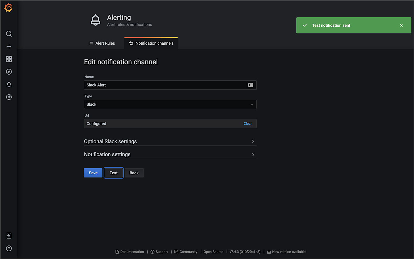
Below is an example of an alert based on an arbitrarily high CPU usage of 300 millicpu or millicores (m). When the CPU usage of a single pod goes above that value for more than 3 minutes, an alert is sent. The high CPU usage could be caused by the Horizontal Pod Autoscaler not functioning, or the HPA has reached its maxReplicas limit, or there are not enough resources available within the cluster’s existing worker nodes to schedule additional pods.

Triggered by the alert, Prometheus sends detailed notifications to the designated Slack channel.

Amazon CloudWatch Container Insights
Lastly, in the category of Metrics, Amazon CloudWatch Container Insights collects, aggregates, summarizes, and visualizes metrics and logs from your containerized applications and microservices. CloudWatch alarms can be set on metrics that Container Insights collects. Container Insights is available for Amazon Elastic Container Service (Amazon ECS), including Fargate, Amazon EKS, and Kubernetes platforms on Amazon EC2.

In Amazon EKS, Container Insights uses a containerized version of the CloudWatch agent to discover all running containers in a cluster. It then collects performance data at every layer of the performance stack. Container Insights collects data as performance log events using the embedded metric format. These performance log events are entries that use a structured JSON schema that enables high-cardinality data to be ingested and stored at scale.
In the previous post, we also installed CloudWatch Container Insights monitoring for Prometheus, which automates the discovery of Prometheus metrics from containerized systems and workloads.

Below is an example of a basic Performance Monitoring CloudWatch Container Insights Dashboard. The dashboard is filtered to the dev namespace of the EKS cluster, where the reference application platform is running. During this period, the backend services were put under a simulated load using hey. As the load on the application increased, the ‘Number of Pods’ increased from 20 pods to 56 pods based on the container’s requested resources and HPA configurations. There is also a CloudWatch Alarm, shown on the right of the screen. An alarm was triggered for an arbitrarily high level of network transmission activity.

Next is an example of Container Insights’ Container Map view in CPU mode. You see a visual representation of the dev namespace, with each of the backend service’s Service and Deployment resources shown.

Below, there is a warning icon indicating an Alarm on the cluster was triggered.

Lastly, CloudWatch Insights allows you to jump from the CloudWatch Insights to the CloudWatch Log Insights console. CloudWatch Insights will also write the CloudWatch Insights query for you. Below, we went from the Service D container metrics view in the CloudWatch Insights Performance Monitoring console directly to the CloudWatch Log Insights console with a query, ready to run.

Pillar 3: Traces
According to the Open Tracing website, distributed tracing, also called distributed request tracing, is used to profile and monitor applications, especially those built using a microservices architecture. Distributed tracing helps pinpoint where failures occur and what causes poor performance.
Header Propagation
According to Istio, header propagation may be accomplished through client libraries, such as Zipkin or Jaeger. Header propagation may also be accomplished manually, referred to as trace context propagation, documented in the Distributed Tracing Task. Alternately, Istio proxies can automatically send spans. Applications need to propagate the appropriate HTTP headers so that when the proxies send span information, the spans can be correlated correctly into a single trace. To accomplish this, an application needs to collect and propagate the following headers from the incoming request to any outgoing requests.
x-request-idx-b3-traceidx-b3-spanidx-b3-parentspanidx-b3-sampledx-b3-flagsx-ot-span-context
The x-b3 headers originated as part of the Zipkin project. The B3 portion of the header is named for the original name of Zipkin, BigBrotherBird. Passing these headers across service calls is known as B3 propagation. According to Zipkin, these attributes are propagated in-process and eventually downstream (often via HTTP headers) to ensure all activity originating from the same root are collected together.
To demonstrate distributed tracing with Jaeger and Zipkin, the gRPC Gateway passes the b3 headers. While the RESTful JSON-based services passed these headers in the HTTP request object, with gRPC, the heders are passed in the gRPC Context object. The following code has been added to the gRPC Gateway. The Istio sidecar proxy (Envoy) generates the initial headers, which are then propagated throughout the service call chain. It is critical only to propagate the headers present in the downstream request with values, as the code below does.
Below, in the CloudWatch logs, we see an example of the HTTP request headers recorded in a log message for Service A. The b3 headers are propagated from the gRPC Gateway reverse proxy to gRPC-based Go services. Header propagation ensures a complete distributed trace across the entire service call chain.

Headers propagated from Service A are shown below. Note the b3 headers propagated from the gRPC Gateway reverse proxy.
Jaeger
According to their website, Jaeger, inspired by Dapper and OpenZipkin, is a distributed tracing system released as open source by Uber Technologies. Jaeger is used for monitoring and troubleshooting microservices-based distributed systems, including distributed context propagation, distributed transaction monitoring, root cause analysis, service dependency analysis, and performance and latency optimization. The Jaeger website contains a helpful overview of Jaeger’s architecture and general tracing-related terminology.
If you deployed Jaeger using the Istio addons process demonstrated in part one of the previous post, access Jaeger similar to the other tools:
istioctl dashboard jaeger
Below are examples of the Jaeger UI’s Search view, displaying the results of a search for the Angular UI and the Istio Ingress Gateway services over a period of time. We see a timeline of traces across the top with a list of trace results below. As discussed on the Jaeger website, a trace is composed of spans. A span represents a logical unit of work in Jaeger that has an operation name. A trace is an execution path through the system and can be thought of as a directed acyclic graph (DAG) of spans. If you have worked with systems like Apache Spark, you are probably already familiar with the concept of DAGs.


Below is a detailed view of a single trace in Jaeger’s Trace Timeline mode. The 16 spans encompass nine of the reference platform’s components: seven backend services, gRPC Gateway, and Istio Ingress Gateway. The spans each have individual timings, with an overall trace time of 195.49 ms. The root span in the trace is the Istio Ingress Gateway. The Angular UI, loaded in the end user’s web browser, calls gRPC Gateway via the Istio Ingress Gateway. From there, we see the expected flow of our service-to-service IPC. Service A calls Services B and Service C. Service B calls Service E, which calls Service G and Service H.
In this demonstration, traces are not instrumented to span the RabbitMQ message queue nor MongoDB. You will not see a trace that includes a call from Service D to Service F via the RabbitMQ.

The visualization of the trace’s timeline demonstrates the synchronous nature of the reference platform’s service-to-service IPC instead of the asynchronous nature of the decoupled communications using the RabbitMQ messaging queue. Service A waits for each service in its call chain to respond before returning its response to the requester.
Within Jaeger’s Trace Timeline view, you have the ability to drill into a single span, which contains additional metadata. The span’s metadata includes the API endpoint URL being called, HTTP method, response status, and several other headers.

A Trace Statistics view is also available.

Additionally, Jaeger has an experimental Trace Graph mode that displays a graph view of the same trace.

Jaeger also includes a Compare Trace feature and two dependency views: Force-Directed Graph and DAG. I find both views rather primitive compared to Kiali. Lacking access to Kiali, the views are marginally useful as a dependency graph.

Zipkin
Zipkin is a distributed tracing system, which helps gather timing data needed to troubleshoot latency problems in service architectures. According to a 2012 post on Twitter’s Engineering Blog, Zipkin started as a project during Twitter’s first Hack Week. During that week, they implemented a basic version of the Google Dapper paper for Thrift.
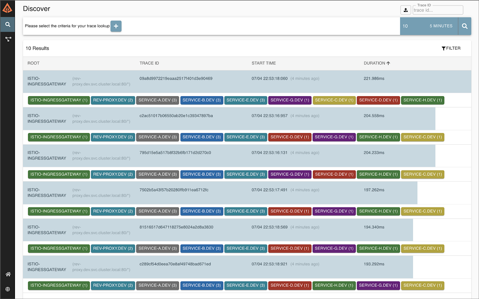
Zipkin and Jaeger are very similar in terms of capabilities. I have chosen to focus on Jaeger in this post as I prefer it over Zipkin. If you want to try Zipkin instead of Jaeger, you can use the following commands to remove Jaeger and install Zipkin from the Istio addons extras directory. In part one of the post, we did not install Zipkin by default when we deployed the Istio addons. Be aware that running both tools simultaneously in the same Kubernetes cluster will cause unpredictable tracing results.
kubectl delete -f https://raw.githubusercontent.com/istio/istio/release-1.10/samples/addons/jaeger.yaml
kubectl apply -f https://raw.githubusercontent.com/istio/istio/release-1.10/samples/addons/extras/zipkin.yaml
Access Zipkin similar to the other observability tools:
istioctl dashboard zipkin
Below is an example of a distributed trace visualized in Zipkin’s UI, containing 16 spans, similar to the trace visualized in Jaeger, shown above. The spans encompass eight of the reference platform’s components: seven of the eight backend services and the Istio Ingress Gateway. The spans each have individual timings, with an overall trace time of ~221 ms.

Zipkin can also visualize a dependency graph based on the distributed trace. Below is an example of a traffic simulation over a 24-hour period, showing network traffic flowing between the reference platform’s components, illustrated as a dependency graph.

Kiali: Microservice Observability
According to their website, Kiali is a management console for an Istio-based service mesh. It provides dashboards and observability, and lets you operate your mesh with robust configuration and validation capabilities. It shows the structure of a service mesh by inferring traffic topology and displaying the mesh’s health. Kiali provides detailed metrics, powerful validation, Grafana access, and strong integration for distributed tracing with Jaeger.
If you deployed Kaili using the Istio addons process demonstrated in part one of the previous post, access Kiali similar to the other tools:
istioctl dashboard kaili
For improved security, install the latest version of Kaili using the customizable install mentioned in Istio’s documentation. Using Kiali’s Install via Kiali Server Helm Chart option adds token-based authentication, similar to the Kubernetes Dashboard.

Kiali’s Overview tab provides a global view of all namespaces within the Istio service mesh and the number of applications within each namespace.

The Graph tab in the Kiali UI represents the components running in the Istio service mesh. Below, filtering on the cluster’s dev Namespace, we can observe that Kiali has mapped 11 applications (workloads), 11 services, and 24 edges (a graph term). Specifically, we see the Istio Ingres Proxy at the edge of the service mesh, gRPC Gateway, Angular UI, and eight backend services, all with their respective Envoy proxy sidecars that are taking traffic (Service F did not take any direct traffic from another service in this example), the external DocumentDB egress point, and the external Amazon MQ egress point. Note how service-to-service traffic flows with Istio, from the service to its sidecar proxy, to the other service’s sidecar proxy, and finally to the service.

Kiali allows you to zoom in and focus on a single component in the graph and its individual metrics.

Kiali can also display average request times and other metrics for each edge in the graph (communication between two components). Kaili can even show those metrics over a given period of time, using Kiali’s Replay feature, shown below.

The Applications tab lists all the applications, their namespace, and labels.

You can drill into an individual component on both the Applications and Workloads tabs and view additional details. Details include the overall health, Pods, and Istio Config status. Below is an overview of the Service A workload in the dev Namespace.

The Workloads detailed view also includes inbound and outbound network metrics. Below is an example of the outbound for Service A in the dev Namespace.

Kiali also gives you access to the individual pod’s container logs. Although log access is not as user-friendly as other log sources discussed previously, having logs available alongside metrics (integration with Grafana), traces (integration with Jaeger), and mesh visualization, all in Kiali, can act as a very effective single pane of glass for observability.

Kiali also has an Istio Config tab. The Istio Config tab displays a list of all of the available Istio configuration objects that exist in the user’s environment.

You can use Kiali to configure and manage the Istio service mesh and its installed resources. Using Kiali, you can actually modify the deployed resources, similar to using the kubectl edit command.

Oftentimes, I find Kiali to be my first stop when troubleshooting platform issues. Once I identify the specific components or communication paths having issues, I then review the specific application logs and Prometheus metrics through the Grafana dashboard.
Tear Down
To tear down the EKS cluster, DocumentDB cluster, and Amazon MQ broker, use the following commands:
# EKS cluster
eksctl delete cluster --name $CLUSTER_NAME
# Amazon MQ
aws mq list-brokers | jq -r '.BrokerSummaries[] | .BrokerId'aws mq delete-broker --broker-id {{ your_broker_id }}
# DocumentDB
aws docdb describe-db-clusters \
    | jq -r '.DBClusters[] | .DbClusterResourceId'aws docdb delete-
db-cluster \
    --db-cluster-identifier {{ your_cluster_id }}
Conclusion
In this post, we explored a set of popular open source observability tools, easily integrated with the Istio service mesh. These tools included Jaeger and Zipkin for distributed transaction monitoring, Prometheus for metrics collection and alerting, Grafana for metrics querying, visualization, and alerting, and Kiali for overall observability and management of Istio. We rounded out the toolset using Fluent Bit for log processing and forwarding to Amazon CloudWatch Container Insights. Using these tools, we successfully observed a gRPC-based, distributed reference application platform deployed to Amazon EKS.
This blog represents my own viewpoints and not of my employer, Amazon Web Services (AWS). All product names, logos, and brands are the property of their respective owners.
Continuous Integration and Deployment of Docker Images using GitHub Actions
Posted by Gary A. Stafford in Build Automation, Cloud, Continuous Delivery, DevOps, Go, Kubernetes, Software Development on June 16, 2021
According to GitHub, GitHub Actions allows you to automate, customize, and execute your software development workflows right in your repository. You can discover, create, and share actions to perform any job you would like, including continuous integration (CI) and continuous deployment (CD), and combine actions in a completely customized workflow.
This brief post will examine a simple use case for GitHub Actions — automatically building and pushing a new Docker image to Docker Hub. A GitHub Actions workflow will be triggered every time a new Git tag is pushed to the GitHub project repository.

GitHub Project Repository
For the demonstration, we will be using the public NLP Client microservice GitHub project repository. The NLP Client, written in Go, is part of five microservices that comprise the Natural Language Processing (NLP) API. I developed this API to demonstrate architectural principles and DevOps practices. The API’s microservices are designed to be run as a distributed system using container orchestration platforms such as Docker Swarm, Red Hat OpenShift, Amazon ECS, and Kubernetes.

Encrypted Secrets
To push new images to Docker Hub, the workflow must be logged in to your Docker Hub account. GitHub recommends storing your Docker Hub username and password as encrypted secrets, so they are not exposed in your workflow file. Encrypted secrets allow you to store sensitive information as encrypted environment variables in your organization, repository, or repository environment. The secrets that you create will be available to use in GitHub Actions workflows. To allow the workflow to log in to Docker Hub, I created two secrets, DOCKERHUB_USERNAME and DOCKERHUB_PASSWORD using my organization’s credentials, which I then reference in the workflow.

GitHub Actions Workflow
According to GitHub, a workflow is a configurable automated process made up of one or more jobs. You must create a YAML file to define your workflow configuration. GitHub contains many searchable code examples you can use to bootstrap your workflow development. For this demonstration, I started with the example shown in the GitHub Actions Guide, Publishing Docker images, and modified it to meet my needs. Workflow files are checked into the project’s repository within the .github/workflows directory.https://itnext.io/media/0e27d26012167bab83def6ef3595a74f
Workflow Development
Visual Studio Code (VS Code) is an excellent, full-featured, and free IDE for software development and writing Infrastructure as Code (IaC). VS Code has a large ecosystem of extensions, including extensions for GitHub Actions. Currently, I am using the GitHub Actions extension, cschleiden.vscode-github-actions, by Christopher Schleiden.

The extension features auto-complete, as shown below in the GitHub Actions workflow YAML file.

Git Tags
The demonstration’s workflow is designed to be triggered when a new Git tag is pushed to the NLP Client project repository. Using the workflow, you can perform normal pushes (git push) to the repository without triggering the workflow. For example, you would not typically want to trigger a new image build and push when updating the project’s README file. Thus, we use the new Git tag as the workflow trigger.


For consistency, I also designed the workflow to be triggered only when the format of the Git tag follows the common Semantic Versioning (SemVer) convention of version number MAJOR.MINOR.PATCH (v*.*.*).
on:
  push:
    tags:
      - 'v*.*.*'
Also, following common Docker conventions in the workflow, the Git tag (e.g., v1.2.3) is truncated to remove the letter ‘v’ and used as the tag for the Docker image (e.g., 1.2.3). In the workflow, theGITHUB_REF:11 portion of the command truncates the Git tag reference of refs/tags/v1.2.3 to just 1.2.3.
run: echo "RELEASE_VERSION=${GITHUB_REF:11}" >> $GITHUB_ENV
Workflow Run
Pushing the Git tag triggers the workflow to run automatically, as seen in the Actions tab.


Detailed logs show you how each step in the workflow was processed.
The example below shows that the workflow has successfully built and pushed a new Docker image to Docker Hub for the NLP Client microservice.

Failure Notifications
You can choose to receive a notification when a workflow fails. GitHub Actions notifications are a configurable option found in the GitHub account owner’s Settings tab.

Status Badge
You can display a status badge in your repository to indicate the status of your workflows. The badge can be added as Markdown to your README file.

Docker Hub
As a result of the successful completion of the workflow, we now have a new image tagged as 1.2.3 in the NLP Client Docker Hub repository: garystafford/nlp-client.

Conclusion
In this brief post, we saw a simple example of how GitHub Actions allows you to automate, customize, and execute your software development workflows right in your GitHub repository. We can easily extend this post’s GitHub Actions example to include updating the service’s Kubernetes Deployment resource file to the latest image tag in Docker Hub. Further, we can trigger a GitOps workflow with tools such as Weaveworks’ Flux or Argo CD to deploy the revised workload to a Kubernetes cluster.

This blog represents my own viewpoints and not of my employer, Amazon Web Services (AWS). All product names, logos, and brands are the property of their respective owners.
-
You are currently browsing the archives for the Build Automation category.
Gary Stafford
AWS Area Principal Solutions Architect | 10x AWS Certified Pro | DevOps | Data/ML | Serverless | Polyglot Developer | Former ThoughtWorks and Accenture
